A decision between Bayesian and Frequentist upper limit in analyzing continuous Gravitational Waves

Abstract

Given the sensitivity of current ground-based Gravitational Wave (GW) detectors, any continuous-wave signal we can realistically expect will be at a level or below the background noise. Hence, any data analysis of detector data will need to rely on statistical techniques to separate the signal from the noise. While with the current sensitivity of our detectors we do not expect to detect any true GW signals in our data, we can still set upper limits (UL) on their amplitude. These upper limits, in fact, tell us how weak a signal strength we would detect. In setting upper limit using two popular method, Bayesian and Frequentist, there is always the question of a realistic results. In this paper, we try to give an estimate of how realistically we can set the upper limit using the above mentioned methods. And if any, which one is preferred for our future data analysis work.

I Introduction

Gravitational Waves (GWs), ripples in space-time which travel at the speed of light, are a fundamental consequence of Einstein’s General Theory of Relativity. Due to the great distance to any likely detectable sources of GWs, the signal amplitude reaching us will be very small. Because of limitations in technology, there have been no direct detections of GWs so far. However, with the future generation of detectors, like Advanced LIGO, we should be able to detect a variety of sources.

Because of their nature, continuous GWs (emitting from axisymetric rotating neutron stars) reaching Earth are expected to be extremely weak. Therefore even with the quite significant sensitivity of our current detectors, it will be difficult to detect them. One possible way to increase the overall signal compared to the background noise (signal-to-noise ratio (SNR)) is to coherently integrate the data for several days up to few years.

The basic problem in GW detection is to identify a gravitational waveform in a noisy background. Because all data streams contain random noise, the data are just a series of random values and therefore the detection of a signal is always a decision based on probabilities. The aim of detection theory is therefore to assess this probability.

The basic idea behind the current methods of signal detection is that the presence of a signal will change the statistical characterization of the data $x(t)$, in particular its probability distribution function (pdf) $P(x)$. Recall that the pdf is defined so that the probability of a random variable $x_{i}$ lies in an interval between $x(t)$ and $x(t)+dx$ is $P(x)dx$. Let us denote by $P(x|0)$ the probability of a random process $x(t)$ (representing our data) in the absence of any signal, and by $P(x|h)$ the probability of that same process when a signal $h(t)$ is present. Given a particular measurement $x(t)$ obtained with our detector, is its probability distribution given by $P(x|0)$ or $P(x|h)$? In order to make that decision, we need to make a rule called a statistical test.

There are several approaches to find an appropriate test, notably the Bayesian, Minimax and Neyman-Pearson approach (for an overview, we refer the reader to Jaranowski and  Królak, LRR-JK and the references listed therein). In the end, however, these three approaches lead to the same test, namely the likelihood ratio test LRR-JK ; davis .

Among the three main approaches, the Neyman-Pearson approach is often used in the detection of gravitational waves schutz-gr-qc-9710080 . This approach is based on maximizing the detection probability (equivalently minimizing the false dismissal rate) for fixed false alarm rate, where the detection probability is the probability that the random value of a process which contains the signal will pass our test, while the false alarm probability is the probability that data containing no signal will pass the test nonetheless. Mathematically, we can express the Detection and False Alarm probabilities as schutz-gr-qc-9710080

$$P_{D}(R) = \int_{R}P(x|h)dx,$$ (1)

$$P_{F}(R) = \int_{R}P(x|0)dx,$$ (2)

respectively, where $R$ is the detection region (to be determined).

The Likelihood ratio $\Lambda$ is the ratio of the pdf when the signal is present to the pdf when it is absent:

$$\Lambda={P(x(t)|h(t))\over P(x(t)|0)}.$$ (3)

Taking the data to be $x(t)=h(t)+n(t)$, with $h(t)$ the signal and $n(t)$ the noise and with the assumption that the noise is a zero-mean, stationary and Gaussian random process, we can write the likelihood ratio as

$$\Lambda = {P(x|h)\over P(x|0)}$$ (4)

$$= {\exp(-{1\over 2}(x-h|x-h))\over\exp(-{1\over 2}(x|x))}$$

$$= \exp[(x|h)-{1\over 2}(h|h)].$$

This leads to the log of likelihood function as

$$\log\Lambda=(x|h)-{1\over 2}(h|h).$$ (5)

We can also rewrite the simple expression of Eq. (5) for the likelihood function in terms of the new variables, $A^{a}$ and $h_{a}$, as

$$\log\Lambda=(x|A^{a}h_{a})-{1\over 2}(A^{a}h_{a}|A^{b}h_{b}).$$ (6)

where the constant (in time) amplitudes $A^{a}=A^{a}(h_{0},\psi,i,\Phi_{0})$ are CS

$$A^{1} = ~{}~{}A_{+}\cos{\Phi_{0}}\cos{2\psi}-A_{\times}\sin{\Phi_{0}}\sin{2\psi},$$ (7)

$$A^{2} = ~{}~{}A_{+}\cos{\Phi_{0}}\sin{2\psi}+A_{\times}\sin{\Phi_{0}}\cos{2\psi},$$ (8)

$$A^{3} = -A_{+}\sin{\Phi_{0}}\cos{2\psi}-A_{\times}\cos{\Phi_{0}}\sin{2\psi},$$ (9)

$$A^{4} = -A_{+}\sin{\Phi_{0}}\sin{2\psi}+A_{\times}\cos{\Phi_{0}}\cos{2\psi}.$$ (10)

and

$$h_{1}(t) = a(t)\cos\phi(t),$$ (11)

$$h_{2}(t) = b(t)\cos\phi(t),$$ (12)

$$h_{3}(t) = a(t)\sin\phi(t),$$ (13)

$$h_{4}(t) = b(t)\sin\phi(t),$$ (14)

where $a(t)$ and $b(t)$ are functions of right ascension $\alpha$ and declination $\delta$; they are independent of $\psi$, and $\phi$ is the phase of the wave signal seen at the Solar System Barycenter (SSB) jks . Likewise

$$A_{+} = {1\over 2}h_{0}(1+\cos^{2}{\iota}),$$ (15)

$$A_{\times} = h_{0}\cos{\iota},$$ (16)

where $h_{0}$ is the wave amplitude, $\iota$ the inclination angle, $\psi$ the polarization angle and $\Phi_{0}$ the initial phase.

Since the $A^{a}$s depend neither on the detector properties nor on the frequency or the time, we can take them out of the inner product and write the log of likelihood ratio as

$$\log\Lambda=A^{a}(x|h_{a})-{1\over 2}A^{a}A^{b}(h_{a}|h_{b}).$$ (17)

Defining the new variables

$$H_{a}\equiv(x|h_{a}),$$ (18)

and

$$M_{ab}\equiv(h_{a}|h_{b}),$$ (19)

we have

$$\log\Lambda=A^{a}H_{a}-{1\over 2}A^{a}A^{b}M_{ab}.$$ (20)

The maximum detection probability follows from the maximization of the likelihood function: by maximizing the likelihood function with respect to the $A^{a}$ (which, again, are independent of the detector), we have

$${\partial\log\Lambda\over\partial A^{a}}=0.$$ (21)

This leads us to

$$H_{a}-A^{b}_{\text{\tiny MLE}}M_{ab}=0,$$ (22)

and therefore

$$A^{b}_{\text{\tiny MLE}}=(M^{-1})^{ab}H_{a}.$$ (23)

The label MLE denotes the Maximum Likelihood Estimator; it corresponds to the values for the $A^{a}$s we calculate from our data by maximizing the likelihood ratio (so that, in practice, we are calculating $A^{a}=E[A^{a}_{\tiny MLE}]$). By definition, the $\mathcal{F}$-Statistic is the maximum of the logarithm of likelihood function. Substituting Eq. (23) into Eq. (20), we have

$$\mathcal{F}\equiv\log\Lambda\mid_{\text{\tiny MLE}}={1\over 2}~{}H_{a}~{}(M^{-1})^{ab}~{}H_{b}.$$ (24)

This is the $\mathcal{F}$-Statistic which a generalized version of that for the multi-IFO (Interferometer Observatory) can be found in iraj-thesis .

Again by writing the data as $x(t)=n(t)+h(t)$, and using Eq. (2.5) of Cutler-Schutz (CS) CS indicating that $\langle(x|n)(y|n)\rangle=(x|y)$ with this fact that $\langle(h|n)\rangle=0$, we would have the following

$$\langle 2\mathcal{F}\rangle=4+(h|h),$$ (25)

which follows a $\chi^{2}$ distribution with 4 degrees of freedom and non-centrality parameter $\rho^{2}\equiv(h|h)$, that is the square of optimal signal to noise ratio (SNR²). The degrees of freedom come from the 4 unknown parameters of pulsar namely the amplitude ($h_{0}$), inclination angle ($\iota$), polarization angle ($\psi$) and the initial phase ($\Phi_{0}$). As was described in CS , even for a multi-IFO the number of freedom will remain unchanged, since we always have the same 4 unknown parameters in entire the search.

The $\mathcal{F}$-statistic shown above, which was originally derived by Jaranowski, Królak and Schutz (JKS)jks , is the optimal statistic for detection of nearly periodic gravitational waves from GW pulsars. We can use this statistical tool to search for any kind of pulsars; unknown sources or targeted search. In targeted search we know everything about the source by using some other astronomical techniques, such as radio astronomy, gamma and X-ray astronomy etc. The main information required for our search are; frequency and its derivatives and position of the source. Given all these information to the software developed by the LSC (LIGO Scientific Collaboration) lal ; lal-doxygen (the implementation to our work can be found in iraj-thesis ), and using a single workstation, we will be able to search a known pulsar in a few minutes.

The work in this paper was done using simulated data for 100 arbitrary pulsars. To set the positions and the frequencies of these simulated pulsars, we have used the data of the known pulsars, as given in the Australian Telescope National Facilities (ATNF) catalogue ATNF . To make the simulated data more realistic, we generated the data at the level of LIGO detectors sensitivity. Since our detectors (initial LIGO and even Enhanced LIGO) are not sensitive enough to detect any signal until now, we assume that the data are just simply noise without any signal in them. Due to that, our simulated data are just pure noise and therefore instead of looking for any detection, we set the upper limit on the strength of the gravitational wave signal. For the historical reason we take the value of 95$\%$ for the upper limit. All the search done in this paper are in frequency domain. As the main goal of this paper is to compare two different approaches in setting upper limits, we use Bayesian and Frequentist algorithm to perform it on the same data for each pulsar. These two algorithms will be explained in more details below.

II Frequentist Upper Limits

The frequentist probability of an event represents the expected frequency of occurrence of that event. The result for our upper limits depends crucially on the experimental data under examination. The confidence value associated with these upper limits indicates the expected occurrence of detection statistics values more significant than the one that we have measured in the presence of signals whose amplitude is equal to the upper limit value.

To set the frequentist upper limit on the amplitude of gravitational waves, we use the $\mathcal{F}$-statistic as an optimal detection statistic. To start with, we need to assign a confidence level $\mathcal{C}$ – roughly speaking, our criterion will then be that, for our “repeated measurements”, in $\mathcal{C}$-percent of the time the value of $2\mathcal{F}$ is above a specified threshold.

Let us explain how this works in detail for the example of setting a 95% upper limit on $h_{0}$. For this, we need to find at which $h_{0}$ it is true that 95% of the values of the $\mathcal{F}$-statistic are above the initial value of $2\mathcal{F}$ derived from the data. To do so, we proceed step by step as follows:

1. Compute the $\mathcal{F}$-statistic of a perfectly matched signal using the exact values for the signal parameters (such as frequency, longitude, latitude and frequency derivatives). Let us call the resulting value of the $\mathcal{F}$-statistic $\mathcal{F}^{*}$.

2. Estimate the signal amplitude, $h_{0}$, using our parameter estimation routine.

3. Take this $h_{0}$ as the initial value of the search.

4. Since we assume that there is no signal in the data – that it is pure noise –, we can randomly assign arbitrary values to the other signal parameters (such as $\phi_{0}$, $\psi$ and $\cos{\iota}$).

5. To determine the probability distribution of $\mathcal{F}$-statistic, we take a random frequency value with a band of $0.1$Hz around the actual pulsar frequency (as was proposed in the LIGO S1 paper S1:pulsar ) and inject the artificial signal. With this choice, we are sure to be on the safe side; we use a large amount of data (in order of several months up to a year), so that the $0.1$Hz band will not lead to any spurious correlations between the search parameters.

6. After injection, compute the $\mathcal{F}$-statistic once again. Let us designate the resulting value of $2\mathcal{F}$ as $\mathcal{F}^{\prime}$; store this value for later use.

7. Repeat the injections, computing of $\mathcal{F}$-statistic for 150 times. Save all resulting values of $\mathcal{F}^{\prime}$. (The number of iterations used here is a heuristic value.)

8. As we are looking for a 95% upper limit, proceed as follows: if the confidence level (the percentage of instances in which $\mathcal{F}^{\prime}$ is greater than $\mathcal{F}^{*}$) was less than $90\%$ or above $98\%$ (say $x$), multiply the $h_{0}$ by the ratio of ${95\over x}$ and take this value as the initial $h_{0}$ for the next step.

9. Repeat steps “6” and “7” until the confidence level is in one of the following ranges: a) $90\%-95\%$, or b) $95\%-98\%$.

10. For case a), multiply $h_{0}$ by 1.05; for case b), multiply by 0.90. (The factors 1.05 and 0.90 are, again, heuristic.)

11. Repeat the calculations of step “7” and following, but this time with 1000 injections in each run (instead of 150) to improve the statistics.

12. Repeat step “11” for 6 times; in each run follow the instructions in step “10”. (The number of repetitions is heuristic; it is chosen in a way that the range of computed confidence levels will always include values higher and lower then 95%; therefore we can make an ”interpolation” fit instead of having to extrapolate.)

A flow chart version of this procedure can be found in Fig. 1.

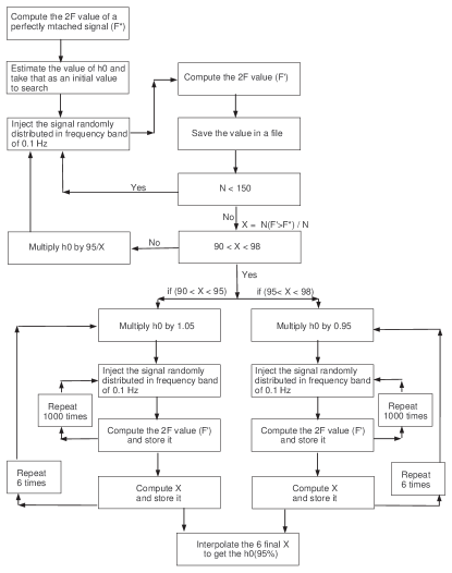
Figure 1: A Flow-Chart of how we implemented the frequentist upper limit.

III Bayesian Upper Limit

The Bayesian probability is a measure of degree of belief in the occurrence of a statistical process. In contrast with the Frequentist probability, in the Bayesian approach, we do not need for an event of that particular type to have actually happened; all we need is to find a measure for the degree to which a person believes that a given proposition is true.

III.1 Theoretical approaches

The key ingredient of the Bayesian approach is the Bayes’ theorem (a simple proof of that can be found in cowan )

$$P(A|B)={P(B|A)P(A)\over P(B)}.$$ (26)

The term at the left hand side is called the posterior probability, while $P(A)$ is the prior probability which reflects our initial knowledge about the quantity $A$. The term $P(B|A)$ is called the likelihood function; the log of this is, in fact, the $\mathcal{F}$-statistic to be computed from our data.

Our goal is to set an upper limit on the strength of the gravitational wave amplitude, $h_{0}$, using a given amount of available data – which is the posterior probability of $h_{0}$ that we look for. Therefore, our data plays the role of $B$ in Eq. (26); which we denote it by $s$. The term $A$ is the quantity about which we intend to draw conclusions using our data; in our case, this is the upper limit $h_{0}$, so we will substitute $h_{0}$ for $A$ in what follows. With these substitutions, Eq. (26) now reads

$$P(h_{0}|s)={P(s|h_{0})\times P(h_{0})\over P(s)},$$ (27)

where $P(h_{0}|s)$ is the conditional probability of $h_{0}$ (posterior probability) given the data $s$, $P(s|h_{0})$ is the likelihood function (to be defined below), and $P(h_{0})$ represents our prior knowledge about the distribution of $h_{0}$.

Since the term $P(s)$ is independent of our signal, we can consider it as the constant normalization factor; it will cancel out automatically when we compute the confidence level. Therefore, we can rewrite our Bayes’ theorem for the general case of all signal parameters as

$$P(h_{0},\psi,\iota,\Phi_{0}|s)\propto P(s|h_{0},\psi,\iota,\Phi_{0})\times P(h_{0},\psi,\iota,\Phi_{0}),$$ (28)

where, again, $P(h_{0},\psi,\iota,\Phi_{0}|s)$ is our posterior probability (to be calculated), $P(s|h_{0},\psi,\iota,\Phi_{0})$ is the likelihood function and $P(h_{0},\psi,\iota,\Phi_{0})$ is the prior probability of $h_{0},\psi,\iota,\Phi_{0}$.

There are two common choices for estimating prior probability, known as a flat prior and Jeffrey’s prior. In the flat prior, the prior probability is chosen to be constant ($P(h_{0})\equiv constant$), while in Jeffrey’s prior, it is taken to vary inversely proportional to the value of $h_{0}$ ($P(h_{0})\equiv 1/h_{0}$). For more details we refer the reader to gregory and a comparison for this case can be found in rejean-thesis .

The Jeffrey’s prior gives a higher value in upper limit than the flat prior, while a flat prior gives a more realistic value for our case rejean-thesis . Therefore in the following we will focus on a flat prior, as the case followed in iraj-thesis .

To obtain the posterior probability, we need to calculate the likelihood function. By Eq. (24), it can be expressed as

$$P(s|h_{0},\psi,\iota,\Phi_{0})\propto\text{e}^{-{1\over 2}M_{ab}(A^{a}-A^{a_{0}})(A^{b}-A^{b_{0}})}=G,$$ (29)

where $A=(A^{1},~{}A^{2},~{}A^{3},~{}A^{4})(h_{0},\psi,\iota,\Phi_{0})$ are the four amplitude parameters defined in Eqs. (7-10) and $G=G(h_{0},\psi,\iota,\Phi_{0})$. The $A^{0}=(A^{1_{0}},~{}A^{2_{0}},~{}A^{3_{0}},~{}A^{4_{0}})$ are also the best fit for the $A^{a}$s resulting from our calculation of the $\mathcal{F}$-statistic.

For proper normalization, we first compute the integral

$$I\equiv\int_{0}^{\infty}P(h_{0})dh_{0}\int_{-1}^{1}d\mu\int_{-\pi/4}^{\pi/4}d\psi\int_{0}^{2\pi}d\Phi_{0}~{}G,$$ (30)

where $\mu\equiv\cos{\iota}$, and we will set ‘$P(h_{0})\equiv constant$’. To find the upper limit we use $h_{0}^{max}$ as the upper bound in the integration over $h_{0}$,

$$I_{UL}\equiv\int_{0}^{h_{0}^{max}}P(h_{0})dh_{0}\int_{-1}^{1}d\mu\int_{-\pi/4}^{\pi/4}d\psi\int_{0}^{2\pi}d\Phi_{0}~{}G.$$ (31)

We select $h_{0}^{max}$ in such a way that the ratio $I_{UL}/I$ gives us the desired confidence level. In our case, we are looking for the $95\%$ upper limit, therefore

$${I_{UL}\over I}=0.95.$$ (32)

III.2 Practical implementation

To implement the above formalism, let us first construct the function $G(h_{0},\psi,\iota,\Phi_{0})$. To do so, we need to expand the matrix of Eq. (19). The elements of this matrix depend on the three amplitude modulation coefficients ($A,~{}B$ and $C$) defined in CS . Based on the notation used here, these elements take the form of

$$M_{ab}=\left[\begin{array}[]{cccc}A/2&C/2&0&0\\ C/2&B/2&0&0\\ 0&0&A/2&C/2\\ 0&0&C/2&B/2\end{array}\right],$$ (33)

which a detailed procedure of their derivation can be found iraj-thesis . Then we can construct the four elements

$$G_{1} = {A\over 2}(A^{1}-A^{1_{0}})^{2}+{C\over 2}(A^{1}-A^{1_{0}})(A^{2}-A^{2_{0}}),$$ (34)

$$G_{2} = {B\over 2}(A^{2}-A^{2_{0}})^{2}+{C\over 2}(A^{2}-A^{2_{0}})(A^{1}-A^{1_{0}}),$$ (35)

$$G_{3} = {A\over 2}(A^{3}-A^{3_{0}})^{2}+{C\over 2}(A^{3}-A^{3_{0}})(A^{4}-A^{4_{0}}),$$ (36)

$$G_{4} = {B\over 2}(A^{4}-A^{4_{0}})^{2}+{C\over 2}(A^{4}-A^{4_{0}})(A^{3}-A^{3_{0}}),$$ (37)

to make the final form of $G(h_{0},\psi,\iota,\Phi_{0})$ in Eqs. (30) and (31) as

$$G=\exp[-{1\over 2}(G_{1}+G_{2}+G_{3}+G_{4})].$$ (38)

This is the core equation for our upper-limit analysis in Bayesian approach. To construct this, we need all the above mentioned parameters to be resulted from our software. The software we have used for this purpose was developed partly by the author of this paper and is now part of the LAL (LIGO Algorithm Library) lal . With this software we calculate the four amplitudes $A^{a}$ as well as the matrix elements $M_{ab}$ (namely the amplitude modulation coefficients $A,B$ and $C$). Once we have constructed the likelihood function $G(h_{0},\psi,\iota,\Phi_{0})$, we can calculate the UL value in Eq. (32) in two ways. One is to follow the exact procedure spelled out above; first calculating the normalization in Eq. (30) and then trying to find a value of $h_{0}^{max}$ for which the ratio of Eq. (32) will be satisfied. This can be done using the Numerical Integration routines in mathematical software like Mathematica and Maple. Another way would be to calculate the posterior probability of $h_{0}$ by marginalizing over the other three parameters. This can be expressed in mathematical form as

$$p(h_{0}|s)\propto\int\int\int G(h_{0},\psi,\iota,\Phi_{0})~{}d\psi~{}d\mu~{}d\Phi_{0}.$$ (39)

Once the posterior probability for $h_{0}$ is known, one can then integrate it over a sufficient range of $h_{0}$ to find out the area covered; the result can be used for proper normalization (namely unit total area). Next, we can find out at which $h_{0}$ the fraction of area would satisfy our required confidence level.

Both the above methods have given equivalent results as discussed in details in iraj-thesis . However, for the work expressed in this paper, we followed the second algorithm.

IV Results and discussion

Once again, we have selected 100 arbitrary pulsars frequencies and positions (based on the real pulsars information taken from ATNF ATNF ). We have generated the simulated data at the level of current LIGO detectors sensitivity (using the LAL software lal ; lal-doxygen developed by LSC) and computed the UL for these pulsars. To compare with the real data, the simulated data contains just noises where the upper limit set on them are shown in Fig. 2.

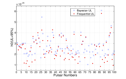
Figure 2: The upper limits value on the $h_{0}$ for 100 arbitrary pulsars using simulated data. In this plot, both Bayesian and Frequentist ULs are shown.

The blue rectangular in this plot represent the value of upper limits in Bayesian approach and the red circle points to the Frequentist ones. The horizontal axis indicates the pulsars number, therefore on each vertical line corresponds to each pulsar we should have one blue rectangular and one red circle. However, as seen, in some cases there is just one blue rectangular and missing red circle (Frequentist UL). These count for 16 pulsars, in which 7 of them were caused due to some unknown reason. The reason for the 9 others is that; in these cases, due to very small amount of $2\mathcal{F}$, the Frequentist upper limit procedure could not be converged to any particular value. It means, for some cases, by changing (increasing or decreasing) the value of $h_{0}$ for more than two order of magnitude, the upper limit value always stands above 96% or 97%.

An example of that is shown in Fig. 3, that is the case where $2\mathcal{F}=0.08$. This figure shows the dependency of Frequentist upper limit to $h_{0}$ for an individual pulsar. It’s clear that even by increasing the $h_{0}$ for about $2.5$ order of magnitude, the value of upper limit lies mostly about 100%. While, in general the upper limit is very sensitive to small changes in $h_{0}$. This was done 76 times and in each time the value of $h_{0}$ was increased according to the procedure expressed in Sec. II. Note that the starting and ending value of $h_{0}$ are significantly smaller than the $h_{0}$ require for $95\%$ upper limit shown in Fig. 2. Means that, in normal condition where the required $h_{0}$ to get $95\%$ upper limit is in order of $10^{-26}$, by setting the $h_{0}$ in the range of $10^{-28}-10^{-27}$, we should get a very small upper limit compare to $95\%$. In fact, as disscused below, the low value of $2\mathcal{F}$ for this pulsar is the reason of such a behavior in the Frequentist framework.

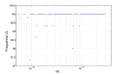
Figure 3: One of the bad upper limit value on the $h_{0}$ in Frequentist approach. The value of $2\mathcal{F}$ for this case was $0.08$.

The same behavior was shown in iraj-thesis ; iraj-defense by using the real data. The reason is clear; we have pointed out that the Frequentist approach is based on the number of occurance of an event. For this we should set a threshold and count how many times the value of that particular parameter is passing this threshold. Naturally there can be some False Alarms (FA), which a noise shows itself strong enough to pass this threshold. Since the $\mathcal{F}$-statistic follows a $\chi^{2}$ distribution with four degrees of freedom, the FA follows as (equation 3.44 of iraj-thesis ),

$$\alpha=(1+2\mathcal{F})~{}\mbox{e}^{-2\mathcal{F}}.$$ (40)

The values of $2\mathcal{F}$ in which the Frequentist upper limit could not be converged are: $0.08,0.34$, $0.46,0.47$, $0.49,0.51$, $0.59,0.63$ and $0.84$. So, by putting these numbers in the above equation we get a very large values of FA. For example, in the case of $2\mathcal{F}=0.84$ we have $\alpha=0.80$, $2\mathcal{F}=0.46$ gives $\alpha=0.92$ and for $2\mathcal{F}=0.08$ we get $\alpha=0.997\sim 100$. This explains the whole story.

This high false alarm probability means that noise alone has a high chance of producing an $\mathcal{F}$-statistic value greater than the $\mathcal{F}^{*}$ produced by our data set and our template. In other words, our realization of the noise is one that; it is particularly unlikely to look like it contains our signal, and this statistical fluctuation yields a low upper limit value or even does not converge – due to the nature of the procedure that we use to determine the upper limit. The Bayesian approach is less sensitive to such fluctuations. Note that the resulting frequentist upper limit is not an artifact of our technique, but it is still a perfectly correct and consistent upper limit in the Frequentist framework. This clearly shows the nature of our data.

To investigate further and check the behavior of the Frequentist UL, let us compare its value with that of Bayesian. To do so, we plot the ratio of the Bayesian UL over the corresponding value of Frequentist for the same pulsar versus the value of $2\mathcal{F}$ (Fig. 4). The output says; as we go further to the value of $2\mathcal{F}$ less than $4$, the ratio increases and when we reach to the $2\mathcal{F}=1$, this ratio is quite significant; about a factor of $2.3$. For the case of $2\mathcal{F}<1$, we have already seen that the upper limit for the Frequentist approach did not converge. Therefore they are not shown in this plot. If they would converge, they should be quite lower than that of Bayesian and therefore the ratio should go much higher. The same behavior was shown in iraj-thesis with real data.

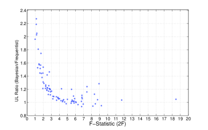
Figure 4: The ratio of Bayesian over Frequentist upper limits value on the $h_{0}$ for 100 arbitrary pulsars using simulated data.

Fig. 4 also shows that, at roughly $2\mathcal{F}=4$ the ratio is close to unity and roughly remains the same when $2\mathcal{F}>4$. This tells that the problem of low value in upper limit in Frequentist approach appears when we have $2\mathcal{F}<4$ while for larger value of $\mathcal{F}$-statistic there is always agreement between Frequentist and Bayesian frameworks.

Apart from the difference in the nature of Frequentist and Bayesian frameworks, there is another difference in performing a Frequentist and the Bayesian upper limit search. Since in Frequentist algorithm we need to inject some artificial signals into the data and then search the newly generated data to compute the $\mathcal{F}$-statistic in each iteration, this requires a high amount of computational resources. To increase the sensitivity we need to use more data that requires more computational power as well. Because, the required time to search the data to compute the $\mathcal{F}$-statistic is linearly proportional to the amount of data. In order to have a better statistic in Frequentist algorithm, we therefore need a larger iteration. This would additionally brings another linear increment in the cost for the computation. While in the Bayesian approach, to compute the $\mathcal{F}$-statistic and the other components, we search the data just once. Then compute the $P(h_{0})$ by marginalizing the probability over the $\psi,\iota$ and $\Phi_{0}$. These all will be done once and are computationally very cheap. As an estimation, the entire process for one pulsar using Bayesian algorithm takes about half an hour up to one hour in a single workstation. In a good approximation this is independent of the amount of data. Because, searching in the large amount of data (say about one year) to compute the $\mathcal{F}$-statistic and other components takes just about few minutes. In contrary, the required time for a Frequentist algorithm to search for single pulsar in an amount of data in order of one year takes about 3 weeks on a single workstation.

As a summary; although search in the Frequentist upper limit shows the exact nature of our data, however there are some disadvantages with the same search by using the Bayesian algorithm. The important one is that in the case where our data shows a small value of $\mathcal{F}$-statistic in a particular frequency bin and position of the pulsar, we cannot trust the upper limit value produced by Frequentist approach. Likewise, performing a search in the Frequentist framework is much expensive than the same search in Bayesian approach.

V Distribution of 95% Bayesian upper limits on $h_{0}$ using simulated data in frequency domain

As an application of Bayesian algorithm, we now present the distribution of ULs (95% upper limit on $h_{0}$) computed in the Frequency Domain (FD). We start with the idealized case of a large number (5500) of simulated data set with pure noises (no signal), and compute the 95% upper limit on $h_{0}$ of each data set. The sky locations in the search are chosen randomly such that their distribution over the solid angle is uniform; detectors position are picked randomly from a list consisting of the locations of H1, L1, VIRGO and GEO600 detectors. The resulting mean upper limit is

$$\langle h_{0}^{95\%}\rangle=(10.67\pm 0.04)\sqrt{S_{h}(f)\over T}.$$ (41)

In order to compare our result with the simulation in Time Domain (TD) done by Dupuis and Woan rejean-graham , we repeated this experiment with only H1, L1 and GEO600 detectors, as in their analysis. The results are in a very good agreement with a ratio in ULs

$${\langle h_{0}^{95\%}\rangle_{FD}\over\langle h_{0}^{95\%}\rangle_{TD}}=0.98.$$ (42)

Fig. 5 shows the distribution of $h_{0}^{95\%}$ for 5500 different runs in frequency domain, which is also in a good agreement with that of presented in rejean-graham .

These results show that although we use different domain (TD or FD) to search for gravitational waves, if we stay in Bayesian framework, both give the same results theoretically (a more details can be found in iraj-thesis ). However, using different frameworks (Frequentist or Bayesian) will may lead to a different outcome.

Figure 5: Distribution of 95% Bayesian upper limit on $h_{0}$ using 5500 individual simulated data runs in frequency domain. $\langle h_{0}^{95\%}\rangle=(10.59\pm 0.04)$.

References

- (1) P. Jaranowski, A. Królak, Living Rev. Relativity 8,(2005), 3.
- (2) M.H.A. Davis, “A review of Statistical Theory of Signal Detection”, in B.F. Schutz, ed., Gravitational Wave Data Analysis, Proceeding of the NATO Advanced Research Workshop, held at Dyffryn House, St. Nicholas, Cardiff, Wales, 6-9 July 1987, vol. 253 of NATO ASI Series C, 73-94.
- (3) Bernard, F. Schutz, Introduction to the Analysis of Low-Frequency Gravitational Wave Data, gr-qc/9710080.
- (4) Curt Cutler and Bernard F. Schutz, Phys. Rev. D72, 063006 (2005).
- (5) P. Jaranowski, A. Królak, and B.F. Schutz (JKS), Phys. Rev. D58, 063001 (1998).
-
(6)
The LAL software can be found on the following websites:
http://www.lsc-group.phys.uwm.edu/daswg/
projects/lalapps.html -
(7)
The doxygen version of the LAL softwares can be
found in this
site:
http://www.lsc-group.phys.uwm.edu/lal/
slug/nightly/doxygen/html/dirs.html - (8) Iraj Gholami, PhD thesis, Potsdam University, Germany (2008), http://opus.kobv.de/ubp/volltexte/2008/1880/.
-
(9)
The Australian Telescope National Facility
catalogue
http://www.atnf.csiro.au/research/pulsar/psrcat/ - (10) B. Abbott et al.. (The LIGO Scientific Collaboration), Phys. Rev. D69, 082004 (2004).
- (11) Glen Cowan, Statistical Data Analysis, Oxford Science Publications, 1998.
- (12) P.C. Gregory, Bayesian Logical Data Analysis for the Physical Sciences, Cambridge University Press, 2005.
- (13) Réjean Dupuis, PhD Thesis, University of Glasgow (2004).
- (14) Iraj Gholami, PhD thesis defense presentation, 2008.
- (15) Réjean Dupuis and Graham Woan, Bayesian estimation of pulsar parameters from gravitational wave data, Phys. Rev. D72, 102002 (2005).