Holographic dark matter and dark energy with second order invariants
Abstract
One of the main goals of modern cosmology remains to summon up a self consistent policy, able to explain, in the framework of the Einstein’s theory, the cosmic speed up and the presence of Dark Matter in the Universe. Accordingly to the Holographic principle, which postulates the existence of a minimal size of a physical region, we argue, in this paper, that if this size exists for the Universe and it is accrued from the independent geometrical second order invariants, it would be possible to ensure a surprising source for Dark Matter and a viable candidate for explaining the late acceleration of the Universe. Along the work, we develop low redshift tests, such as Supernovae Ia and kinematical analysis complied by the use of Cosmography and we compare the outcomes with higher redshift tests, such as CMB peak and anisotropy of the cosmic power spectrum. All the results indicate that the models presented here can be interpreted as unified models that are capable to describe both the dark matter and the dark energy.
pacs:
98.80.-k, 98.80.Jk, 98.80.EsI Introduction
General Relativity has been deemed as one of the cornerstones of modern theoretical physics. All its predictions, especially in the Solar System regime, found numerous experimental evidences cliff . Despite the theory promises to completely clear up the dynamical properties of the whole Universe, many attempts spent to explain those properties, at cosmological scales, failed to be predictive. The main flaw arose when in 1998 it was first discovered SNeIa1 ; SNeIa2 , that a late positive acceleration dominates the dynamics of the Universe.
This key feature was straight observed by the use of Supernovae Ia, as distance indicators and later confirmed by various experimental evidences sn3 ; however, it was also clear that if one takes into account only the baryonic and (cold) dark matter (DM), as gravitational sources, GR does not predict an accelerated scenario, as expected according to observations.
Thus, it has been argued that a further new ingredient should be enclosed within the cosmological puzzle coppa . Its physical nature remains undiscovered and so, due to the lack of a self-consistent explanation of it, we refer to this missing counterpart as Dark Energy (DE), which might counterbalance the gravitational effects. Moreover, quite surprisingly, observations spilled out definitively that about 70 of the Universe is filled by this unknown ingredient and in addition that about the 25 is composed by DM. Therefore, numerous approaches have followed one another, during the time, in order to elucidate the nature of these unknown components.
At a first glance, being as the likely simplest explanation of the acceleration, a cosmological constant term should characterize the form of DE lam . Unfortunately, its consequent model, namely CDM, undergoes several theoretical issues, leading to the well known fine-tuning and coincidence problems tsu . For overcoming these issues many alternatives to DE have been proposed nu .
Without going into details on the various frameworks propounded in literature, we focus on one intriguing task, which is represented by the so-called Holographic principle (HP) hol . The basic idea lies on postulating that the maximum entropy inside a physical region is not extensive, since it grows as the area of the surface.
By extending this postulate to cosmology, it would be feasible to infer that the density of DE, namely , should be proportional to an infrared (IR) cut-off scale, namely , and it can be rewritten as
| (1) |
The idea behind the cut-off scale is that a minimal information should exist and the consistent density associated to this minimal counterpart should be employed as an energy density. The latter one may be therefore included within the Einstein’s equations, in order to provide the positive acceleration. Thereby, the problem of understanding the nature of DE is shifted to the crucial issue of determining . An amusing loophole leads to the choice that a viable is that one, able to account both DM and DE effects.
Many different cut-off scales have been examined during the last years bingo ; uhmamma2 ; uhmamma3 . In particular, in a recent work it has been postulated that may be proportional to the root mean square of second order geometrical invariants mio . The choice of a geometrical IR cutoff has been demanded in order to work out the problem of causality, portrayed in cai , by allowing to solve it naturally, with only considering the form of space-time in the framework of GR. The physical purport of a geometrical choice of deals with the possibility that the geometry can be considered as a self-accelerated source, endowing a DE term.
The main intent of this paper is to testify that the HP, with the scale length proportional to curvature invariants, works fairly, providing encouraging results for attesting that it should be possible to regard to geometry as sources of DE and predictable DM. As a first glance, then, our model can be considered as an unified paradigm for describing either the dynamical properties at cosmological scales or the presence of DM in the Universe.
The paper is then organized as follows; in Sec. 2 we describe the theoretical features of our picture, in Sec. 3 we study and we extend the work of mio by performing cosmological tests on the model. Sec. 4 deals with the use of the so-called Cosmography, as a tool for discriminating the kinematics of the Universe, in the case of our approach. Finally Sec. 5 develops the comparison of our proposal with the anisotropies of the cosmic power spectrum. Sec. 6 is devoted to conclusions and perspectives.
II The theoretical framework
In this section, we investigate the consequences following from the assumption that an infrared cutoff exists that is proportional to the independent second order invariants.
As in Ref. mio , we invoke the HP as a way to solve the DE paradigm, by relating the second order curvature (independent) invariants to the DE density, in the way
| (2) |
where with we express the generic invariant, while is a dimensionless constant. The above equation is written in this form, since second order invariants are proportional to the inverse fourth power of the IR cutoff, then for dimensional requirements, we need the root mean square in the above form.
As pointed out in Ref. capozzox , among the 14 curvature scalar invariants, the most interesting ones are the Kretschmann, Chern-Pontryagin and Euler invariants. Their forms are summarized as follows
| (3) |
where the stars indicate the corresponding dual counterparts. From the first Matté-decomposition of the Weyl tensor, it is easy to get roberts
| (4) | |||||
From the above relations among invariants and tensors, one can get the explicit expressions of the second order invariants, once the space-time metric is known. We use hereafter a flat Friedmann-Robertson-Walker cosmology
| (5) |
and for future convenience it is also necessary to write down the first Friedmann equation, being
| (6) |
Actually, the Hubble factor has been parameterized by as . The dimensionless density parameters of matter and the relativistic components are defined as and respectively, where a index denotes that the quantity under examination is evaluated at , with the scale factor normalized to the unity today, .
We obtain for the invariants the following expressions
By inserting the expressions for and (the only two nontrivial invariants) into Eq. (2) and by using the Friedmann equation, we gain two differential equations, each one providing the temporal evolution of the Hubble parameter. As in Ref. mio , we will refer to the cosmological models arising from the invariants and as and , respectively. So, by keeping all these key features it will be possible in the next sections to perform various experimental bounds on our two models. Particulary, what is following deals with the limits over their expansion history.
III The Expansion History
In this section, we strengthen the robustness of the theoretical assumptions developed in Sec. II, by investigating the expansion history of the Universe for our models.
First of all, let us focus on the vacuum solutions of these models; they refer to the settlement with and . This limiting case is important in order to investigate the asymptotic behavior of our models111Moreover, one expects that the vacuum solutions correspond to the manifolds with the maximum number of symmetries; these manifolds can then be interpreted as the background spaces on which the matter fields evolve..
For this limiting case we can analytically solve Eq. (6) and it turns out that the holographic fluid behaves as a perfect fluid with constant barotropic factors
| (8) | |||||
for mod1 and mod3, respectively. We can then choose the constant as
so that for both models. Clearly, these choices lead to a de Sitter space-time as vacuum solutions and, as we will show below, they will be in excellent agreement with observations.
In order to analyze the behavior of our models in the presence of standard matter and radiation fields, we plot in Fig. 1 the corresponding EoS for different values of and arbitrarily chosen values for and .
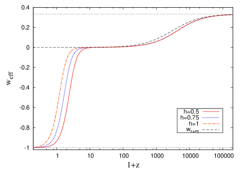
However, to obtain the results reported in Fig. 1, it was necessary to choose for a value which is clearly lower than the value obtained by WMAP 7. This is due to the fact that the HP also appears as a source of the DM.
We can perceive that, until the epoch of matter-radiation equality (approximately at ), the holographic fluid behaves as a relativistic component with , afterwards it behaves as a dustlike component, with , until it passes a redshift threshold () and begins to follow the asymptotic value . Moreover, in Fig. 1 we plotted the EoS parameter of the joint matter and radiation fluids, defined as
| (9) |
We can see that at high redshifts the behavior of the holographic fluid resembles that of the source fields. However, it is interesting to note that the effective EoS parameter departs from before that of the matter-radiation fluid. As we shall see in Sec. 5, this happens because the holographic fluids we consider are more likely to mimic matter fluids than relativistic ones.
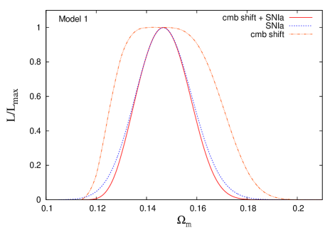
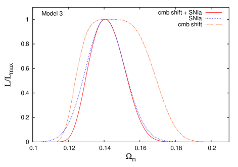
As first pointed out in the introduction, we suggest that both the DE and DM counterparts may be explained by the choice of the IR cutoff scale; so, to obtain a precise value for , we must perform a chi-squared fit with the supernovae union 2 data set Union2 and with the CMB shift parameter EstaBond . The combined test is sufficient to predict a specific value which will be tested further in Sec. V, where we will compare the predictions of our models with those of CDM, by using CMB anisotropies. All the remaining parameters, such as the Hubble constant, will be fixed by using the WMAP 7 maximum likelihood WMAP7y .
The application of the standard definition of the CMB shift EstaBond
| (10) |
presents some difficulties which can be overcome by using the alternative definition Melch
| (11) |
where is the position of the first peak on the CMB TT power spectrum of the model under consideration, and is the first peak in a flat FRW universe with . In particular, for approaches providing a unified description of both DE and DM, the latter expression must be used.
For any arbitrary model, is defined as
| (12) |
where is the comoving angular distance at recombination, i.e.,
| (13) |
and denotes the sound horizon at recombination
| (14) |
Here is the sound speed of the photon-to-baryon fluid, .
In the special case of CDM, the shift parameter is simplified to (10) due to the fact that the cosmological constant’s contribution to the Hubble flow is negligible for , so that it can be neglected in Eq. (14). In general this approximation is not valid. This is the case of the models that are the subject of this work. For these models, indeed, at early times the holographic fluid mimics the whole background’s fluids. Therefore we will deal hereafter with the definition (11).
The best value for the CMB shift parameter inferred from the WMAP7yr analysis is given by
| (15) |
On the other hand, for the supernovae (SNe) fit we compare the distance modulus
| (16) |
with the observational data of the Union 2 data set which encompasses 557 supernovae up to the redshift 1.7, which represents the highest value. Moreover, is the luminosity distance defined as
| (17) |
and then via WMAP data we set the Hubble parameter today as .
The results are summarized in Table 1. Figures 2 and Fig.3 show the likelihood functions of this analysis.
| Union 2 | CMB Shift | ShiftUnion2 | |
|---|---|---|---|
| () | |||
| Model 1 | |||
| (543.5) | |||
| Model 3 | |||
| (543.6) |
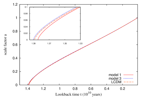
Fig. 4 shows, instead, the expansion history of the Universe for the best fits previously discussed, and the scale factor for the CDM model with the best fit parameter values given by WMAP 7 results WMAP7y . We note that there are slight differences that are more evident at early times. In other words, according to the above results, our models are able to describe the dynamics of the Universe by using a geometrical source for DM and DE, with small differences with respect to the CDM model at late times.
IV Low redshift regime: the Cosmography way
Cosmography is an additional tool to test a given model. Particularly, Cosmography represents a branch of cosmology, which promises insight into the cosmological picture, for exploring the kinematics of the Universe, without regards towards any a priori specific model, postulated in the Friedmann equations.
The kinematics is very useful to understand the expansion history of the Universe. First, as quoted, the kinematics does not depend on the choice of the model, second the kinematics can be directly fitted with the observable Universe, third it lies on the assumption that the cosmological quantities should be expanded in series around our time, , giving rise to easygoing relations. In this sense, naively, cosmography ingenuously builds on the simplest expediency to investigate the universe’s dynamics.
To apply cosmography one needs only the metric (5) that defines the geometry of the universe. In other words, it does not take into account any special modification of the Friedmann equations, independent of the choice of the model.
This policy was first mooted from Weinberg’s pioneering ideas. He suggested expanding the scale factor in series of powers, giving the possibility to relate it222Or the Hubble parameter, or the luminosity distances and so on. in terms of a Taylor series
where it is worthwhile to get the positions
| (19) | |||||
which are known in the literature as the deceleration parameter, the jerk parameter and the snap parameter, respectively. It is standard convention to assume that Eqs. (IV) represent the cosmographic set (CS), once each value has been evaluated at . Therefore, we commonly refer to the CS as the numerical values assumed by the above coefficients of the Taylor expansion at late time. Physically, this had to be argued since the series of has been evaluated around our time. Therefore, the luminosity distance can be rewritten as
Afterwards these expansions, we have all the instruments needed to perform a direct analysis. In fact, let us fit the Union 2 data compilation by Eq. (IV) in order to turn out experimental limits over and . Once the CS is known, it appears easy to invert them and to relate the free parameters of our models in terms of the CS. This guarantees experimental bounds on the previous models, giving us the possibility to establish whether our approaches work well or not in the low redshift regime.
IV.1 Experimental results
In order to perform a more stringent check on the reliability of the models, we test their predictions at low values of the redshift , by using the above results and those of Table I. In particular, we interrelate the theoretical features of our models with the CS by rewriting down in terms of the Hubble rate, i.e.
| (21) | |||||
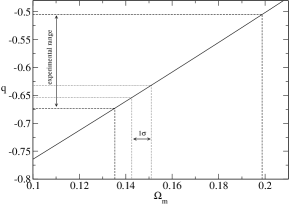
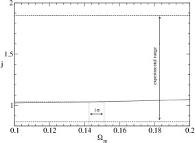
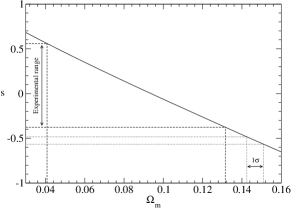
For consistency, we fix, for both models, the values of as in the previous section, and we develop the results shown in Figs. 5, 6 and 7, where we plot the values of , and , respectively, at as functions of for . In each plot, the dashed lines delimit the experimental range within the error bars and the corresponding interval of , while the dotted lines delimit the interval of confidence inferred from the expansion history analysis and the corresponding range of values of the cosmological parameters.
Notice that the values of and obtained for within the confidence interval are in agreement with the observations; only the parameter lies slightly outside the experimental range. The experimental ranges of the cosmological parameters and the values computed for within the confidence interval are written in tables 2 and 3 for the and , respectively. However, we refer to the experimental ranges as the numerical results that we obtained by fitting directly Eq. (IV) through the use of Union 2, while the theoretical results as the values obtained by inverting the CS in terms of using the values found in Table I for each model;
| Parameter | Experimental range | Theoretical range |
|---|---|---|
| q | -0.589 0.084 | |
| j | 1.359 0.518 | |
| s | 0.091 0.468 |
| Parameter | Experimental range | Theoretical range |
|---|---|---|
| q | -0.589 0.084 | |
| j | 1.359 0.518 | |
| s | 0.091 0.468 |
it follows from the two tables that both models are compatible with the experimental limits offered by Cosmography. Indeed, while excellently reproduces the experimental results, for the values of the cosmological parameters , , at , obtained for within the confidence interval, are not at the same agreement level as . An accurate look at the results shows that the goodness of remains disadvantaged, since it behaves worse than , which seems to appear more predictive, but it should not be ruled out definitively since the signs remain in the range of compatibility. Notice that the goodness offered by the cosmographic test actually reflects the intriguing physical aspect relying on the fact that in a low redshift regime we should expect that behaves like the CDM. In other words, we can expect that formerly reduces to a cosmological constant at small redshift more quickly than .
V Inhomogeneities and Anisotropies of the CMB power spectrum
In this section, we describe the imprint of anisotropies into the CMB power spectrum, by adopting our models and we develop the growth of inhomogeneities for the matter sector as well.
Since our models do not provide any analytical expressions for the anisotropic equations, we are trying to map both and by finding a suitable approximation to the expansion history for them. The basic idea is to map both the models, by using the results obtained in Sec. II, in order to check if they work at higher redshifts as well.
What we will immediately infer is that their behaviors suggest that the EoS can be approximated by three separated pieces, a dark matter fluid, a relativistic fluid and a cosmological constant term.
It turns out to be more accurate to perform this approximation, giving rise to an evolving EoS, precisely we follow the standard Chevallier-Polarski-Linder (CPL) parametrization CPLCP ; CPLL , which invokes as a barotropic factor the known expression .
Thus, we approximate the energy density of the holographic fluids () as
Here, the subscript stands for the holographic DM, mimicking the piece behaving as matter in the holographic EoS, while analogously represents the relativistic part, which mimics the relativistic term as well as the matter.
For purposes of CMB analysis we must demand a good approximation at early times, before recombination. A failure in the approximation at late times will be reflected in the large scale multipole moments () which are poorly constrained due to the cosmic variance.
For both models we adopt and WMAP7y and regarding , we assume the validity of the best fits given by SNeIa and CMB shift, found in Sec. III for each model.
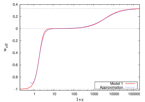
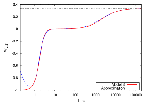
The numerical analysis shows that the compatible results are given by having for mod1: , , , , and fixed by the flat condition, e.g. . In Fig. 8 we plot the effective EoS parameter of mod1 under our approximation. It is well emphasized that the differences are extremely small, giving rise to good results of the first model at higher redshift. In particular, they have been estimated to be less than , before recombination ().
For mod3 analogously we have found , and . is again fixed by the requirement of spatially flat geometry like the above case. Figure 9 shows the effective EoS (weff) and the approximation based on the CPL parametrization. In this case, the differences are also small, being less than before recombination.
It appears intriguing to note that these approximations are not valid for future redshift, i.e. ; they cannot be extrapolated to the future.
Moreover, for both models the relativistic term behaves in the form , while for nonrelativistic matter we found . This definitively shows that the holographic models enhance the gravitational effects due to nonrelativistic fluids more than that of relativistic ones; we are not surprised by this feature, since, though in different ways, we have already anticipated it in Sec. III
In order to perform the power spectrum analysis, we proposed the use of the publicly available code CAMB Lewis00 ; in particular, we compare the holographic models with respect to the observational data and the CDM model as well.
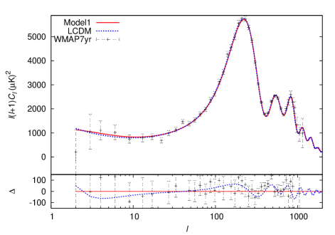
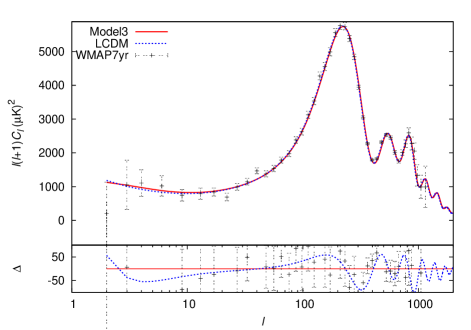
Figures 10 and Fig. 11 give the experimental results. In those figures, we plot the CMB TT angular power spectrum and the residual,
| (23) |
We elucidate great differences concentrated at large scales, which can be justified since the systematic errors due to the cosmic variance are strongly dominant. In addition, there are large discrepancies in the first three peaks, but these have been inferred to be well inside the error bars, different from the rest. At low scales, those differences quickly decay; this is as expected, because in the Silk damped tail region the anisotropies are mainly due to the microphysics driven by the photon-baryon plasma which the holographic fluid is not able to modify; indeed, the holographic fluids interact only gravitationally.
In order to obtain the plots of Figs. 10 and 11, we have also fixed the amplitude of the primordial scalar perturbation , defined as the proportionally constant in the equation
| (24) |
where is the primordial power spectrum of the gravitational potential , while , defined as the spectral index, is assumed to be and , where we moreover put an arbitrary pivotal scale in the above expression. For both holographic models and for CDM, which is used for calibrating our tests, we adopted respectively .
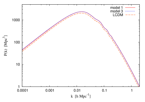
On the other hand, we emphasize that Fig. 12 shows the matter power spectrum of mod1;3; we found extremely small discrepancies between the three curves, where the third one is represented by CDM. The larger differences are located about , leaving probable imprints in the baryon acoustic oscillations that could be potentially detected in near future experiments. Nonetheless, currently these differences are not enough to discriminate between the CDM model and one of our models. This confirms that there is no reason not to use against the use of curvature invariants as a tool for explaining both DM and DE effects.
VI conclusion
In this work, we proposed as IR cutoff scale for the size , in the context of the cosmological HP, a second order geometrical approach, dealing with the use of independent invariants embedded in a FRW background, as a source for both DM and DE.
In particular, the DE density is assumed to be proportional to these invariants, which reduce from 14 to 3 in the FRW cosmology; thus, we use only GR and the HP to construct our models. Moreover, we extended the work of mio and we safely overcame the problem of causality, portrayed in cai , which represents one of the most serious shortcomings of the choice of the IR cutoff.
One of the main benefit of our approaches is basically due to the advantage of characterizing the acceleration of the Universe, by geometrical considerations only, by pointing out that the geometry is capable to describe the positive acceleration.
Particularly, we found two viable models (the third one is trivial, corresponding to the dustlike case only), and we developed a series of cosmological tests, able to explain their robustness. Therefore, the expansion history definitively fixed the values of and , the free parameters of our approaches, which have been described through the use of SNeIa and CMB tests.
Moreover, as a powerful analysis, we investigated cosmography in the framework of our models, since it has been testified an amusing interest on the Universe’s kinematics; the predictions of cosmography certified that is favored if compared to , as it has been pointed in Sec. III. We also arrived at analogous results in the last sections, with higher redshift tests. In fact, additional confirmation came from the direct study of the anisotropy of the power spectrum and then, after all, we conclude that our models can be pondered as possible sources of both DE and DM, becoming a viable candidate to explain unified schemes for the Universe’s dynamics; in particular, such a picture seems to be able to naturally reduce the problem of the DM presence in the Universe, in the framework of GR, being able to explain, at the same time, the cosmic speed up.
More considerations can be carried forward this idea, in order to check if, trough higher order invariants, it would be possible to definitively overcome the problem of DM and DE. This concept will be the object of future developments.
Acknowledgements
It is a pleasure to thank Dr. Andrea Geralico and Professor Salvatore Capozziello for very fruitful discussions.
References
- (1) M. W. Clifford, Physics, 4, 43, (2011).
- (2) A. G. Riess et al., AJ, 116, 1009, (1998)
- (3) S. Perlmutter et al., ApJ, 517, 565, (1999).
- (4) R. Rebolo et al., MNRAS, 353, 747, (2004); A. C. Pope et al., ApJ, 607, 655, (2004); P. McDonald et al., astro-ph/0405013, (2004); M. Tegmark et al. (SDSS), Phys. Rev. D74, 123507 (2006); W. J. Percival et al., Mon. Not. Roy. Astron. Soc. 381,1053, (2007).
- (5) E. J. Copeland, M. Sami, S. Tsujikawa, Int. J. Mod. Phys. D, 15, 1753-1936, (2006).
- (6) S. Weinberg, Cosmology, Oxford Univ. Press, Oxford, (2008); S. Weinberg, Rev. Mod. Phys. 61, 1, (1989).
- (7) S. Tsujikawa, ArXiv: 1004.1493.
- (8) M. Li, X. D. Li, S. Wang, Y. Wang, ArXiv: 1103.5870.
- (9) P. McFadden, K. Skenderis, Phys. Rev. D 81, 021301(R), (2010); R. Bousso, Rev. Mod. Phys.74:825-874, (2002).
- (10) Z. Chang, F. Q. Wu and X. Zhang, Phys. Lett. B 633, 14, (2006); B. Wang, C.Y. Lin and E. Abdalla, Phys. Lett. B 637, 357, (2006).
- (11) X. Zhang, Phys.Lett., B 648, 1, (2007); M. R. Setare, J. Zhang and X. Zhang, JCAP, 0703, 007, (2007); J. Zhang, X. Zhang and H. Liu, Phys. Lett. B 659, 26, (2008).
- (12) C.J. Feng, Phys. Lett. B, 633, 367, (2008);M. Li, X.D. Li, C. Lin and Y. Wang, Commun. Theor. Phys., 51, 181, (2009); M. Jamil, M. U. Farooq and M. A. Rashid, Eur. Phys. J. C, 61, 471, (2009).
- (13) L. Bonanno, G. Iannone, O. Luongo, ArXiv: 1101.5798.
- (14) R. G. Cai, Phys. Lett. B 657, 228, (2007).
- (15) C. Cherubini, D. Bini, S. Capozziello, R. Ruffini, Int. J. Mod. Phys. D,11, 827-841, (2002).
- (16) M. D. Roberts, Int. J. Mod. Phys., 9, 167, (1994).
- (17) J. Géhéniau and R. Debever, Bull. Cl. Sci. Acad. R. Belg. XLII, 114, (1956).
- (18) L. Witten, Phys. Rev., 113, 357, (1959).
- (19) A. Z. Petrov, Eistein Spaces, Pergamon, Oxford, (1969).
- (20) R. Penrose and W. Rindler, Spinors and Spacetime, Cambridge Univ. Press, (1986).
- (21) J. Carminati and R. G. McLenaghan, J. Math. Phys., 32, 3134, (1991).
- (22) Komatsu et al., Astrophys. J. Suppl. Ser. 192, 18 (2011). Larson et al., Astrophys. J. Suppl. Ser. 192, 16 (2011).
- (23) R. Amanullah et al., Astrophys. J. 716, 712 (2010).
- (24) J.R. Bond, G. Efstathiou and M. Tegmark, MNRAS 291 L33 (1997)
- (25) A. Melchiorri and L. M. Griffiths, New Astron.Rev. 45 321 (2001)
- (26) M. Chevalier and D. Polarski, Int. J. Mod. Phys. D., 10, 213,(2001).
- (27) E. Linder, Phys. Rev. Lett., 90, 091301, (2003).
- (28) A. Lewis, A. Challinor, and A. Lasenby, Astrophys. J 538, 473 (2000).