A Comparative Study of Dark Energy Constraints from Current Observational Data

YunΒ Wang1111email: wang@nhn.ou.edu, Chia-HsunΒ Chuang1, & PiaΒ Mukherjee2 1Homer L. Dodge Department of Physics & Astronomy, Univ. of Oklahoma, 440 W Brooks St., Norman, OK 73019
2Sussex Astronomy Centre, Dept. of Physics & Astronomy, University of Sussex, Falmer, Brighton, BN1 9QH, U.K.
Abstract

We examine how dark energy constraints from current observational data depend on the analysis methods used: the analysis of Type Ia supernovae (SNe Ia), and that of galaxy clustering data. We generalize the flux-averaging analysis method of SNe Ia to allow correlated errors of SNe Ia, in order to reduce the systematic bias due to weak lensing of SNe Ia. We find that flux-averaging leads to larger errors on dark energy and cosmological parameters if only SN Ia data are used. When SN Ia data (the latest compilation by the SNLS team) are combined with WMAP 7 year results (in terms of our Gaussian fits to the probability distributions of the CMB shift parameters), the latest Hubble constant (H0subscript𝐻0H_{0}) measurement using the Hubble Space Telescope (HST), and gamma ray burst (GRB) data, flux-averaging of SNe Ia increases the concordance with other data, and leads to significantly tighter constraints on the dark energy density at z=1𝑧1z=1, and the cosmic curvature Ξ©ksubscriptΞ©π‘˜\Omega_{k}. The galaxy clustering measurements of H​(z=0.35)​rs​(zd)𝐻𝑧0.35subscriptπ‘Ÿπ‘ subscript𝑧𝑑H(z=0.35)r_{s}(z_{d}) and rs​(zd)/DA​(z=0.35)subscriptπ‘Ÿπ‘ subscript𝑧𝑑subscript𝐷𝐴𝑧0.35r_{s}(z_{d})/D_{A}(z=0.35) (where H​(z)𝐻𝑧H(z) is the Hubble parameter, DA​(z)subscript𝐷𝐴𝑧D_{A}(z) is the angular diameter distance, and rs​(zd)subscriptπ‘Ÿπ‘ subscript𝑧𝑑r_{s}(z_{d}) is the sound horizon at the drag epoch) by Chuang & Wang (2011) are consistent with SN Ia data, given the same pirors (CMB+H0subscript𝐻0H_{0}+GRB), and lead to significantly improved dark energy constraints when combined. Current data are fully consistent with a cosmological constant and a flat universe.

Cosmology
pacs:
98.80.Es,98.80.-k,98.80.Jk

I Introduction

Solving the mystery of cosmic acceleration Riess et al. (1998); Perlmutter et al. (1999) is one of the most important challenges in cosmology today. Current observational data are not sufficient for differentiating two likely explanations for the observed cosmic acceleration: dark energy, and the modification of general relativity. For recent reviews, see Copeland06 ; Ruiz07 ; Ratra07 ; Frieman08 ; Caldwell09 ; Uzan09 ; Wang10 ; Li11 .

There are a number of powerful direct probes of dark energy: Type Ia supernovae (SNe Ia) Riess et al. (1998); Perlmutter et al. (1999); galaxy clustering (GC), especially the baryon acoustic oscillations (BAO) Blake & Glazebrook (2003); Seo & Eisenstein (2003); and weak lensing of galaxies Hu (2002); Jain & Taylor (2003). These methods are complementary to each other, and each method has its own systematic uncertainties. Other data, e.g., gamma ray bursts Amati02 ; Bloom, Frail, & Kulkarni (2003); Schaefer03 , can help strengthen the dark energy constraints.

The cosmic microwave background (CMB) anisotropy data provide strong priors on cosmological parameters (see, e.g., Komatsu et al. (2011)). Direct measurements on the Hubble constant (see, e.g., Riess et al. (2011)) also help break the degeneracy amongst the dark energy and cosmological parameters.

Much progress has been made since the discovery of cosmic acceleration in 1998. However, current data are still rather limited in constraining dark energy. In particular, different analysis methods of the same data could lead to significantly different constraints on dark energy. This is probably due to the fact that different methods have different residual systematic biases, and they often assume different priors on cosmological parameters as well.

In this paper we examine these issues by studying how dark energy constraints from current observational data depend on the analysis methods used. In particular, we explore the impact on the overall dark energy constraints of (1) using flux-averaging to minimize the weak lensing bias in the analysis of SNe Ia; (2) using radial and transverse distance constraints derived from GC data without assuming CMB priors.

We describe our method in Sec.II, present our results in Sec.III, and conclude in Sec.IV.

II Method

We only use methods that give geometric constraints on dark energy. The constraints on the growth rate of cosmic large scale structure are degenerate with the geometric constraints (see, e.g., Wang (2008a); Simpson & Peacock (2010)); current data do not allow the determination of both without strong assumptions, e.g., assuming that general relativity is not modified.

Geometric constraints on dark energy are derived from the measurement of distances. The comoving distance to an object at redshift z𝑧z is given by:

r​(z)=c​H0βˆ’1​|Ξ©k|βˆ’1/2​sinn​[|Ξ©k|1/2​Γ​(z)],π‘Ÿπ‘§π‘superscriptsubscript𝐻01superscriptsubscriptΞ©π‘˜12sinndelimited-[]superscriptsubscriptΞ©π‘˜12Γ𝑧\displaystyle r(z)=cH_{0}^{-1}\,|\Omega_{k}|^{-1/2}{\rm sinn}[|\Omega_{k}|^{1/2}\,\Gamma(z)], (1)
Γ​(z)=∫0zd​zβ€²E​(zβ€²),E​(z)=H​(z)/H0formulae-sequenceΓ𝑧superscriptsubscript0𝑧𝑑superscript𝑧′𝐸superscript𝑧′𝐸𝑧𝐻𝑧subscript𝐻0\displaystyle\Gamma(z)=\int_{0}^{z}\frac{dz^{\prime}}{E(z^{\prime})},\hskip 28.45274ptE(z)=H(z)/H_{0}

where sinn​(x)=sin⁑(x)sinnπ‘₯π‘₯{\rm sinn}(x)=\sin(x), xπ‘₯x, sinh⁑(x)π‘₯\sinh(x) for Ξ©k<0subscriptΞ©π‘˜0\Omega_{k}<0, Ξ©k=0subscriptΞ©π‘˜0\Omega_{k}=0, and Ξ©k>0subscriptΞ©π‘˜0\Omega_{k}>0 respectively; and the expansion rate of the universe H​(z)𝐻𝑧H(z) (i.e., the Hubble parameter) is given by

H2​(z)≑(aΛ™a)2superscript𝐻2𝑧superscriptΛ™π‘Žπ‘Ž2\displaystyle H^{2}(z)\equiv\left(\frac{\dot{a}}{a}\right)^{2}
=\displaystyle= H02​[Ξ©m​(1+z)3+Ξ©r​(1+z)4+Ξ©k​(1+z)2+Ξ©X​X​(z)],superscriptsubscript𝐻02delimited-[]subscriptΞ©π‘šsuperscript1𝑧3subscriptΞ©π‘Ÿsuperscript1𝑧4subscriptΞ©π‘˜superscript1𝑧2subscriptΩ𝑋𝑋𝑧\displaystyle H_{0}^{2}\left[\Omega_{m}(1+z)^{3}+\Omega_{r}(1+z)^{4}+\Omega_{k}(1+z)^{2}+\Omega_{X}X(z)\right],

where Ξ©m+Ξ©r+Ξ©k+Ξ©X=1subscriptΞ©π‘šsubscriptΞ©π‘ŸsubscriptΞ©π‘˜subscriptΩ𝑋1\Omega_{m}+\Omega_{r}+\Omega_{k}+\Omega_{X}=1, and the dark energy density function X​(z)𝑋𝑧X(z) is defined as

X​(z)≑ρX​(z)ρX​(0).𝑋𝑧subscriptπœŒπ‘‹π‘§subscriptπœŒπ‘‹0X(z)\equiv\frac{\rho_{X}(z)}{\rho_{X}(0)}. (3)

Note that Ξ©rβ‰ͺΞ©mmuch-less-thansubscriptΞ©π‘ŸsubscriptΞ©π‘š\Omega_{r}\ll\Omega_{m}, thus the Ξ©rsubscriptΞ©π‘Ÿ\Omega_{r} term is usually omitted in dark energy studies, since dark energy should only be important at late times.

II.1 Analysis of SN Ia Data

SN Ia data give measurements of the luminosity distance dL​(z)subscript𝑑𝐿𝑧d_{L}(z) through that of the distance modulus of each SN:

ΞΌ0≑mβˆ’M=5​log⁑[dL​(z)Mpc]+25,subscriptπœ‡0π‘šπ‘€5subscript𝑑𝐿𝑧Mpc25\mu_{0}\equiv m-M=5\log\left[\frac{d_{L}(z)}{\mathrm{Mpc}}\right]+25, (4)

where mπ‘šm and M𝑀M represent the apparent and absolute magnitude of a SN. The luminosity distance dL​(z)=(1+z)​r​(z)subscript𝑑𝐿𝑧1π‘§π‘Ÿπ‘§d_{L}(z)=(1+z)\,r(z), with the comoving distance r​(z)π‘Ÿπ‘§r(z) given by Eq.(1).

We use the compilation of SN Ia data by Conley et al. (2011) Conley11 , which include the SNe Ia from the first three years of the Supernova Legacy Survey (SNLS3), the largest homogeneous SN Ia data set. We compare two methods for using these SNe in constraining dark energy: with flux-averaging of SNe Ia, and without.

II.1.1 SN Ia Data

For a set of 472 SNe Ia, Conley et al. (2011) Conley11 give the apparent B𝐡B magnitude, mBsubscriptπ‘šπ΅m_{B}, and the covariance matrix for Δ​m≑mBβˆ’mmodΞ”π‘šsubscriptπ‘šπ΅subscriptπ‘šmod\Delta m\equiv m_{B}-m_{\rm mod}, with

mmod=5​log10β‘π’ŸL​(z|s)βˆ’Ξ±β€‹(sβˆ’1)+Ξ²β€‹π’ž+β„³,subscriptπ‘šmod5subscript10subscriptπ’ŸπΏconditional𝑧s𝛼𝑠1π›½π’žβ„³m_{\rm mod}=5\log_{10}{\cal D}_{L}(z|\mbox{\bf s})-\alpha(s-1)+\beta{\cal C}+{\cal M}, (5)

where π’ŸL​(z|s)subscriptπ’ŸπΏconditional𝑧s{\cal D}_{L}(z|\mbox{\bf s}) is the luminosity distance multiplied by H0subscript𝐻0H_{0} for a given set of cosmological parameters {𝐬}𝐬\{{\bf s}\}, s𝑠s is the stretch measure of the SN light curve shape, and π’žπ’ž{\cal C} is the color measure for the SN. β„³β„³{\cal M} is a nuisance parameter representing some combination of the absolute magnitude of a fiducial SN Ia, M𝑀M, and the Hubble constant H0subscript𝐻0H_{0}. Since the time dilation part of the observed luminosity distance depends on the total redshift zhelsubscript𝑧helz_{\rm hel} (special relativistic plus cosmological), we have Hui06

π’ŸL​(z|s)≑cβˆ’1​H0​(1+zhel)​r​(z|s),subscriptπ’ŸπΏconditional𝑧ssuperscript𝑐1subscript𝐻01subscript𝑧helπ‘Ÿconditional𝑧s{\cal D}_{L}(z|\mbox{\bf s})\equiv c^{-1}H_{0}(1+z_{\rm hel})r(z|\mbox{\bf s}), (6)

where z𝑧z and zhelsubscript𝑧helz_{\rm hel} are the CMB restframe and heliocentric redshifts of the SN.

For a set of N𝑁N SNe with correlated errors, we have Conley11

Ο‡2=Δ​mTβ‹…Cβˆ’1⋅Δ​msuperscriptπœ’2β‹…Ξ”superscriptm𝑇superscriptC1Ξ”m\chi^{2}=\Delta\mbox{\bf m}^{T}\cdot\mbox{\bf C}^{-1}\cdot\Delta\mbox{\bf m} (7)

where Δ​𝐦Δ𝐦\Delta\bf m is a vector with N𝑁N components, and C is the NΓ—N𝑁𝑁N\times N covariance matrix of the SNe Ia.

Note that Δ​mΞ”π‘š\Delta m is equivalent to Δ​μ0Ξ”subscriptπœ‡0\Delta\mu_{0}, since

Δ​m≑mBβˆ’mmod=[mB+α​(sβˆ’1)βˆ’Ξ²β€‹π’ž]βˆ’β„³.Ξ”π‘šsubscriptπ‘šπ΅subscriptπ‘šmoddelimited-[]subscriptπ‘šπ΅π›Όπ‘ 1π›½π’žβ„³\Delta m\equiv m_{B}-m_{\rm mod}=\left[m_{B}+\alpha(s-1)-\beta{\cal C}\right]-{\cal M}. (8)

The total covariance matrix is Conley11

C=Dstat+Cstat+Csys,CsubscriptDstatsubscriptCstatsubscriptCsys\mbox{\bf C}=\mbox{\bf D}_{\rm stat}+\mbox{\bf C}_{\rm stat}+\mbox{\bf C}_{\rm sys}, (9)

with the diagonal part of the statistical uncertainty given by Conley11

Dstat,iisubscriptDstatii\displaystyle\mbox{\bf D}_{\rm stat,ii} =\displaystyle= ΟƒmB,i2+Οƒint2+Οƒlensing2+Οƒhost​correction2subscriptsuperscript𝜎2subscriptπ‘šπ΅π‘–subscriptsuperscript𝜎2intsubscriptsuperscript𝜎2lensingsubscriptsuperscript𝜎2hostcorrection\displaystyle\sigma^{2}_{m_{B},i}+\sigma^{2}_{\rm int}+\sigma^{2}_{\rm lensing}+\sigma^{2}_{{\rm host}\,{\rm correction}} (10)
+[5​(1+zi)zi​(1+zi/2)​ln⁑10]2​σz,i2+Ξ±2​σs,i2+Ξ²2β€‹Οƒπ’ž,i2superscriptdelimited-[]51subscript𝑧𝑖subscript𝑧𝑖1subscript𝑧𝑖2102subscriptsuperscript𝜎2𝑧𝑖superscript𝛼2subscriptsuperscript𝜎2𝑠𝑖superscript𝛽2subscriptsuperscript𝜎2π’žπ‘–\displaystyle+\left[\frac{5(1+z_{i})}{z_{i}(1+z_{i}/2)\ln 10}\right]^{2}\sigma^{2}_{z,i}+\alpha^{2}\sigma^{2}_{s,i}+\beta^{2}\sigma^{2}_{{\cal C},i}
+2​α​CmB​s,iβˆ’2​β​CmBβ€‹π’ž,iβˆ’2​α​β​Csβ€‹π’ž,i,2𝛼subscript𝐢subscriptπ‘šπ΅π‘ π‘–2𝛽subscript𝐢subscriptπ‘šπ΅π’žπ‘–2𝛼𝛽subscriptπΆπ‘ π’žπ‘–\displaystyle+2\alpha C_{m_{B}s,i}-2\beta C_{m_{B}{\cal C},i}-2\alpha\beta C_{s{\cal C},i},

where CmB​s,isubscript𝐢subscriptπ‘šπ΅π‘ π‘–C_{m_{B}s,i}, CmBβ€‹π’ž,isubscript𝐢subscriptπ‘šπ΅π’žπ‘–C_{m_{B}{\cal C},i}, and Csβ€‹π’ž,isubscriptπΆπ‘ π’žπ‘–C_{s{\cal C},i} are the covariances between mBsubscriptπ‘šπ΅m_{B}, s𝑠s, and π’žπ’ž{\cal C} for the i𝑖i-th SN. Note also that Οƒz,i2subscriptsuperscript𝜎2𝑧𝑖\sigma^{2}_{z,i} includes a peculiar velocity residual of 0.0005 (i.e., 150 km/s) added in quadrature Conley11 .

The statistical and systematic covariance matrices, CstatsubscriptCstat\mbox{\bf C}_{\rm stat} and CsyssubscriptCsys\mbox{\bf C}_{\rm sys}, are generally not diagonal Conley11 , and are given in the form:

Cstat+Csys=V0+Ξ±2​Va+Ξ²2​Vb+2​α​V0​aβˆ’2​β​V0​bβˆ’2​α​β​Va​b.subscriptCstatsubscriptCsyssubscript𝑉0superscript𝛼2subscriptπ‘‰π‘Žsuperscript𝛽2subscript𝑉𝑏2𝛼subscript𝑉0π‘Ž2𝛽subscript𝑉0𝑏2𝛼𝛽subscriptπ‘‰π‘Žπ‘\mbox{\bf C}_{\rm stat}+\mbox{\bf C}_{\rm sys}=V_{0}+\alpha^{2}V_{a}+\beta^{2}V_{b}+2\alpha V_{0a}-2\beta V_{0b}-2\alpha\beta V_{ab}. (11)

where V0subscript𝑉0V_{0}, Vasubscriptπ‘‰π‘ŽV_{a}, Vbsubscript𝑉𝑏V_{b}, V0​asubscript𝑉0π‘ŽV_{0a}, V0​bsubscript𝑉0𝑏V_{0b}, and Va​bsubscriptπ‘‰π‘Žπ‘V_{ab} are matrices given by the SNLS data archive at https://tspace.library.utoronto.ca/handle/1807/24512/. CstatsubscriptCstat\mbox{\bf C}_{\rm stat} includes the uncertainty in the SN model. CsyssubscriptCsys\mbox{\bf C}_{\rm sys} includes the uncertainty in the zero point. Note that CstatsubscriptCstat\mbox{\bf C}_{\rm stat} and CsyssubscriptCsys\mbox{\bf C}_{\rm sys} do not depend on β„³β„³{\cal M}, since the relative distance moduli are independent of the value of β„³β„³{\cal M} Conley11 .

We refer the reader to Conley et al. (2011) Conley11 for a detailed discussion of the origins of the statistical and systematic errors. As an example, we note that the correlation of errors on different SNe arises from a statistical uncertainty in the zero point of one passband, e.g., rMsubscriptπ‘Ÿπ‘€r_{M}. This directly affects all SNe with rMsubscriptπ‘Ÿπ‘€r_{M} measurements due to K-corrections (restframe B𝐡B to rMsubscriptπ‘Ÿπ‘€r_{M}), and indirectly affects even the SNe without rMsubscriptπ‘Ÿπ‘€r_{M} measurements through the empirical SN models by changing the templates and the measured color-luminosity relationship.

II.1.2 The Recipe for Flux-Averaging of SNe Ia

Because we live in a lumpy universe, SN Ia observations can be misinterpreted if the effect of gravitational lensing is not properly accounted for (see, e.g., Clarkson11 ). Flux-averaging of SNe Ia was proposed to reduce the effect of the weak lensing of SNe Ia on cosmological parameter estimation Wang (2000). The basic idea is that because of flux conservation in gravitational lensing, the average magnification of a large number of SNe Ia at the same redshift should be unity. Thus averaging the observed flux from a large number of SNe Ia at the same redshift can recover the unlensed brightness of the SNe Ia at that redshift.

Wang & Mukherjee (2004) Wang & Mukherjee (2004) and Wang (2005) (Wang, 2005) developed a consistent framework for flux-averaging SNe Ia. Wang & Mukherjee (2004) Wang & Mukherjee (2004) gave the recipe for flux-averaging SNe Ia in the absence of correlated errors. Here we modify and generalize the recipe to allow correlated errors of SNe Ia.

As described in Wang (2000), the fluxes of SNe Ia in a redshift bin should only be averaged after removing their redshift dependence, which is a model-dependent process. For Ο‡2superscriptπœ’2\chi^{2} statistics using MCMC or a grid of parameters, here are the steps in flux-averaging:

(1) Convert the distance modulus of SNe Ia into β€œfluxes”,

F​(zl)≑10βˆ’(ΞΌ0data​(zl)βˆ’25)/2.5=(dLdata​(zl)Mpc)βˆ’2.𝐹subscript𝑧𝑙superscript10superscriptsubscriptπœ‡0datasubscript𝑧𝑙252.5superscriptsuperscriptsubscript𝑑𝐿datasubscript𝑧𝑙Mpc2F(z_{l})\equiv 10^{-(\mu_{0}^{\rm data}(z_{l})-25)/2.5}=\left(\frac{d_{L}^{\rm data}(z_{l})}{\mbox{Mpc}}\right)^{-2}. (12)

(2) For a given set of cosmological parameters {𝐬}𝐬\{{\bf s}\}, obtain β€œabsolute luminosities”, {ℒ​(zl)β„’subscript𝑧𝑙{\cal L}(z_{l})}, by removing the redshift dependence of the β€œfluxes”, i.e.,

ℒ​(zl)≑dL2​(zl|𝐬)​F​(zl).β„’subscript𝑧𝑙superscriptsubscript𝑑𝐿2conditionalsubscript𝑧𝑙𝐬𝐹subscript𝑧𝑙{\cal L}(z_{l})\equiv d_{L}^{2}(z_{l}|{\bf s})\,F(z_{l}). (13)

(3) Flux-average the β€œabsolute luminosities” {β„’lisubscriptsuperscriptℒ𝑖𝑙{\cal L}^{i}_{l}} in each redshift bin i𝑖i to obtain {β„’Β―i}superscript¯ℒ𝑖\left\{\overline{\cal L}^{i}\right\}:

β„’Β―i=1Niβ€‹βˆ‘l=1Niβ„’li​(zl(i)),ziΒ―=1Niβ€‹βˆ‘l=1Nizl(i).formulae-sequencesuperscript¯ℒ𝑖1subscript𝑁𝑖superscriptsubscript𝑙1subscript𝑁𝑖subscriptsuperscriptℒ𝑖𝑙subscriptsuperscript𝑧𝑖𝑙¯subscript𝑧𝑖1subscript𝑁𝑖superscriptsubscript𝑙1subscript𝑁𝑖subscriptsuperscript𝑧𝑖𝑙\overline{\cal L}^{i}=\frac{1}{N_{i}}\sum_{l=1}^{N_{i}}{\cal L}^{i}_{l}(z^{(i)}_{l}),\hskip 28.45274pt\overline{z_{i}}=\frac{1}{N_{i}}\sum_{l=1}^{N_{i}}z^{(i)}_{l}. (14)

(4) Place β„’Β―isuperscript¯ℒ𝑖\overline{\cal L}^{i} at the mean redshift zΒ―isubscript¯𝑧𝑖\overline{z}_{i} of the i𝑖i-th redshift bin, now the binned flux is

F¯​(zΒ―i)=β„’Β―i/dL2​(zΒ―i|s).¯𝐹subscript¯𝑧𝑖superscript¯ℒ𝑖superscriptsubscript𝑑𝐿2conditionalsubscript¯𝑧𝑖s\overline{F}(\overline{z}_{i})=\overline{\cal L}^{i}/d_{L}^{2}(\overline{z}_{i}|\mbox{\bf s}). (15)

(5) Compute the covariance matrix of F¯​(zΒ―i)¯𝐹subscript¯𝑧𝑖\overline{F}(\overline{z}_{i}) and F¯​(zΒ―j)¯𝐹subscript¯𝑧𝑗\overline{F}(\overline{z}_{j}):

Cov​[F¯​(zΒ―i),F¯​(zΒ―j)]Cov¯𝐹subscript¯𝑧𝑖¯𝐹subscript¯𝑧𝑗\displaystyle\mbox{Cov}\left[\overline{F}(\overline{z}_{i}),\overline{F}(\overline{z}_{j})\right]
=\displaystyle= 1Ni​Nj[ln⁑10/2.5dL​(zΒ―i|s)​dL​(zΒ―j|s)]2β‹…\displaystyle\frac{1}{N_{i}N_{j}}\left[\frac{\ln 10/2.5}{d_{L}(\overline{z}_{i}|\mbox{\bf s})d_{L}(\overline{z}_{j}|\mbox{\bf s})}\right]^{2}\cdot
βˆ‘l=1Niβˆ‘m=1Njℒ​(zl(i))​ℒ​(zm(j))β€‹βŸ¨Ξ”β€‹ΞΌ0data​(zl(i))​Δ​μ0data​(zm(j))⟩superscriptsubscript𝑙1subscript𝑁𝑖superscriptsubscriptπ‘š1subscript𝑁𝑗ℒsuperscriptsubscript𝑧𝑙𝑖ℒsuperscriptsubscriptπ‘§π‘šπ‘—delimited-βŸ¨βŸ©Ξ”superscriptsubscriptπœ‡0datasuperscriptsubscript𝑧𝑙𝑖Δsuperscriptsubscriptπœ‡0datasuperscriptsubscriptπ‘§π‘šπ‘—\displaystyle\sum_{l=1}^{N_{i}}\sum_{m=1}^{N_{j}}{\cal L}(z_{l}^{(i)}){\cal L}(z_{m}^{(j)})\langle\Delta\mu_{0}^{\rm data}(z_{l}^{(i)})\Delta\mu_{0}^{\rm data}(z_{m}^{(j)})\rangle

where βŸ¨Ξ”β€‹ΞΌ0data​(zl(i))​Δ​μ0data​(zm(j))⟩delimited-βŸ¨βŸ©Ξ”superscriptsubscriptπœ‡0datasuperscriptsubscript𝑧𝑙𝑖Δsuperscriptsubscriptπœ‡0datasuperscriptsubscriptπ‘§π‘šπ‘—\langle\Delta\mu_{0}^{\rm data}(z_{l}^{(i)})\Delta\mu_{0}^{\rm data}(z_{m}^{(j)})\rangle is the covariance of the measured distance moduli of the l𝑙l-th SN Ia in the i𝑖i-th redshift bin, and the mπ‘šm-th SN Ia in the j𝑗j-th redshift bin. ℒ​(z)ℒ𝑧{\cal L}(z) is defined by Eqs.(12) and (13).

(6) For the flux-averaged data, {F¯​(zΒ―i)}¯𝐹subscript¯𝑧𝑖\left\{\overline{F}(\overline{z}_{i})\right\}, compute

Ο‡2=βˆ‘i​jΔ​F¯​(zΒ―i)​Covβˆ’1​[F¯​(zΒ―i),F¯​(zΒ―j)]​Δ​F¯​(zΒ―j)superscriptπœ’2subscript𝑖𝑗Δ¯𝐹subscript¯𝑧𝑖superscriptCov1¯𝐹subscript¯𝑧𝑖¯𝐹subscript¯𝑧𝑗Δ¯𝐹subscript¯𝑧𝑗\chi^{2}=\sum_{ij}\Delta\overline{F}(\overline{z}_{i})\,\mbox{Cov}^{-1}\left[\overline{F}(\overline{z}_{i}),\overline{F}(\overline{z}_{j})\right]\,\Delta\overline{F}(\overline{z}_{j}) (17)

where

Δ​F¯​(zΒ―i)≑F¯​(zΒ―i)βˆ’Fp​(zΒ―i|s),Δ¯𝐹subscript¯𝑧𝑖¯𝐹subscript¯𝑧𝑖superscript𝐹𝑝conditionalsubscript¯𝑧𝑖s\Delta\overline{F}(\overline{z}_{i})\equiv\overline{F}(\overline{z}_{i})-F^{p}(\overline{z}_{i}|\mbox{\bf s}), (18)

with Fp​(zΒ―i|s)=(dL​(z|s)/Mpc)βˆ’2superscript𝐹𝑝conditionalsubscript¯𝑧𝑖ssuperscriptsubscript𝑑𝐿conditional𝑧sMpc2F^{p}(\overline{z}_{i}|\mbox{\bf s})=\left(d_{L}(z|\mbox{\bf s})/\mbox{Mpc}\right)^{-2}.

For the sample of SNe we use in this study, we flux-averaged the SNe with d​z=0.07𝑑𝑧0.07dz=0.07, to ensure that all redshift bins contain at least one SN. Our SN flux-averaging code is available at http://www.nhn.ou.edu/∼similar-to\simwang/SNcode/.

II.2 Galaxy Clustering Data

For GC data, we use the distance measurements from the SDSS DR7 data. We compare two sets of distance measurements from SDSS DR7: (1) β€œCW2”: the measurement of H​(z)​rs​(zd)𝐻𝑧subscriptπ‘Ÿπ‘ subscript𝑧𝑑H(z)r_{s}(z_{d}) and rs​(zd)/DA​(z)subscriptπ‘Ÿπ‘ subscript𝑧𝑑subscript𝐷𝐴𝑧r_{s}(z_{d})/D_{A}(z) (where H​(z)𝐻𝑧H(z) is the Hubble parameter, DA​(z)subscript𝐷𝐴𝑧D_{A}(z) is the angular diameter distance, and rs​(zd)subscriptπ‘Ÿπ‘ subscript𝑧𝑑r_{s}(z_{d}) is the sound horizon at the drag epoch) by Chuang & Wang (2011) CW11 from the two-dimensional two-point correlation function of SDSS DR7 Luminous Red Galaxies (LRGs); (2) β€œWP2”: the measurement of rs​(zd)/DV​(z=0.2)subscriptπ‘Ÿπ‘ subscript𝑧𝑑subscript𝐷𝑉𝑧0.2r_{s}(z_{d})/D_{V}(z=0.2) and rs​(zd)/DV​(z=0.35)subscriptπ‘Ÿπ‘ subscript𝑧𝑑subscript𝐷𝑉𝑧0.35r_{s}(z_{d})/D_{V}(z=0.35) (where DV​(z)subscript𝐷𝑉𝑧D_{V}(z) is the spherically-averaged distance) by Percival et al. (2010) Percival10 from the spherically-averaged power spectrum of combined data of SDSS DR7 LRG and main galaxy samples and 2-degree Field Galaxy Redshift Survey (2dFGRS).

Using the two-dimensional two-point correlation function of SDSS DR7 in the scale range of 40-120 Mpc/hβ„Žh, Chuang & Wang (2011) CW11 found that

H​(z=0.35)​rs​(zd)𝐻𝑧0.35subscriptπ‘Ÿπ‘ subscript𝑧𝑑\displaystyle H(z=0.35)r_{s}(z_{d}) =\displaystyle= 13020Β±530​km/s​(4%)plus-or-minus13020530kmspercent4\displaystyle 13020\pm 530\,{\rm km/s}\,\,(4\%)
rs​(zd)/DA​(z=0.35)subscriptπ‘Ÿπ‘ subscript𝑧𝑑subscript𝐷𝐴𝑧0.35\displaystyle r_{s}(z_{d})/D_{A}(z=0.35) =\displaystyle= 0.1518Β±0.0062​(4%)plus-or-minus0.15180.0062percent4\displaystyle 0.1518\pm 0.0062\,\,(4\%)
rπ‘Ÿ\displaystyle r =\displaystyle= βˆ’0.0584,0.0584\displaystyle-0.0584, (19)

where rπ‘Ÿr is the normalized correlation coefficient between H​(z=0.35)​rs​(zd)𝐻𝑧0.35subscriptπ‘Ÿπ‘ subscript𝑧𝑑H(z=0.35)r_{s}(z_{d}) and rs​(zd)/DA​(z=0.35)subscriptπ‘Ÿπ‘ subscript𝑧𝑑subscript𝐷𝐴𝑧0.35r_{s}(z_{d})/D_{A}(z=0.35), and rs​(zd)subscriptπ‘Ÿπ‘ subscript𝑧𝑑r_{s}(z_{d}) is the sound horizon at the drag epoch (given by Eqs.(28) and (32). The inverse covariance matrix of H​(z=0.35)​rs​(zd)𝐻𝑧0.35subscriptπ‘Ÿπ‘ subscript𝑧𝑑H(z=0.35)r_{s}(z_{d}) and rs​(zd)/DA​(z=0.35)subscriptπ‘Ÿπ‘ subscript𝑧𝑑subscript𝐷𝐴𝑧0.35r_{s}(z_{d})/D_{A}(z=0.35) is

CGC,CW2βˆ’1=(0.35722​Eβˆ’050.17833​Eβˆ’010.17833​Eβˆ’010.26104​E+05)superscriptsubscript𝐢GCCW210.35722𝐸050.17833𝐸010.17833𝐸010.26104𝐸05C_{\rm GC,CW2}^{-1}=\left(\begin{array}[]{cc}0.35722E-05&0.17833E-01\\ 0.17833E-01&0.26104E+05\end{array}\right) (20)

Spherically-averaged data give a measurement of dz≑rs​(zd)/DV​(z)subscript𝑑𝑧subscriptπ‘Ÿπ‘ subscript𝑧𝑑subscript𝐷𝑉𝑧d_{z}\equiv r_{s}(z_{d})/D_{V}(z), with

DV​(z)≑[r​(z)2​c​zH​(z)]1/3.subscript𝐷𝑉𝑧superscriptdelimited-[]π‘Ÿsuperscript𝑧2𝑐𝑧𝐻𝑧13D_{V}(z)\equiv\left[\frac{r(z)^{2}\,cz}{H(z)}\right]^{1/3}. (21)

Chuang & Wang (2011) found that

d0.35C​W≑rs​(zd)/DV​(z=0.35)=0.1161Β±0.0034​(2.9%)superscriptsubscript𝑑0.35πΆπ‘Šsubscriptπ‘Ÿπ‘ subscript𝑧𝑑subscript𝐷𝑉𝑧0.35plus-or-minus0.11610.0034percent2.9d_{0.35}^{CW}\equiv r_{s}(z_{d})/D_{V}(z=0.35)=0.1161\pm 0.0034\,\,(2.9\%) (22)

from the spherically-averaged correlation function of SDSS LRGs.

Using the spherically-averaged power spectrum of combined data of SDSS DR7 LRG and main galaxy samples and 2dFGRS, Percival et al. (2010) Percival10 found that

d0.2W​Psuperscriptsubscript𝑑0.2π‘Šπ‘ƒ\displaystyle d_{0.2}^{WP} ≑\displaystyle\equiv rs​(zd)/DV​(z=0.2)=0.1905Β±0.0061​(3.2%)subscriptπ‘Ÿπ‘ subscript𝑧𝑑subscript𝐷𝑉𝑧0.2plus-or-minus0.19050.0061percent3.2\displaystyle r_{s}(z_{d})/D_{V}(z=0.2)=0.1905\pm 0.0061\,\,(3.2\%)
d0.35W​Psuperscriptsubscript𝑑0.35π‘Šπ‘ƒ\displaystyle d_{0.35}^{WP} ≑\displaystyle\equiv rs​(zd)/DV​(z=0.35)=0.1097Β±0.0036​(3.3%)subscriptπ‘Ÿπ‘ subscript𝑧𝑑subscript𝐷𝑉𝑧0.35plus-or-minus0.10970.0036percent3.3\displaystyle r_{s}(z_{d})/D_{V}(z=0.35)=0.1097\pm 0.0036\,\,(3.3\%)
rπ‘Ÿ\displaystyle r =\displaystyle= 0.337,0.337\displaystyle 0.337, (23)

where rπ‘Ÿr is the normalized correlation coefficient of d0.2subscript𝑑0.2d_{0.2} and d0.35subscript𝑑0.35d_{0.35}. The inverse covariance matrix of (d0.2subscript𝑑0.2d_{0.2}, d0.35subscript𝑑0.35d_{0.35}) is Percival10

CGC,WPβˆ’1=(30124βˆ’17227βˆ’1722786977)superscriptsubscript𝐢GCWP130124172271722786977C_{\rm GC,WP}^{-1}=\left(\begin{array}[]{cc}30124&-17227\\ -17227&86977\end{array}\right) (24)

For comparison, we also consider the distance measurements from the WiggleZ survey at z=0.6𝑧0.6z=0.6 by Blake et al. (2011) Blake11 , and from the 6dF GRS at z=0.106𝑧0.106z=0.106 by Beutler et al. (2011) 6dF :

d0.6subscript𝑑0.6\displaystyle d_{0.6} ≑\displaystyle\equiv rs​(zd)/DV​(z=0.6)=0.0692Β±0.0033subscriptπ‘Ÿπ‘ subscript𝑧𝑑subscript𝐷𝑉𝑧0.6plus-or-minus0.06920.0033\displaystyle r_{s}(z_{d})/D_{V}(z=0.6)=0.0692\pm 0.0033
d0.106subscript𝑑0.106\displaystyle d_{0.106} ≑\displaystyle\equiv rs​(zd)/DV​(z=0.106)=0.336Β±0.015subscriptπ‘Ÿπ‘ subscript𝑧𝑑subscript𝐷𝑉𝑧0.106plus-or-minus0.3360.015\displaystyle r_{s}(z_{d})/D_{V}(z=0.106)=0.336\pm 0.015 (25)

GC data are included in our analysis by adding the following term to the Ο‡2superscriptπœ’2\chi^{2} of a given model with

Ο‡G​C2=Δ​pi​[CG​Cβˆ’1​(pi,pj)]​Δ​pj,Δ​pi=piβˆ’pid​a​t​a.formulae-sequencesubscriptsuperscriptπœ’2𝐺𝐢Δsubscript𝑝𝑖delimited-[]subscriptsuperscriptC1𝐺𝐢subscript𝑝𝑖subscript𝑝𝑗Δsubscript𝑝𝑗Δsubscript𝑝𝑖subscript𝑝𝑖superscriptsubscriptπ‘π‘–π‘‘π‘Žπ‘‘π‘Ž\chi^{2}_{GC}=\Delta p_{i}\left[{\rm C}^{-1}_{GC}(p_{i},p_{j})\right]\Delta p_{j},\hskip 14.22636pt\Delta p_{i}=p_{i}-p_{i}^{data}. (26)

For the Chuang & Wang (2011) GC measurements CW11 , p1=H​(z=0.35)​rs​(zd)subscript𝑝1𝐻𝑧0.35subscriptπ‘Ÿπ‘ subscript𝑧𝑑p_{1}=H(z=0.35)r_{s}(z_{d}) and p2=rs​(zd)/DA​(z=0.35)subscript𝑝2subscriptπ‘Ÿπ‘ subscript𝑧𝑑subscript𝐷𝐴𝑧0.35p_{2}=r_{s}(z_{d})/D_{A}(z=0.35). For the Percival et al. (2010) GC measurements Percival10 , p1=d0.2subscript𝑝1subscript𝑑0.2p_{1}=d_{0.2} and p2=d0.35subscript𝑝2subscript𝑑0.35p_{2}=d_{0.35}. Note that pid​a​t​asuperscriptsubscriptπ‘π‘–π‘‘π‘Žπ‘‘π‘Žp_{i}^{data} (i=1,2𝑖12i=1,2) are given in Eqs.(19) and (23), and the inverse covariance matrices are given in Eqs.(20) and (24). Since the WiggleZ and 6dF surveys give independent measurements, Eq.(26) is replaced with Ο‡G​C2=βˆ‘i=12(Δ​pi)2/Οƒpi2subscriptsuperscriptπœ’2𝐺𝐢superscriptsubscript𝑖12superscriptΞ”subscript𝑝𝑖2superscriptsubscript𝜎subscript𝑝𝑖2\chi^{2}_{GC}=\sum_{i=1}^{2}(\Delta p_{i})^{2}/\sigma_{p_{i}}^{2}, with p1=d0.6subscript𝑝1subscript𝑑0.6p_{1}=d_{0.6}, and p2=d0.106subscript𝑝2subscript𝑑0.106p_{2}=d_{0.106}, and Οƒpisubscript𝜎subscript𝑝𝑖\sigma_{p_{i}} (i=1,2𝑖12i=1,2) given in Eq.(II.2).

II.3 CMB data

CMB data give us the comoving distance to the photon-decoupling surface r​(zβˆ—)π‘Ÿsubscript𝑧r(z_{*}), and the comoving sound horizon at photo-decoupling epoch rs​(zβˆ—)subscriptπ‘Ÿπ‘ subscript𝑧r_{s}(z_{*}) Page (2003). Wang & Mukherjee 2007 Wang & Mukherjee (2007) showed that the CMB shift parameters

R𝑅\displaystyle R ≑\displaystyle\equiv Ξ©m​H02​r​(zβˆ—)/c,subscriptΞ©π‘šsuperscriptsubscript𝐻02π‘Ÿsubscript𝑧𝑐\displaystyle\sqrt{\Omega_{m}H_{0}^{2}}\,r(z_{*})/c,
lasubscriptπ‘™π‘Ž\displaystyle l_{a} ≑\displaystyle\equiv π​r​(zβˆ—)/rs​(zβˆ—),πœ‹π‘Ÿsubscript𝑧subscriptπ‘Ÿπ‘ subscript𝑧\displaystyle\pi r(z_{*})/r_{s}(z_{*}), (27)

together with Ο‰b≑Ωb​h2subscriptπœ”π‘subscriptΩ𝑏superscriptβ„Ž2\omega_{b}\equiv\Omega_{b}h^{2}, provide an efficient summary of CMB data as far as dark energy constraints go. This has been verified by Li08 . Replacing Ο‰bsubscriptπœ”π‘\omega_{b} with zβˆ—subscript𝑧z_{*} gives identical constraints when the CMB distance priors are combined with other data Wang08b .

The comoving sound horizon at redshift z𝑧z is given by

rs​(z)subscriptπ‘Ÿπ‘ π‘§\displaystyle r_{s}(z) =\displaystyle= ∫0tcs​d​tβ€²a=c​H0βˆ’1β€‹βˆ«zβˆžπ‘‘z′​csE​(zβ€²),superscriptsubscript0𝑑subscript𝑐𝑠𝑑superscriptπ‘‘β€²π‘Žπ‘superscriptsubscript𝐻01superscriptsubscript𝑧differential-dsuperscript𝑧′subscript𝑐𝑠𝐸superscript𝑧′\displaystyle\int_{0}^{t}\frac{c_{s}\,dt^{\prime}}{a}=cH_{0}^{-1}\int_{z}^{\infty}dz^{\prime}\,\frac{c_{s}}{E(z^{\prime})}, (28)
=\displaystyle= c​H0βˆ’1β€‹βˆ«0ad​aβ€²3​(1+Rb¯​aβ€²)​aβ€²4​E2​(zβ€²),𝑐superscriptsubscript𝐻01superscriptsubscript0π‘Žπ‘‘superscriptπ‘Žβ€²31Β―subscript𝑅𝑏superscriptπ‘Žβ€²superscriptsuperscriptπ‘Žβ€²4superscript𝐸2superscript𝑧′\displaystyle cH_{0}^{-1}\int_{0}^{a}\frac{da^{\prime}}{\sqrt{3(1+\overline{R_{b}}\,a^{\prime})\,{a^{\prime}}^{4}E^{2}(z^{\prime})}},

where aπ‘Ža is the cosmic scale factor, a=1/(1+z)π‘Ž11𝑧a=1/(1+z), and a4​E2​(z)=Ξ©m​(a+aeq)+Ξ©k​a2+Ξ©X​X​(z)​a4superscriptπ‘Ž4superscript𝐸2𝑧subscriptΞ©π‘šπ‘Žsubscriptπ‘ŽeqsubscriptΞ©π‘˜superscriptπ‘Ž2subscriptΩ𝑋𝑋𝑧superscriptπ‘Ž4a^{4}E^{2}(z)=\Omega_{m}(a+a_{\rm eq})+\Omega_{k}a^{2}+\Omega_{X}X(z)a^{4}, with aeq=Ξ©rad/Ξ©m=1/(1+zeq)subscriptπ‘ŽeqsubscriptΞ©radsubscriptΞ©π‘š11subscript𝑧eqa_{\rm eq}=\Omega_{\rm rad}/\Omega_{m}=1/(1+z_{\rm eq}), and zeq=2.5Γ—104​Ωm​h2​(TC​M​B/2.7​K)βˆ’4subscript𝑧eq2.5superscript104subscriptΞ©π‘šsuperscriptβ„Ž2superscriptsubscript𝑇𝐢𝑀𝐡2.7K4z_{\rm eq}=2.5\times 10^{4}\Omega_{m}h^{2}(T_{CMB}/2.7\,{\rm K})^{-4}. The sound speed is cs=1/3​(1+Rb¯​a)subscript𝑐𝑠131Β―subscriptπ‘…π‘π‘Žc_{s}=1/\sqrt{3(1+\overline{R_{b}}\,a)}, with Rb¯​a=3​ρb/(4​ργ)Β―subscriptπ‘…π‘π‘Ž3subscriptπœŒπ‘4subscriptπœŒπ›Ύ\overline{R_{b}}\,a=3\rho_{b}/(4\rho_{\gamma}), RbΒ―=31500​Ωb​h2​(TC​M​B/2.7​K)βˆ’4Β―subscript𝑅𝑏31500subscriptΩ𝑏superscriptβ„Ž2superscriptsubscript𝑇𝐢𝑀𝐡2.7K4\overline{R_{b}}=31500\Omega_{b}h^{2}(T_{CMB}/2.7\,{\rm K})^{-4}. We take TC​M​B=2.725subscript𝑇𝐢𝑀𝐡2.725T_{CMB}=2.725.

The redshift to the photon-decoupling surface, zβˆ—subscript𝑧z_{*}, is given by the fitting formula Hu & Sugiyama (1996):

zβˆ—=1048​[1+0.00124​(Ξ©b​h2)βˆ’0.738]​[1+g1​(Ξ©m​h2)g2],subscript𝑧1048delimited-[]10.00124superscriptsubscriptΩ𝑏superscriptβ„Ž20.738delimited-[]1subscript𝑔1superscriptsubscriptΞ©π‘šsuperscriptβ„Ž2subscript𝑔2z_{*}=1048\,\left[1+0.00124(\Omega_{b}h^{2})^{-0.738}\right]\,\left[1+g_{1}(\Omega_{m}h^{2})^{g_{2}}\right], (29)

where

g1subscript𝑔1\displaystyle g_{1} =\displaystyle= 0.0783​(Ξ©b​h2)βˆ’0.2381+39.5​(Ξ©b​h2)0.7630.0783superscriptsubscriptΩ𝑏superscriptβ„Ž20.238139.5superscriptsubscriptΩ𝑏superscriptβ„Ž20.763\displaystyle\frac{0.0783\,(\Omega_{b}h^{2})^{-0.238}}{1+39.5\,(\Omega_{b}h^{2})^{0.763}} (30)
g2subscript𝑔2\displaystyle g_{2} =\displaystyle= 0.5601+21.1​(Ξ©b​h2)1.810.560121.1superscriptsubscriptΩ𝑏superscriptβ„Ž21.81\displaystyle\frac{0.560}{1+21.1\,(\Omega_{b}h^{2})^{1.81}} (31)

The redshift of the drag epoch zdsubscript𝑧𝑑z_{d} is well approximated by Eisenstein & Hu (1998)

zd=1291​(Ξ©m​h2)0.2511+0.659​(Ξ©m​h2)0.828​[1+b1​(Ξ©b​h2)b​2],subscript𝑧𝑑1291superscriptsubscriptΞ©π‘šsuperscriptβ„Ž20.25110.659superscriptsubscriptΞ©π‘šsuperscriptβ„Ž20.828delimited-[]1subscript𝑏1superscriptsubscriptΩ𝑏superscriptβ„Ž2𝑏2z_{d}=\frac{1291(\Omega_{m}h^{2})^{0.251}}{1+0.659(\Omega_{m}h^{2})^{0.828}}\left[1+b_{1}(\Omega_{b}h^{2})^{b2}\right], (32)

where

b1subscript𝑏1\displaystyle b_{1} =\displaystyle= 0.313​(Ξ©m​h2)βˆ’0.419​[1+0.607​(Ξ©m​h2)0.674],0.313superscriptsubscriptΞ©π‘šsuperscriptβ„Ž20.419delimited-[]10.607superscriptsubscriptΞ©π‘šsuperscriptβ„Ž20.674\displaystyle 0.313(\Omega_{m}h^{2})^{-0.419}\left[1+0.607(\Omega_{m}h^{2})^{0.674}\right], (33)
b2subscript𝑏2\displaystyle b_{2} =\displaystyle= 0.238​(Ξ©m​h2)0.223.0.238superscriptsubscriptΞ©π‘šsuperscriptβ„Ž20.223\displaystyle 0.238(\Omega_{m}h^{2})^{0.223}. (34)

We have derived the one-dimensional marginalized probability distributions (pdf) of (la,R,zβˆ—,ns,rs​(zd))subscriptπ‘™π‘Žπ‘…subscript𝑧subscript𝑛𝑠subscriptπ‘Ÿπ‘ subscript𝑧𝑑(l_{a},R,z_{*},n_{s},r_{s}(z_{d})) from WMAP7 data, for three different assumptions about dark energy: (1) wX​(z)=βˆ’1subscript𝑀𝑋𝑧1w_{X}(z)=-1; (2) wX​(z)=wsubscript𝑀𝑋𝑧𝑀w_{X}(z)=w (constant); (3) wX​(z)=w0+wa​(1βˆ’a)subscript𝑀𝑋𝑧subscript𝑀0subscriptπ‘€π‘Ž1π‘Žw_{X}(z)=w_{0}+w_{a}(1-a) Chev01 (2001). We find that these pdf’s are nearly independent of the assumption about dark energy, and are well fitted by Gaussian distributions with the following means and standard deviations:

⟨la⟩=302.35,σ​(la)=0.86formulae-sequencedelimited-⟨⟩subscriptπ‘™π‘Ž302.35𝜎subscriptπ‘™π‘Ž0.86\displaystyle\langle l_{a}\rangle=302.35,\sigma(l_{a})=0.86
⟨R⟩=1.728,σ​(R)=0.02formulae-sequencedelimited-βŸ¨βŸ©π‘…1.728πœŽπ‘…0.02\displaystyle\langle R\rangle=1.728,\sigma(R)=0.02
⟨zβˆ—βŸ©=1091.32,σ​(zβˆ—)=1.0formulae-sequencedelimited-⟨⟩subscript𝑧1091.32𝜎subscript𝑧1.0\displaystyle\langle z_{*}\rangle=1091.32,\sigma(z_{*})=1.0
⟨ns⟩=0.963,σ​(ns)=0.016formulae-sequencedelimited-⟨⟩subscript𝑛𝑠0.963𝜎subscript𝑛𝑠0.016\displaystyle\langle n_{s}\rangle=0.963,\sigma(n_{s})=0.016
⟨rs​(zd)⟩=152.85​Mpc,σ​(rs​[zd])=1.85​Mpc.formulae-sequencedelimited-⟨⟩subscriptπ‘Ÿπ‘ subscript𝑧𝑑152.85Mpc𝜎subscriptπ‘Ÿπ‘ delimited-[]subscript𝑧𝑑1.85Mpc\displaystyle\langle r_{s}(z_{d})\rangle=152.85\,{\rm Mpc},\sigma(r_{s}[z_{d}])=1.85\,{\rm Mpc}. (35)

Our Gaussian fits are fully consistent with the bestfit values for a constant w𝑀w from Komatsu’s website Komatsu10 .

The normalized covariance matrix of (la,R,zβˆ—,ns,rs​(zd))subscriptπ‘™π‘Žπ‘…subscript𝑧subscript𝑛𝑠subscriptπ‘Ÿπ‘ subscript𝑧𝑑(l_{a},R,z_{*},n_{s},r_{s}(z_{d})) is

(1.0000.20794.47422βˆ’.54889.34914.207941.0000.74409βˆ’.44370βˆ’.76929.47422.744091.0000βˆ’.79575βˆ’.19121βˆ’.54889βˆ’.44370βˆ’.795751.0000βˆ’.09973.34914βˆ’.76929βˆ’.19121βˆ’.099731.0000)1.0000.20794.47422.54889.34914.207941.0000.74409.44370.76929.47422.744091.0000.79575.19121.54889.44370.795751.0000.09973.34914.76929.19121.099731.0000\left(\begin{array}[]{ccccc}1.0000&.20794&.47422&-.54889&.34914\\ .20794&1.0000&.74409&-.44370&-.76929\\ .47422&.74409&1.0000&-.79575&-.19121\\ -.54889&-.44370&-.79575&1.0000&-.09973\\ .34914&-.76929&-.19121&-.09973&1.0000\end{array}\right) (36)

We find that the addition of rs​(zd)subscriptπ‘Ÿπ‘ subscript𝑧𝑑r_{s}(z_{d}) is redundant, and amounts to partially double-weighting the CMB constraints; so its measurement cannot be used in the CMB priors unless it is used to replace la​(zβˆ—)subscriptπ‘™π‘Žsubscript𝑧l_{a}(z_{*}). This was not apparent when WMAP5 data were used Wang09 ; this is because WMAP7 data provide significantly tighter constraints on the set of CMB distance priors.

Since the primary GC data we use in this paper have been marginalized over nssubscript𝑛𝑠n_{s} CW11 , we should marginalized the CMB distance priors over nssubscript𝑛𝑠n_{s} as well. When marginalized over nssubscript𝑛𝑠n_{s} and rs​(zd)subscriptπ‘Ÿπ‘ subscript𝑧𝑑r_{s}(z_{d}), the inverse covariance matrix of (la,R,zβˆ—)subscriptπ‘™π‘Žπ‘…subscript𝑧(l_{a},R,z_{*}) from WMAP7 is

CovC​M​Bβˆ’1=(1.857125.929βˆ’1.143325.9295963.3βˆ’99.319βˆ’1.1433βˆ’99.3192.9443)superscriptsubscriptCov𝐢𝑀𝐡11.857125.9291.143325.9295963.399.3191.143399.3192.9443\mbox{Cov}_{CMB}^{-1}=\left(\begin{array}[]{ccc}1.8571&25.929&-1.1433\\ 25.929&5963.3&-99.319\\ -1.1433&-99.319&2.9443\end{array}\right) (37)

CMB data are included in our analysis by adding the following term to the Ο‡2superscriptπœ’2\chi^{2} of a given model with p1=la​(zβˆ—)subscript𝑝1subscriptπ‘™π‘Žsubscript𝑧p_{1}=l_{a}(z_{*}), p2=R​(zβˆ—)subscript𝑝2𝑅subscript𝑧p_{2}=R(z_{*}),and p3=zβˆ—subscript𝑝3subscript𝑧p_{3}=z_{*}:

Ο‡C​M​B2=Δ​pi​[CovC​M​Bβˆ’1​(pi,pj)]​Δ​pj,Δ​pi=piβˆ’pid​a​t​a,formulae-sequencesubscriptsuperscriptπœ’2𝐢𝑀𝐡Δsubscript𝑝𝑖delimited-[]subscriptsuperscriptCov1𝐢𝑀𝐡subscript𝑝𝑖subscript𝑝𝑗Δsubscript𝑝𝑗Δsubscript𝑝𝑖subscript𝑝𝑖superscriptsubscriptπ‘π‘–π‘‘π‘Žπ‘‘π‘Ž\chi^{2}_{CMB}=\Delta p_{i}\left[\mbox{Cov}^{-1}_{CMB}(p_{i},p_{j})\right]\Delta p_{j},\hskip 14.22636pt\Delta p_{i}=p_{i}-p_{i}^{data}, (38)

where pid​a​t​asuperscriptsubscriptπ‘π‘–π‘‘π‘Žπ‘‘π‘Žp_{i}^{data} are the mean from Eq.(35), and CovC​M​Bβˆ’1subscriptsuperscriptCov1𝐢𝑀𝐡{\rm Cov}^{-1}_{CMB} is the inverse covariance matrix of [R(zβˆ—),la(zβˆ—),zβˆ—]R(z_{*}),l_{a}(z_{*}),z_{*}] from Eq.(37). Note that p4=nssubscript𝑝4subscript𝑛𝑠p_{4}=n_{s} should be added if the constraints on nssubscript𝑛𝑠n_{s} are included in the GC data. Finally, our Gaussian fit for the pdf of rs​(zd)subscriptπ‘Ÿπ‘ subscript𝑧𝑑r_{s}(z_{d}) should be useful when fitting for BAO peak locations.

II.4 Gammay-ray Burst Data

We add gammay-ray burst (GRB) data to our analysis, since these are complementary in redshift range to the SN Ia data. We use GRB data in the form of the model-independent GRB distance measurements from Wang (2008c) Wang08c , which were derived from the data of 69 GRBs with 0.17≀z≀6.60.17𝑧6.60.17\leq z\leq 6.6 from Schaefer (2007) Schaefer07 222The proper calibration of GRBs is an active area of research. For recent studies on the impact of detector thresholds, spectral analysis, and unknown selection effects, see, e.g., Butler07 ; Butler09 ; Petrosian09 ; Shahmoradi11 ..

The GRB distance measurements are given in terms of Wang08c

rp¯​(zi)≑rp​(z)rp​(0.17),rp​(z)≑(1+z)1/2z​H0c​h​r​(z),formulae-sequenceΒ―subscriptπ‘Ÿπ‘subscript𝑧𝑖subscriptπ‘Ÿπ‘π‘§subscriptπ‘Ÿπ‘0.17subscriptπ‘Ÿπ‘π‘§superscript1𝑧12𝑧subscript𝐻0π‘β„Žπ‘Ÿπ‘§\overline{r_{p}}(z_{i})\equiv\frac{r_{p}(z)}{r_{p}(0.17)},\hskip 28.45274ptr_{p}(z)\equiv\frac{(1+z)^{1/2}}{z}\,\frac{H_{0}}{ch}\,r(z), (39)

where r​(z)π‘Ÿπ‘§r(z) is the comoving distance at z𝑧z.

The GRB data are included in our analysis by adding the following term to the Ο‡2superscriptπœ’2\chi^{2} of a given model:

Ο‡G​R​B2subscriptsuperscriptπœ’2𝐺𝑅𝐡\displaystyle\chi^{2}_{GRB} =\displaystyle= [Δ​rp¯​(zi)]β‹…(CovG​R​Bβˆ’1)i​jβ‹…[Δ​rp¯​(zj)]β‹…delimited-[]Δ¯subscriptπ‘Ÿπ‘subscript𝑧𝑖subscriptsubscriptsuperscriptCov1𝐺𝑅𝐡𝑖𝑗delimited-[]Δ¯subscriptπ‘Ÿπ‘subscript𝑧𝑗\displaystyle\left[\Delta\overline{r_{p}}(z_{i})\right]\cdot\left(\mathrm{Cov}^{-1}_{GRB}\right)_{ij}\cdot\left[\Delta\overline{r_{p}}(z_{j})\right]
Δ​rp¯​(zi)Δ¯subscriptπ‘Ÿπ‘subscript𝑧𝑖\displaystyle\Delta\overline{r_{p}}(z_{i}) =\displaystyle= rpΒ―data​(zi)βˆ’rp¯​(zi),superscriptΒ―subscriptπ‘Ÿπ‘datasubscript𝑧𝑖¯subscriptπ‘Ÿπ‘subscript𝑧𝑖\displaystyle\overline{r_{p}}^{\mathrm{data}}(z_{i})-\overline{r_{p}}(z_{i}), (40)

where rp¯​(z)Β―subscriptπ‘Ÿπ‘π‘§\overline{r_{p}}(z) is defined by Eq.(39). The covariance matrix is given by

(CovG​R​B)i​j=σ​(rp¯​(zi))​σ​(rp¯​(zj))​(CovΒ―G​R​B)i​j,subscriptsubscriptCovπΊπ‘…π΅π‘–π‘—πœŽΒ―subscriptπ‘Ÿπ‘subscriptπ‘§π‘–πœŽΒ―subscriptπ‘Ÿπ‘subscript𝑧𝑗subscriptsubscriptΒ―Cov𝐺𝑅𝐡𝑖𝑗\left(\mathrm{Cov}_{GRB}\right)_{ij}=\sigma(\overline{r_{p}}(z_{i}))\sigma(\overline{r_{p}}(z_{j}))\left(\overline{\mathrm{Cov}}_{GRB}\right)_{ij}, (41)

where CovΒ―G​R​BsubscriptΒ―Cov𝐺𝑅𝐡\overline{\mathrm{Cov}}_{GRB} is the normalized covariance matrix from Table 3 of Wang (2008c) Wang08c , and

σ​(rp¯​(zi))𝜎¯subscriptπ‘Ÿπ‘subscript𝑧𝑖\displaystyle\sigma(\overline{r_{p}}(z_{i})) =\displaystyle= σ​(rp¯​(zi))+,if​rp¯​(z)β‰₯rp¯​(z)data;𝜎superscriptΒ―subscriptπ‘Ÿπ‘subscript𝑧𝑖ifΒ―subscriptπ‘Ÿπ‘π‘§Β―subscriptπ‘Ÿπ‘superscript𝑧data\displaystyle\sigma\left(\overline{r_{p}}(z_{i})\right)^{+},\hskip 14.22636pt\mathrm{if}\,\,\overline{r_{p}}(z)\geq\overline{r_{p}}(z)^{\mathrm{data}};
σ​(rp¯​(zi))𝜎¯subscriptπ‘Ÿπ‘subscript𝑧𝑖\displaystyle\sigma(\overline{r_{p}}(z_{i})) =\displaystyle= σ​(rp¯​(zi))βˆ’,if​rp¯​(z)<rp¯​(z)data,𝜎superscriptΒ―subscriptπ‘Ÿπ‘subscript𝑧𝑖ifΒ―subscriptπ‘Ÿπ‘π‘§Β―subscriptπ‘Ÿπ‘superscript𝑧data\displaystyle\sigma\left(\overline{r_{p}}(z_{i})\right)^{-},\hskip 14.22636pt\mathrm{if}\,\,\overline{r_{p}}(z)<\overline{r_{p}}(z)^{\mathrm{data}}, (42)

where σ​(rp¯​(zi))+𝜎superscriptΒ―subscriptπ‘Ÿπ‘subscript𝑧𝑖\sigma\left(\overline{r_{p}}(z_{i})\right)^{+} and σ​(rp¯​(zi))βˆ’πœŽsuperscriptΒ―subscriptπ‘Ÿπ‘subscript𝑧𝑖\sigma\left(\overline{r_{p}}(z_{i})\right)^{-} are the 68% C.L. errors given in Table 2 of Wang (2008c) Wang08c .

II.5 Dark energy parametrization

Since we are ignorant of the true nature of dark energy, it is useful to measure the dark energy density function X​(z)≑ρX​(z)/ρX​(0)𝑋𝑧subscriptπœŒπ‘‹π‘§subscriptπœŒπ‘‹0X(z)\equiv\rho_{X}(z)/\rho_{X}(0) as a free function of redshift Wang & Garnavich (2001); Wang & Tegmark (2004); Wang & Freese (2006). This has the advantage of allowing dark energy models in which ρX​(z)subscriptπœŒπ‘‹π‘§\rho_{X}(z) becomes negative in the future, e.g., the β€œBig Crunch” models Linde (1987); WangLinde04 , which are precluded if we parametrize dark energy with an equation of state wX​(z)subscript𝑀𝑋𝑧w_{X}(z) Wang & Tegmark (2004).

Here we parametrize X​(z)𝑋𝑧X(z) by cubic-splining its values at z=1/3𝑧13z=1/3, 2/3232/3, and 1.0, and assume that X​(z>1)=X​(z=1)𝑋𝑧1𝑋𝑧1X(z>1)=X(z=1). For simplicity of notation, we define X0.33≑X​(z=1/3)subscript𝑋0.33𝑋𝑧13X_{0.33}\equiv X(z=1/3), X0.67≑X​(z=2/3)subscript𝑋0.67𝑋𝑧23X_{0.67}\equiv X(z=2/3), and X1.0≑X​(z=1)subscript𝑋1.0𝑋𝑧1X_{1.0}\equiv X(z=1). Fixing X​(z>1)𝑋𝑧1X(z>1) reflects the limit of current data, and avoids making assumptions about early dark energy that can be propagated into artificial constraints on dark energy at low z𝑧z Wang & Tegmark (2004); Wang & Mukherjee (2007).

For comparison with the work of others, we also consider a dark energy equation of state linear in the cosmic scale factor aπ‘Ža, wX​(a)=w0+(1βˆ’a)​wasubscriptπ‘€π‘‹π‘Žsubscript𝑀01π‘Žsubscriptπ‘€π‘Žw_{X}(a)=w_{0}+(1-a)w_{a} Chev01 (2001). A related parametrization is Wang08b

wX​(z)=w0​(3​aβˆ’2)+3​w0.5​(1βˆ’a),subscript𝑀𝑋𝑧subscript𝑀03π‘Ž23subscript𝑀0.51π‘Žw_{X}(z)=w_{0}(3a-2)+3w_{0.5}(1-a), (43)

where w0.5≑wX​(z=0.5)subscript𝑀0.5subscript𝑀𝑋𝑧0.5w_{0.5}\equiv w_{X}(z=0.5). Wang (2008b) Wang08b showed that (w0subscript𝑀0w_{0}, w0.5subscript𝑀0.5w_{0.5}) are much less correlated than (w0subscript𝑀0w_{0}, wasubscriptπ‘€π‘Žw_{a}), thus are a better set of parameters to use. We find that (w0subscript𝑀0w_{0}, w0.5subscript𝑀0.5w_{0.5}) converge much faster than (w0subscript𝑀0w_{0}, wasubscriptπ‘€π‘Žw_{a}) in a Markov Chain Monte Carlo (MCMC) likelihood analysis for the same data.

III Results

We perform a MCMC likelihood analysis Lewis02 (2002) to obtain π’ͺπ’ͺ{\cal O}(106superscript10610^{6}) samples for each set of results presented in this paper. We assume flat priors for all the parameters, and allow ranges of the parameters wide enough such that further increasing the allowed ranges has no impact on the results. The chains typically have worst e-values, defined to be the variance(mean)/mean(variance) of 1/2 chains, much smaller than 0.005, indicating convergence. The chains are subsequently appropriately thinned to ensure independent samples.

In addition to the SN Ia, CMB, GC, and GRB data discussed in Sec.II, we impose a prior of H0=73.8Β±2.4subscript𝐻0plus-or-minus73.82.4H_{0}=73.8\pm 2.4\,km s-1Mpc-1, from the HST measurements by Riess et al. (2011) Riess et al. (2011).

We do not assume a flat universe unless specifically noted. In addition to the dark energy parameters described in Sec.II.5, we also constrain cosmological parameters (Ξ©m,Ξ©k,h,Ο‰bsubscriptΞ©π‘šsubscriptΞ©π‘˜β„Žsubscriptπœ”π‘\Omega_{m},\Omega_{k},h,\omega_{b}), where Ο‰b≑Ωb​h2subscriptπœ”π‘subscriptΩ𝑏superscriptβ„Ž2\omega_{b}\equiv\Omega_{b}h^{2}. In addition, we marginalize over the SN Ia nuisance parameters {Ξ±,Ξ²,β„³}𝛼𝛽ℳ\{\alpha,\beta,{\cal M}\}.

We will present results for dark energy density at z=1/3𝑧13z=1/3, 2/3232/3, and 1, as well as (w0,wasubscript𝑀0subscriptπ‘€π‘Žw_{0},w_{a}) and (w0,w0.5subscript𝑀0subscript𝑀0.5w_{0},w_{0.5}), and a constant dark energy equation of state w𝑀w.

III.1 The effect of flux-averaging of SNe Ia

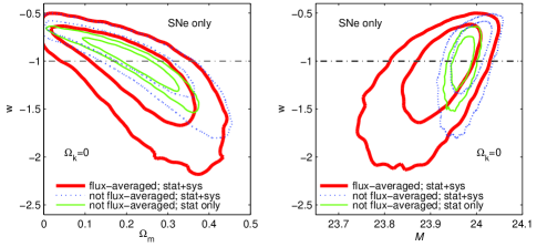
Figs.1 shows the 2D marginalized contours of (w,Ξ©m,β„³)𝑀subscriptΞ©π‘šβ„³(w,\Omega_{m},{\cal M}), assuming a constant equation of state for dark energy, w𝑀w, and a flat universe. Note that the inclusion of systematic errors of SNe leads to significantly larger uncertainties in estimated parameters, compared to when only statistical errors of SNe are included. Clearly, flux-averaging (thick solid lines) leads to larger errors on dark energy and cosmological parameters if only SN Ia data are used.
Refer to caption
Figure 1: The 2D marginalized contours of (w,Ξ©m,β„³)𝑀subscriptΞ©π‘šβ„³(w,\Omega_{m},{\cal M}) for SNe data (with and without flux-averaging), assuming a flat universe. The contours are at 68% and 95% confidence levels.

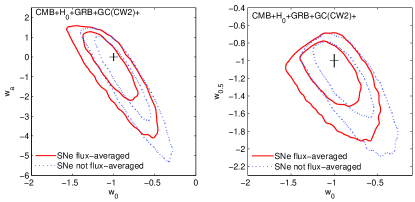
Fig.2 shows the 2D marginalized contours of (w0,wa)subscript𝑀0subscriptπ‘€π‘Ž(w_{0},w_{a}) and (w0,w0.5)subscript𝑀0subscript𝑀0.5(w_{0},w_{0.5}) for SNe data combined with with CMB, H0subscript𝐻0H_{0}, GRB, and GC (CW2) data. The solid contours are for flux-averaged SNe, and dotted contours are for SNe without flux-averaging. The SNe data with or without flux-averaging lead to qualitatively consistent results, with flux-averaging expanding the parameter space at w0<βˆ’1subscript𝑀01w_{0}<-1, which shifts the bestfit model from w0>βˆ’1subscript𝑀01w_{0}>-1 towards w0=βˆ’1subscript𝑀01w_{0}=-1, and from wa<0subscriptπ‘€π‘Ž0w_{a}<0 towards wa=0subscriptπ‘€π‘Ž0w_{a}=0 (it has a smaller impact on w0.5subscript𝑀0.5w_{0.5} since w0.5subscript𝑀0.5w_{0.5} is less correlated with w0subscript𝑀0w_{0} than wasubscriptπ‘€π‘Žw_{a}). Table 1 tabulates the mean and 68.3% confidence intervals for (w0,wa)subscript𝑀0subscriptπ‘€π‘Ž(w_{0},w_{a}) and (w0,w0.5)subscript𝑀0subscript𝑀0.5(w_{0},w_{0.5}) for SNe data combined with with CMB, H0subscript𝐻0H_{0}, GRB, with or without GC (CW2) data (the latter corresponds to Fig.2).

Table 1: Effect of flux-averaging SNe on (w0,wa)subscript𝑀0subscriptπ‘€π‘Ž(w_{0},w_{a}) and (w0,w0.5)subscript𝑀0subscript𝑀0.5(w_{0},w_{0.5})
flux-averaging w0subscript𝑀0w_{0} wasubscriptπ‘€π‘Žw_{a} w0subscript𝑀0w_{0} w0.5subscript𝑀0.5w_{0.5}
SNe+CMB+H0subscript𝐻0H_{0}+GRB
yes βˆ’0.9870.987-0.987 (βˆ’1.247,βˆ’0.7271.2470.727-1.247,-0.727) βˆ’0.7800.780-0.780 (βˆ’2.046,0.5162.0460.516-2.046,0.516) βˆ’0.9970.997-0.997 (βˆ’1.268,βˆ’0.7221.2680.722-1.268,-0.722) βˆ’1.2601.260-1.260 (βˆ’1.546,βˆ’0.9651.5460.965-1.546,-0.965)
no βˆ’0.7800.780-0.780 (βˆ’1.013,βˆ’0.5451.0130.545-1.013,-0.545) βˆ’1.4241.424-1.424 (βˆ’2.891,0.0452.8910.045-2.891,0.045) βˆ’0.7830.783-0.783 (βˆ’1.023,βˆ’0.5471.0230.547-1.023,-0.547) βˆ’1.2481.248-1.248 (βˆ’1.549,βˆ’0.9461.5490.946-1.549,-0.946)
SNe+CMB+H0subscript𝐻0H_{0}+GRB+GC(CW2)
yes βˆ’0.9950.995-0.995 (βˆ’1.211,βˆ’0.7761.2110.776-1.211,-0.776) βˆ’0.6760.676-0.676 (βˆ’1.884,0.566)-1.884,0.566) βˆ’1.0001.000-1.000 (βˆ’1.216,βˆ’0.784)-1.216,-0.784) βˆ’1.2111.211-1.211 (βˆ’1.454,βˆ’0.966)-1.454,-0.966)
no βˆ’0.8320.832-0.832 (βˆ’1.061,βˆ’0.606)-1.061,-0.606) βˆ’1.3531.353-1.353 (βˆ’2.844,0.151)-2.844,0.151) βˆ’0.8420.842-0.842 (βˆ’1.067,βˆ’0.615)-1.067,-0.615) βˆ’1.2661.266-1.266 (βˆ’1.559,βˆ’0.972)-1.559,-0.972)
Refer to caption
Figure 2: The 2D marginalized contours of (w0,wa)subscript𝑀0subscriptπ‘€π‘Ž(w_{0},w_{a}) and (w0,w0.5)subscript𝑀0subscript𝑀0.5(w_{0},w_{0.5}) for SNe data (with and without flux-averaging) combined with galaxy clustering (CW2), CMB, H0subscript𝐻0H_{0}, and GRB data. The contours are at 68% and 95% confidence levels.

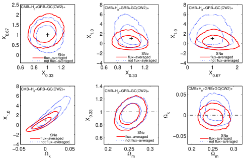
Fig.3 shows the 2D marginalized contours of (X0.33,X0.67,X1.0,Ξ©m,Ξ©k)subscript𝑋0.33subscript𝑋0.67subscript𝑋1.0subscriptΞ©π‘šsubscriptΞ©π‘˜(X_{0.33},X_{0.67},X_{1.0},\Omega_{m},\Omega_{k}) for SNe data combined with CMB, H0subscript𝐻0H_{0}, GRB, and GC data (CW2). The solid contours are for flux-averaged SNe, and dotted contours are for SNe without flux-averaging. The SNe data with or without flux-averaging lead to qualitatively consistent results, with a shift of the bestfit model towards a cosmological constant; this is the same trend as in the (w0,wa)subscript𝑀0subscriptπ‘€π‘Ž(w_{0},w_{a}) and (w0,w0.5)subscript𝑀0subscript𝑀0.5(w_{0},w_{0.5}) parametrizations. Note that flux-averaging leads to significantly tighter constraints on the dark energy density at z=1𝑧1z=1, X1.0subscript𝑋1.0X_{1.0}; this indicates that the impact of flux-averaging increases with redshift, since (X0.33,X0.67,X1.0)subscript𝑋0.33subscript𝑋0.67subscript𝑋1.0(X_{0.33},X_{0.67},X_{1.0}) are only weakly correlated. This is as expected, since the bias in estimated parameters due to weak lensing increases with redshift Wang (2005).
Refer to caption
Figure 3: The 2D marginalized contours of (X0.33,X0.67,X1.0,Ξ©m,Ξ©k)subscript𝑋0.33subscript𝑋0.67subscript𝑋1.0subscriptΞ©π‘šsubscriptΞ©π‘˜(X_{0.33},X_{0.67},X_{1.0},\Omega_{m},\Omega_{k}) for SNe data (with and without flux-averaging) combined with galaxy clustering (CW2), CMB, H0subscript𝐻0H_{0}, and GRB data. The contours are at 68% and 95% confidence levels.

III.2 Comparison of different galaxy clustering data

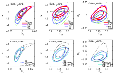
We now explore the differences of the various galaxy clustering (GC) measurements in constraining dark energy, assuming a constant equation of state for dark energy, w𝑀w. Fig.4 shows the 2D marginalized contours of (w,Ξ©m,Ξ©k)𝑀subscriptΞ©π‘šsubscriptΞ©π‘˜(w,\Omega_{m},\Omega_{k}) for different GC measurements combined with CMB, H0subscript𝐻0H_{0}, and GRB data.

The first row of Fig.4 compares the H​(z=0.35)​rs​(zd)𝐻𝑧0.35subscriptπ‘Ÿπ‘ subscript𝑧𝑑H(z=0.35)r_{s}(z_{d}) and rs​(zd)/DA​(z=0.35)subscriptπ‘Ÿπ‘ subscript𝑧𝑑subscript𝐷𝐴𝑧0.35r_{s}(z_{d})/D_{A}(z=0.35) measurements by Chuang & Wang (2011) CW11 with their d0.35=rs​(zd)/DV​(z=0.35)subscript𝑑0.35subscriptπ‘Ÿπ‘ subscript𝑧𝑑subscript𝐷𝑉𝑧0.35d_{0.35}=r_{s}(z_{d})/D_{V}(z=0.35) measurement (both from SDSS DR7 LRGs), as well as the d0.2subscript𝑑0.2d_{0.2} and d0.35subscript𝑑0.35d_{0.35} measurements by Percival et al. (2010) Percival10 from SDSS DR7 LRG and main galaxy samples and 2dFGRS, and the d0.6subscript𝑑0.6d_{0.6} measurement by Blake et al. (2011) from the WiggleZ survey Blake11 combined with the d0.106subscript𝑑0.106d_{0.106} measurement by Beutler et al. (2011) from 6dF GRS.

For the Chuang & Wang (2011) CW11 GC measurements (CW2 and CW1), the constraints on w𝑀w are tightened significantly by going from spherically-averaged data (CW1), i.e., d0.35subscript𝑑0.35d_{0.35}, to 2D data (CW2), i.e., H​(z=0.35)​rs​(zd)𝐻𝑧0.35subscriptπ‘Ÿπ‘ subscript𝑧𝑑H(z=0.35)r_{s}(z_{d}) and rs​(zd)/DA​(z=0.35)subscriptπ‘Ÿπ‘ subscript𝑧𝑑subscript𝐷𝐴𝑧0.35r_{s}(z_{d})/D_{A}(z=0.35), as indicated by comparing the thin solid contours (CW1) to thick solid contours (CW2) in the first row of Fig.4. This is as expected, as more information from GC is included in CW2 compared to CW1.

Both the Percival et al. (2010) GC measurements (WP) and the combined WiggleZ survey and 6dF GRS measurements (CB+) favor w<βˆ’1𝑀1w<-1, while the Chuang & Wang (2011) CW11 GC measurements favor w=βˆ’1𝑀1w=-1.

The second row in Fig.4 compares the d0.2subscript𝑑0.2d_{0.2} and d0.35subscript𝑑0.35d_{0.35} measurements by Percival et al. (2010) Percival10 (WP2), with their measurements of d0.2subscript𝑑0.2d_{0.2} and d0.35subscript𝑑0.35d_{0.35} separately. Clearly, most of the constraining power on w𝑀w comes from d0.35subscript𝑑0.35d_{0.35}. While the d0.2subscript𝑑0.2d_{0.2} measurement favors w=βˆ’1𝑀1w=-1, the d0.35subscript𝑑0.35d_{0.35} measurement favors w<βˆ’1𝑀1w<-1.

The measurements of d0.35subscript𝑑0.35d_{0.35} by Chuang & Wang (2011) CW11 and Percival et al. (2010) Percival10 are similar in precision, but differ systematically: d0.35C​W≑rs​(zd)/DV​(z=0.35)=0.1161Β±0.0034superscriptsubscript𝑑0.35πΆπ‘Šsubscriptπ‘Ÿπ‘ subscript𝑧𝑑subscript𝐷𝑉𝑧0.35plus-or-minus0.11610.0034d_{0.35}^{CW}\equiv r_{s}(z_{d})/D_{V}(z=0.35)=0.1161\pm 0.0034, while d0.35W​P≑rs​(zd)/DV​(z=0.35)=0.1097Β±0.0036superscriptsubscript𝑑0.35π‘Šπ‘ƒsubscriptπ‘Ÿπ‘ subscript𝑧𝑑subscript𝐷𝑉𝑧0.35plus-or-minus0.10970.0036d_{0.35}^{WP}\equiv r_{s}(z_{d})/D_{V}(z=0.35)=0.1097\pm 0.0036. The lower measured value of d0.35W​Psuperscriptsubscript𝑑0.35π‘Šπ‘ƒd_{0.35}^{WP} implies a smaller H​(z=0.35)𝐻𝑧0.35H(z=0.35), which in turn implies a more negative w𝑀w. When combined with CMB, H0subscript𝐻0H_{0}, and GRB data, d0.35C​Wsuperscriptsubscript𝑑0.35πΆπ‘Šd_{0.35}^{CW} favors w=βˆ’1𝑀1w=-1, while d0.35W​Psuperscriptsubscript𝑑0.35π‘Šπ‘ƒd_{0.35}^{WP} favors w<βˆ’1𝑀1w<-1. Note that these two measurements used different methods to analyze GC data: Chuang & Wang (2011) used the galaxy correlation function, while Percival et al. (2010) used galaxy power spectrum. It is not surprising that they lead to different distance measurements from GC.

For the rest of this paper, we will present only results using the GC measurements by Chuang & Wang (2011) CW11 ; these are more conservative as they were derived without assuming CMB priors.
Refer to caption
Figure 4: The 2D marginalized contours of (w,Ξ©m,Ξ©k)𝑀subscriptΞ©π‘šsubscriptΞ©π‘˜(w,\Omega_{m},\Omega_{k}) for different galaxy clustering measurements combined with CMB, H0subscript𝐻0H_{0}, and GRB data. The contours are at 68% and 95% confidence levels.

III.3 Constraints on dark energy and H​(z)𝐻𝑧H(z)

Figs.5-7 show the 2D marginalized contours of dark energy and cosmological parameters for the three different sets of dark energy parameters: (1) wX​(z)=wsubscript𝑀𝑋𝑧𝑀w_{X}(z)=w=const.; (2) wX​(z)=w0+wa​(1βˆ’a)subscript𝑀𝑋𝑧subscript𝑀0subscriptπ‘€π‘Ž1π‘Žw_{X}(z)=w_{0}+w_{a}(1-a), and wX​(z)=w0​(3​aβˆ’2)+3​w0.5​(1βˆ’a)subscript𝑀𝑋𝑧subscript𝑀03π‘Ž23subscript𝑀0.51π‘Žw_{X}(z)=w_{0}(3a-2)+3w_{0.5}(1-a); (3) X​(z)≑ρX​(z)/ρX​(0)𝑋𝑧subscriptπœŒπ‘‹π‘§subscriptπœŒπ‘‹0X(z)\equiv\rho_{X}(z)/\rho_{X}(0) given by a cubic spline at z<1𝑧1z<1 over Xzi≑X​(zi)subscript𝑋subscript𝑧𝑖𝑋subscript𝑧𝑖X_{z_{i}}\equiv X(z_{i}), with z1=1/3subscript𝑧113z_{1}=1/3, z2=2/3subscript𝑧223z_{2}=2/3, and z3=1subscript𝑧31z_{3}=1, and X​(z>1)=X​(z=1)𝑋𝑧1𝑋𝑧1X(z>1)=X(z=1).

Refer to caption
Figure 5: The 2D marginalized contours of (w,Ξ©m,Ξ©k)𝑀subscriptΞ©π‘šsubscriptΞ©π‘˜(w,\Omega_{m},\Omega_{k}) for SNe data (flux-averaged), galaxy clustering measurements (CW2), combined with CMB, H0subscript𝐻0H_{0}, and GRB data. The contours are at 68% and 95% confidence levels.
Refer to caption
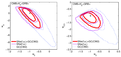
Figure 6: The 2D marginalized contours of (w0,wa)subscript𝑀0subscriptπ‘€π‘Ž(w_{0},w_{a}) and (w0,w0.5)subscript𝑀0subscript𝑀0.5(w_{0},w_{0.5}) for SNe data (flux-averaged), galaxy clustering measurements (CW2), combined with CMB, H0subscript𝐻0H_{0}, and GRB data. The contours are at 68% and 95% confidence levels.
Refer to caption
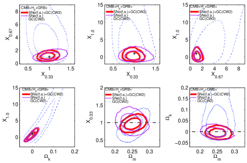
Figure 7: The 2D marginalized contours of (X0.33,X0.67,X1.0,Ξ©m,Ξ©k)subscript𝑋0.33subscript𝑋0.67subscript𝑋1.0subscriptΞ©π‘šsubscriptΞ©π‘˜(X_{0.33},X_{0.67},X_{1.0},\Omega_{m},\Omega_{k}) for SNe data (flux-averaged), galaxy clustering measurements (CW2), combined with CMB, H0subscript𝐻0H_{0}, and GRB data. The contours are at 68% and 95% confidence levels.

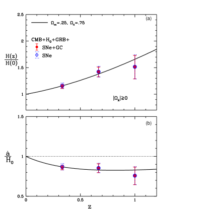
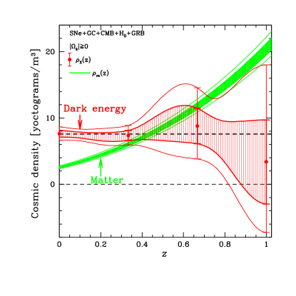
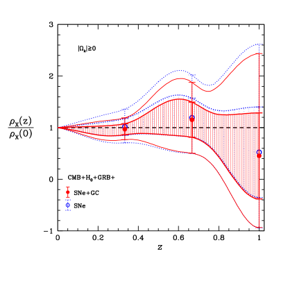
Fig.8 shows the dark energy density function ρX​(z)subscriptπœŒπ‘‹π‘§\rho_{X}(z) measured from SNe data (flux-averaged with d​z=0.07𝑑𝑧0.07dz=0.07), galaxy clustering measurements (CW2), combined with CMB, H0subscript𝐻0H_{0}, and GRB data. The upper panel of Fig.8 shows both ρX​(z)subscriptπœŒπ‘‹π‘§\rho_{X}(z) and ρm​(z)subscriptπœŒπ‘šπ‘§\rho_{m}(z), in units of yoctograms per cubic meter, with 1 yoctogram =10βˆ’24absentsuperscript1024=10^{-24} grams. The uncertainties in X​(z)𝑋𝑧X(z), Ξ©X=1βˆ’Ξ©mβˆ’Ξ©ksubscriptΩ𝑋1subscriptΞ©π‘šsubscriptΞ©π‘˜\Omega_{X}=1-\Omega_{m}-\Omega_{k}, and hβ„Žh have been propagated into that of ρX​(z)subscriptπœŒπ‘‹π‘§\rho_{X}(z). The lower panel of Fig.8 shows the corresponding X​(z)=ρX​(z)/ρX​(0)𝑋𝑧subscriptπœŒπ‘‹π‘§subscriptπœŒπ‘‹0X(z)=\rho_{X}(z)/\rho_{X}(0). Fig.9 shows the corresponding cosmic expansion history H​(z)𝐻𝑧H(z).

Clearly, given the same priors of CMB, H0subscript𝐻0H_{0}, and GRB data, SNe lead to much stronger constraints on dark energy than galaxy clustering data at present. Note also that the addition of galaxy clustering data to SN data leads to significantly improved constraints.
Refer to caption
Refer to caption
Figure 8: Dark energy density function ρX​(z)subscriptπœŒπ‘‹π‘§\rho_{X}(z) measured from SNe data (flux-averaged with d​z=0.07𝑑𝑧0.07dz=0.07), galaxy clustering measurements (CW2), combined with CMB, H0subscript𝐻0H_{0}, and GRB data. The contours are at 68% and 95% confidence levels. The upper panel shows both ρX​(z)subscriptπœŒπ‘‹π‘§\rho_{X}(z) and ρm​(z)subscriptπœŒπ‘šπ‘§\rho_{m}(z) in units of yoctograms per cubic meter, with 1 yoctogram =10βˆ’24absentsuperscript1024=10^{-24} grams. The lower panel shows the corresponding X​(z)=ρX​(z)/ρX​(0)𝑋𝑧subscriptπœŒπ‘‹π‘§subscriptπœŒπ‘‹0X(z)=\rho_{X}(z)/\rho_{X}(0).
Refer to caption
Figure 9: The cosmic expansion history H​(z)𝐻𝑧H(z) measured from SNe data (flux-averaged with d​z=0.07𝑑𝑧0.07dz=0.07), galaxy clustering measurements (CW2), combined with CMB, H0subscript𝐻0H_{0}, and GRB data. The error bars indicate the 68.3% confidence level ranges.

Table 2 gives the dark energy density function X​(z)≑ρX​(z)/ρX​(0)𝑋𝑧subscriptπœŒπ‘‹π‘§subscriptπœŒπ‘‹0X(z)\equiv\rho_{X}(z)/\rho_{X}(0) and the cosmic expansion history H​(z)𝐻𝑧H(z), as well as (Ξ©m,Ξ©k,h,Ο‰b)\Omega_{m},\Omega_{k},h,\omega_{b}), measured from current data of SNe+GC+CMB+H0subscript𝐻0H_{0}+GRB. The H​(z)𝐻𝑧H(z) measurements are derived using Eq.(II). Tables 3-4 give the normalized covariance matrices of the X​(z)𝑋𝑧X(z) and H​(z)𝐻𝑧H(z) measurements. Note that both the X​(z)𝑋𝑧X(z) and H​(z)𝐻𝑧H(z) measurements are only weakly correlated at different redshifts.

Table 2: X​(z)𝑋𝑧X(z), H​(z)𝐻𝑧H(z), and cosmological parameters estimated from current data with 68.3% C.L. upper and lower uncertainties.
ΞΌπœ‡\mu ΟƒπœŽ\sigma ΞΌ+Οƒβˆ’πœ‡superscript𝜎\mu+\sigma^{-} ΞΌβˆ’Οƒ+πœ‡superscript𝜎\mu-\sigma^{+}
X​(z=1/3)𝑋𝑧13X(z=1/3) 0.969 0.108 0.862 1.077
X​(z=2/3)𝑋𝑧23X(z=2/3) 1.152 0.347 0.812 1.492
X​(z=1.0)𝑋𝑧1.0X(z=1.0) 0.453 0.863 βˆ’0.3850.385-0.385 1.284
Ξ©msubscriptΞ©π‘š\Omega_{m} 0.252 0.016 0.236 0.268
Ξ©ksubscriptΞ©π‘˜\Omega_{k} βˆ’0.00490.0049-0.0049 0.0131 βˆ’0.01800.0180-0.0180 0.0080
hβ„Žh 0.734 0.019 0.715 0.753
Ο‰bsubscriptπœ”π‘\omega_{b} 0.02234 0.00062 0.02170 0.02290
H​(z=1/3)/H0𝐻𝑧13subscript𝐻0H(z=1/3)/H_{0} 1.148 0.040 1.107 1.186
H​(z=2/3)/H0𝐻𝑧23subscript𝐻0H(z=2/3)/H_{0} 1.419 0.093 1.328 1.510
H​(z=1.0)/H0𝐻𝑧1.0subscript𝐻0H(z=1.0)/H_{0} 1.511 0.221 1.289 1.731
Table 3: Normalized covariance matrix of X​(z)𝑋𝑧X(z) from current data
1 2 3
1 1.0000 0.1830 βˆ’0.11950.1195-0.1195
2 0.1830 1.0000 βˆ’0.12830.1283-0.1283
3 βˆ’0.11950.1195-0.1195 βˆ’0.12830.1283-0.1283 1.0000
Table 4: Normalized covariance matrix of H​(z)/H0𝐻𝑧subscript𝐻0H(z)/H_{0} from current data
1 2 3
1 1.0000 0.2657 0.0727
2 0.2657 1.0000 βˆ’0.05750.0575-0.0575
3 0.0727 βˆ’0.05750.0575-0.0575 1.0000

To quantify the comparison in dark energy constraints, we can use the general dark energy Figure-of-Merit (FoM) defined by Wang (2008b) Wang08b

FoM=1detCov​(f1,f2,…,fN)FoM1detCovsubscript𝑓1subscript𝑓2…subscript𝑓𝑁{\rm FoM}=\frac{1}{\sqrt{{\rm detCov}(f_{1},f_{2},...,f_{N})}} (44)

where (f1,f2,…,fN)subscript𝑓1subscript𝑓2…subscript𝑓𝑁(f_{1},f_{2},...,f_{N}) is the set of parameters that have been chosen to parametrize dark energy. The Dark Energy Task Force (DETF) defined the dark energy FoM to be the inverse of the area enclosed by the 95% confidence level contour of (w0,wa)subscript𝑀0subscriptπ‘€π‘Ž(w_{0},w_{a}) deft (2006). The areas enclosed by contours are difficult to calculate for real data, as these contours can be quite irregular. The definition of Eq.(44) has the advantage of being easy to calculate for either real or simulated data. For (f1,f2)=(w0,wa)subscript𝑓1subscript𝑓2subscript𝑀0subscriptπ‘€π‘Ž(f_{1},f_{2})=(w_{0},w_{a}), FoMFoM{\rm FoM} of Eq.(44) is proportional to the FoM defined by the DETF for ideal Gaussian-distributed data, and the same as the relative FoM used by the DETF in Fisher matrix forecasts.

Table 5 shows the dark energy FoM from SNe (flux-averaged), galaxy clustering measurements (CW2), together with CMB, H0subscript𝐻0H_{0}, and GRB data, for (w0,wa)subscript𝑀0subscriptπ‘€π‘Ž(w_{0},w_{a}), (w0,w0.5)subscript𝑀0subscript𝑀0.5(w_{0},w_{0.5}), and (X0.33,X0.67,X1.0)subscript𝑋0.33subscript𝑋0.67subscript𝑋1.0(X_{0.33},X_{0.67},X_{1.0}).

Table 5: Dark energy FoM from current data
CMB+H0subscript𝐻0H_{0}+GRB+ FoM({Xi})r{}_{r}(\{X_{i}\}) σ​(w0)𝜎subscript𝑀0\sigma(w_{0}) σ​(w0.5)𝜎subscript𝑀0.5\sigma(w_{0.5}) rw0,w0.5subscriptπ‘Ÿsubscript𝑀0subscript𝑀0.5r_{w_{0},w_{0.5}} FoM(w0,w0.5)r{}_{r}(w_{0},w_{0.5}) σ​(w0)𝜎subscript𝑀0\sigma(w_{0}) σ​(wa)𝜎subscriptπ‘€π‘Ž\sigma(w_{a}) rw0,wasubscriptπ‘Ÿsubscript𝑀0subscriptπ‘€π‘Žr_{w_{0},w_{a}} FoM(w0,wa)r{}_{r}(w_{0},w_{a})
SNe 18.61 0.27 0.33 βˆ’0.120.12-0.12 11.02 0.27 1.32 βˆ’0.700.70-0.70 3.98
GC 0.44 0.44 0.59 βˆ’0.740.74-0.74 5.76 0.39 2.40 βˆ’0.890.89-0.89 2.31
SNe+GC 32.00 0.22 0.27 βˆ’0.510.51-0.51 19.80 0.22 1.24 βˆ’0.840.84-0.84 6.74

IV Summary and Discussion

We have examined how dark energy constraints from current observational data depend on the analysis methods used: the analysis of Type Ia supernovae (SNe Ia), and that of galaxy clustering data (GC).

We generalize the flux-averaging analysis method of SNe Ia to allow correlated errors of SNe Ia, in order to reduce the systematic bias due to weak lensing of SNe Ia. We find that flux-averaging leads to larger errors on dark energy and cosmological parameters if only SN Ia data are used (see Fig.1). When SN Ia data (the latest compilation by the SNLS team) are combined with WMAP 7 year results, the latest Hubble constant (H0subscript𝐻0H_{0}) measurement using the HST, and gamma ray burst (GRB) data, flux-averaging of SNe Ia increases the concordance of SNe Ia with other data, and shifts the bestfit cosmological model notably closer to w=βˆ’1𝑀1w=-1 (see Fig.2 and Table 1). This leads to significantly tighter constraints on the dark energy density at z=1𝑧1z=1, and the cosmic curvature Ξ©ksubscriptΞ©π‘˜\Omega_{k} (see Fig.3). We have made our SN flux-averaging code publicly available at http://www.nhn.ou.edu/∼similar-to\simwang/SNcode/.

Note that since the flux-averaging of SNe Ia increases the concordance of SN Ia with other data, the combined data with flux-averaging of SNe Ia gives comparable constraints for most parameters, and smaller uncertainties for dark energy density at z=1𝑧1z=1, X1.0subscript𝑋1.0X_{1.0} (most affected by weak lensing), and Ξ©ksubscriptΞ©π‘˜\Omega_{k} (strongly correlated with X1.0subscript𝑋1.0X_{1.0}), compared with combined data with no flux-averaging of SNe Ia. The combination of concordant data tightens the overall constraints, while that of discordant data may not.

We find that given the same pirors (CMB+H0subscript𝐻0H_{0}+GRB), both the Percival et al. (2010) GC measurements Percival10 (WP: d0.2subscript𝑑0.2d_{0.2} and d0.35subscript𝑑0.35d_{0.35}) and the combined WiggleZ survey and 6dF GRS measurements Blake11 ; 6dF (CB+: d0.6subscript𝑑0.6d_{0.6} and d0.106subscript𝑑0.106d_{0.106}) favor w<βˆ’1𝑀1w<-1333Similar results were found by Esca11 ; XLi11 using Percival et al. (2010) GC measurements Percival10 ., while the Chuang & Wang (2011) GC measurements CW11 (CW2: H​(z=0.35)​rs​(zd)𝐻𝑧0.35subscriptπ‘Ÿπ‘ subscript𝑧𝑑H(z=0.35)r_{s}(z_{d}) and rs​(zd)/DA​(z=0.35)subscriptπ‘Ÿπ‘ subscript𝑧𝑑subscript𝐷𝐴𝑧0.35r_{s}(z_{d})/D_{A}(z=0.35)) favor w=βˆ’1𝑀1w=-1 (see Fig.4). This could be due to the difference in the analysis methods used to derive these GC measurements. We find that the GC measurements by Chuang & Wang (2011) are consistent with SN Ia data (which favor w=βˆ’1𝑀1w=-1), and tighten the dark energy constraints significantly when combined with SN data (see Fig.5-7).

For the convenience of future work, we have derived Gaussian fits to the probability distributions of a set of CMB parameters, [la​(zβˆ—),R​(zβˆ—),zβˆ—,ns,rs​(zd)subscriptπ‘™π‘Žsubscript𝑧𝑅subscript𝑧subscript𝑧subscript𝑛𝑠subscriptπ‘Ÿπ‘ subscript𝑧𝑑l_{a}(z_{*}),R(z_{*}),z_{*},n_{s},r_{s}(z_{d})], that summarize the WMAP7 data, as well as well their covariance matrix. Note that while [la​(zβˆ—),R​(zβˆ—),zβˆ—subscriptπ‘™π‘Žsubscript𝑧𝑅subscript𝑧subscript𝑧l_{a}(z_{*}),R(z_{*}),z_{*}] are sufficient for summarizing the CMB priors when nssubscript𝑛𝑠n_{s} dependence has been marginalized over in GC analysis, [la​(zβˆ—),R​(zβˆ—),zβˆ—,nssubscriptπ‘™π‘Žsubscript𝑧𝑅subscript𝑧subscript𝑧subscript𝑛𝑠l_{a}(z_{*}),R(z_{*}),z_{*},n_{s}] need to be used when the constraints on nssubscript𝑛𝑠n_{s} from GC are included (as will be the case for future GC data). We find that rs​(zd)subscriptπ‘Ÿπ‘ subscript𝑧𝑑r_{s}(z_{d}) gives redundant information, its measurement cannot be used in the CMB priors unless it is used to replace la​(zβˆ—)subscriptπ‘™π‘Žsubscript𝑧l_{a}(z_{*}). Also, our Gaussian fit for the pdf of rs​(zd)subscriptπ‘Ÿπ‘ subscript𝑧𝑑r_{s}(z_{d}) from WMAP7 can be useful when fitting for BAO peaks in GC data analysis.

We find that current data are fully consistent with a cosmological constant and a flat universe, consistent with the latest findings by others (see, e.g., Komatsu et al. (2011); XLi11 ; Bean10 ; Chen11 ; Dossett11 ; Holsclaw11 ; Liang11 ; SWang11 ). Since the uncertainties remain large, a deviation from a cosmological constant is far from being ruled out (see Fig.8).

At present, SN data provide much stronger constraints than GC data (see Table 5). This will change when ambitious galaxy surveys are carried out from space in the future Cimatti09 ; Wang10b . We can expect dramatic progress in our measurement and understanding of dark energy in the next decade or so.


Acknowledgements We are grateful to Alex Conley for communicating details of the SNLS data, to Eiichiro Komatsu for making the covariance matrix for [la​(zβˆ—),R​(zβˆ—),zβˆ—,rs​(zd),nssubscriptπ‘™π‘Žsubscript𝑧𝑅subscript𝑧subscript𝑧subscriptπ‘Ÿπ‘ subscript𝑧𝑑subscript𝑛𝑠l_{a}(z_{*}),R(z_{*}),z_{*},r_{s}(z_{d}),n_{s}] he derived from WMAP 7 year data available, and to Max Tegmark for suggesting the presentation of ρX​(z)subscriptπœŒπ‘‹π‘§\rho_{X}(z) in the upper panel of Fig.8. We acknowledge the use of CAMB and CosmoMC. YW and CHC are supported in part by DOE grant DE-FG02-04ER41305. PM is supported in part by the L’Oreal UK and Ireland Fellowship For Women in Science, and by the University of Sussex.

References

  • Riess et al.Β  (1998) Riess, A. G, et al., 1998, Astron. J., 116, 1009
  • Perlmutter et al.Β  (1999) Perlmutter, S. et al., 1999, ApJ, 517, 565
  • (3) Copeland, E.Β J., Sami, M., Tsujikawa, S., IJMPD, 15 (2006), 1753
  • (4) Ruiz-Lapuente, P., Class. Quantum. Grav., 24 (2007), 91
  • (5) Ratra, B., Vogeley, M.Β S., arXiv:0706.1565 (2007)
  • (6) Frieman, J., Turner, M., Huterer, D., ARAA, 46, 385 (2008)
  • (7) Caldwell, R. R., & Kamionkowski, M., arXiv:0903.0866
  • (8) Uzan, J.-P., arXiv:0908.2243
  • (9) Wang, Y., Dark Energy, Wiley-VCH (2010)
  • (10) Li, M., et al., 2011, arXiv1103.5870
  • Blake & Glazebrook (2003) Blake, C.; Glazebrook, K., 2003, ApJ, 594, 665
  • Seo & Eisenstein (2003) Seo, H; Eisenstein, D J 2003, ApJ, 598, 720
  • Hu (2002) Hu, W., 2002, PRD, 66, 083515
  • Jain & Taylor (2003) Jain, B. & Taylor, A. PRL, 91, 141302 (2003)
  • (15) Amati, L., et al. 2002, A&A, 390, 81
  • Bloom, Frail, & Kulkarni (2003) Bloom, J. S., Frail, D. A., & Kulkarni, S. R. 2003, ApJ, 594, 674
  • (17) Schaefer, B. E., 2003, ApJ, 583, L71
  • Komatsu et al. (2011) Komatsu, E., et al. 2011, Astrophys.J.Suppl., 192, 18
  • Riess et al.Β  (2011) Riess, A. G, et al., 2011, ApJ, 730, 119
  • Wang (2008a) Wang, Y., Journal of Cosmology and Astroparticle Physics, 05, 021 (2008).
  • Simpson & Peacock (2010) Simpson, F., & Peacock, J.A. 2010, Phys Rev D, 81, 043512
  • (22) Conley, A., et al., 2011, Astrophys.J.Suppl., 192, 1
  • (23) Hui, L., & Greene, P.B., PRD, 73, 123526 (2006)
  • (24) Clarkson, C., et al., arXiv:1109.2484v2
  • Wang (2000) Wang, Y., ApJ 536, 531 (2000)
  • Wang & Mukherjee (2004) Wang, Y., & Mukherjee, P. 2004, ApJ, 606, 654
  • Wang (2005) Wang, Y., JCAP, 03, 005 (2005)
  • (28) Chuang, C.-H.; and Wang, Y., arXiv:1102.2251
  • (29) Percival, W.J., et al. 2010, MNRAS, 401, 2148
  • (30) Blake, C., et al. 2011, MNRAS, 415, 2892
  • (31) Beutler, F., et al., 2011, arXiv:1106.3366, MNRAS, in press
  • Page (2003) Page, L., et al. 2003, ApJS, 148, 233
  • Wang & Mukherjee (2007) Wang, Y., & Mukherjee, P., PRD, 76, 103533 (2007)
  • (34) Li, H., et al., ApJ, 683, L1 (2008)
  • (35) Wang, Y., 2008b, Phys. Rev. D 77, 123525
  • Hu & Sugiyama (1996) Hu, W., & Sugiyama, N. 1996, ApJ, 471, 542
  • Eisenstein & Hu (1998) Eisenstein, D. & Hu, W. 1998, ApJ, 496, 605
  • Chev01 (2001) Chevallier, M., & Polarski, D. 2001, Int. J. Mod. Phys. D10, 213
  • (39) Komatsu, E., β€œwmap-prior-for-bao.pdf” at http://gyudon.as.utexas.edu/∼similar-to\simkomatsu/wmap7/
  • (40) Wang, Y., PRD, 80, 123525 (2009)
  • (41) Wang, Y., 2008b, PRD, 78, 123532
  • (42) Schaefer, B. E., 2007, ApJ, 660, 16
  • (43) Butler, N.R. et al., ApJ, 2007, 671, 656
  • (44) Butler, N.R. et al., ApJ, 2009, 694, 76
  • (45) Petrosian, V.; Bouvier, A.; Ryde, F., arXiv:0909.5051
  • (46) Shahmoradi, A., & Nemiroff, R.J., MNRAS, 2011, 411, 1843
  • Wang & Garnavich (2001) Wang, Y., and Garnavich, P. 2001, ApJ, 552, 445
  • Wang & Tegmark (2004) Wang, Y., & Tegmark, M. 2004, Phys. Rev. Lett., 92, 241302
  • Wang & Freese (2006) Wang, Y., & Freese, K. 2006, Phys.Lett. B632, 449 (astro-ph/0402208)
  • Linde (1987) Linde, A. D., β€œInflation And Quantum Cosmology,” in Three hundred years of gravitation, (Eds.: Hawking, S.W. and Israel, W., Cambridge Univ. Press, 1987), 604-630.
  • (51) Wang, Y.; Kratochvil, J. M.; Linde, A.; & Shmakova, M., JCAP 0412 (2004) 006
  • Lewis02 (2002) Lewis, A., & Bridle, S. 2002, PRD, 66, 103511
  • deft (2006) Albrecht, A.; Bernstein, G.; Cahn, R.; Freedman, W. L.; Hewitt, J.; Hu, W.; Huth, J.; Kamionkowski, M.; Kolb, E.W.; Knox, L.; Mather, J.C.; Staggs, S.; Suntzeff, N.B., Report of the Dark Energy Task Force, astro-ph/0609591
  • (54) Escamilla-Rivera, C.; et al., 2011, JCAP, 09, 003
  • (55) Li, X.-D., et al., JCAP 07 (2011) 011
  • (56) Bean, R.; Tangmatitham, M., PRD, 81, 083534
  • (57) Chen, Y.; Ratra, B., arXiv:1106.4294
  • (58) Dossett, J.N.; Moldenhauer, J.; Ishak, M., 2011, PRD, 84, 023012
  • (59) Holsclaw, T.; et al., arXiv:1104.2041
  • (60) Liang, N.; Wu, P.-X.; Zhu, Z.-H., 2011, RAA, 11, 1019
  • (61) Wang, S.; Li, X.-D.; Li, M., 2011, PRD, 83, 023010
  • (62) Cimatti, A., et al., Experimental Astronomy, 23, 39 (2009)
  • (63) Wang, Y., et al., MNRAS, 409, 737 (2010)