Resolving the LSND anomaly by neutrino diffraction

Abstract

In the charged pion decay, a neutrino is produced in pair with a charged lepton and they have the same production rate. In this paper we show that neutrinos have their own space-time correlations in a wide area and are detected in a different manner from charged leptons, owing to extremely small mass. The neutrino flux reveals a unique interference effect in the form of diffraction of non-stationary waves. The diffraction component of the flux shows a slow position-dependence and leads to an electron neutrino at short base-line regions. The electron neutrino flux at short distances is attributed to the neutrino diffraction and the one at long distances is to the normal flavor oscillation. The former depends upon the average mass-squared $\bar{m}^{2}_{\nu}$ and the latter depends upon the mass-squared difference $\delta m^{2}_{\nu}$. The LSND and the two neutrino experiment (TWN) measure $\bar{m}^{2}_{\nu}$ and the other experiments measure $\delta m^{2}_{\nu}$. Hence they are consistent with each other. The neutrino diffraction would supply valuable information on the absolute neutrino mass.

I Neutrino diffraction and LSND.

Time evolution of a charged pion state is determined by the Schrödinger equation with the weak interaction Hamiltonian, and the state vector of a single pion at $t=0$ becomes a superposition of one pion state and a state composed of a charged lepton and a neutrino at $t=\text{T}$. A decay of the pion is studied normally with a transition amplitude at the infinite T of plane waves, i.e., asymptotic boundary conditions. This paper presents that T-dependent probabilities of the decay products give valuable informations, particularly on the neutrino, that are not found with the asymptotic values. Since the wave function describes a time dependent development of the neutrino, the wave function is used to compute the time-dependent probability, which reveals wave phenomena. These physical quantities have been unable to observe experimentally with high precision before due to low statistics, but they are becoming possible with high statistics data of the current experiments. We study the neutrino detection probability in a situation where the initial pion is prepared in a plane wave using an S-matrix of a finite time interval.

If the neutrino at a detector region is highly correlated, this wave is different from an isolated free wave and is not expressed by the plane wave of satisfying the asymptotic boundary condition of the S-matrix. In this region, expressing neutrinos with plane waves and studying their detection processes with the ordinary S-matrix LSZ ; Low , are not appropriate. An S-matrix of a finite time interval defined by the Møller operator at the finite time interval $\Omega_{\pm}(\text{T})$ as, $S[\text{T}]=\Omega_{-}^{\dagger}(\text{T})\Omega_{+}(\text{T})$, is appropriate to study the finite-size correction of the neutrino detection probability. Since wave packets decrease rapidly at large $|{\vec{x}}|$ and satisfy the asymptotic boundary conditions, the S-matrix of a finite time interval is expressed with the wave packets. One feature of the scattering of the finite time interval is that $S[\text{T}]$ does not commute with the free Hamiltonian $H_{0}$ but satisfies

$$[S[\text{T}],H_{0}]=i({\partial\over\partial\text{T}}\Omega_{-}(\text{T}))^{\dagger}\Omega_{+}(\text{T})-i\Omega_{-}(\text{T})^{\dagger}{\partial\over\partial\text{T}}\Omega_{+}(\text{T}),$$ (1)

thus the energy is not conserved by $S[\text{T}]$. Final states of having the different energy from that of the initial state contribute to the finite-size correction of the transition probability. Furthermore, the finite-size correction has a universal property and is computed rigorously.

We study the neutrino in the pion decay with $S[\text{T}]$, and find that the neutrino flux has a large finite-size correction of a form of a diffraction. We summarize our results first. The fluxes of the neutrino and charged lepton in pion decays are defined with their detection rates and are given at a macroscopic distance in the form

$$P=P_{normal}+P_{diff}(\text{T}),$$ (2)

where $P_{normal}$ agrees with a normal term calculated with the standard method and $P_{diff}(\text{T})$ is a diffraction term which is derived from the energy-nonconserving final states. The diffraction components for the neutrino, $P_{diff}^{(\nu)}(\text{T})$, and for the charged lepton, $P_{diff}^{l}$(T), are expressed by the masses $m_{{\nu}_{i}},m_{l}$ and the mixing matrix $U_{i,e}$, where $i$ is the mass eigenstate, in the form

$$P_{diff}^{(\nu)}(\text{T})=C\text{T}\sum_{i}\tilde{g}(\text{T},\omega_{\nu_{i}})|U_{i,e}|^{2},\,P_{diff}^{l}=C\text{T}\tilde{g}(\text{T},\omega_{l}),$$ (3)

where $C$ is a constant obtained later, $\omega=\frac{m^{2}}{2E}$, and $\tilde{g}(\text{T},\omega)=g(\text{T},\omega)-\tilde{g}(\infty,\omega)$, where

$$\text{T}g(\text{T},\omega)=-i\int_{0}^{\text{T}}dt_{1}dt_{2}\frac{\epsilon(\delta t)}{|\delta t|}e^{i{\omega}\delta t}.$$ (4)

$\tilde{g}(\text{T},\omega)$ is positive definite and decreases with a product $\text{T}\omega$. $\text{T}\omega_{l}$ becomes large and $\tilde{g}(\text{T},\omega_{l})$ vanishes at a macroscopic time for the charged leptons, but $\tilde{g}(\text{T},\omega_{\nu_{i}})$ becomes finite for the neutrinos. Hence $P_{diff}(\text{T})$ is finite in neutrinos and depends upon an average mass-squared $\bar{m}_{\nu}^{2}$. $P_{normal}$ is the normal term and includes flavor oscillations with the period determined by the mass-squared differences $\delta m_{\nu}^{2}$. For charged leptons the diffraction terms vanish and physical quantities are computed with the normal term.

Due to the small mass, relativistic invariance, and other features, the diffraction effect becomes observable in the neutrinos. The detection rates become different from their production rates at the macroscopic distances. Especially because the energy-momentum is not conserved in the diffraction component, the helicity suppression mechanism does not work and the electron neutrino is not suppressed compared to the muon neutrino in the near-detector region. This resolves the LSND anomaly excess-LSND and some previous experiments.

II Position-dependent detection probability: one specie.

Now we derive the diffraction term Ishikawa-Tobita-prl . To show this effect being distinct from a flavor oscillation, the formula for one specie of neutrino is studied first.

We suppose that a neutrino is observed through its incoherent interaction with one of nucleus. Then its detection amplitude in the pion decay process is expressed as, $T=\int d^{4}x\,\langle l,{\nu}|H_{w}(x)|\pi\rangle$. Here a pion is prepared at a time $\text{T}_{\pi}$, and a neutrino is detected at $\text{T}_{\nu}$, where the distance $c(\text{T}_{\nu}-\text{T}_{\pi})$ is macroscopic. A detected neutrino is expressed by a wave packet that represents the nucleon wave function in a nucleus that neutrinos interact. The neutrino wave packet Ishikawa-Shimomura ; Ishikawa-Tobita-ptp ; Ishikawa-Tobita is described by the central values of the momentum and coordinate, $(\text{T}_{\nu},\vec{\text{X}}_{\nu})$ and the width, $\sigma_{\nu}$ Kayser ; Giunti ; Nussinov ; Kiers ; Stodolsky ; Lipkin ; Asahara . They are expressed in the form $|\pi\rangle=|{\vec{p}}_{\pi},\text{T}_{\pi}\rangle,\ |l,\nu\rangle=|l,{\vec{p}}_{l};\nu,{\vec{p}}_{\nu},\vec{\text{X}}_{\nu},\text{T}_{\nu}\rangle.$ The amplitude $T$ is written with the hadronic $V-A$ current and Dirac spinors in the form

$$T=\int d^{4}xd{\vec{k}}_{\nu}\,N_{1}\langle 0|J_{V-A}^{\mu}(x)|\pi\rangle\bar{u}({\vec{p}}_{l})\gamma_{\mu}(1-\gamma_{5})\nu({\vec{k}}_{\nu})$$

$$\times e^{ip_{l}\cdot x+ik_{\nu}\cdot(x-\text{X}_{\nu})-\frac{\sigma_{\nu}}{2}({\vec{k}}_{\nu}-{\vec{p}}_{\nu})^{2}},$$ (5)

where $N_{1}=ig\left({\sigma_{\nu}/\pi}\right)^{\frac{4}{3}}\left({m_{l}m_{\nu}}/{E_{l}E_{\nu}}\right)^{\frac{1}{2}}$, and the time $t$ is integrated in the region $\text{T}_{\pi}\leq t$. ${\sigma_{\nu}}$ is the size of the neutrino wave packet and was estimated using the size of a nucleus. The Gaussian form of the wave packet is used for the sake of simplicity to obtain the finite-size correction in this paper. Its long-distance behavior is the same in general wave packets as was verified in Ishikawa-Tobita-prl . The muon momentum of ${p}_{\mu}\approx{p}_{\pi}-{p}_{\nu}$ and broad tail of ${p}_{\mu}\neq{p}_{\pi}-{p}_{\nu}$ contribute to this amplitude. The former component is the normal one and the latter one is a diffraction component which is shown to be computable rigorously using a light-cone singularity of relativistic invariant systems.

The neutrino momentum ${\vec{k}}_{\nu}$ is integrated easily in Eq. $(\ref{amplitude})$ and the coordinate representation of the neutrino wave is obtained, which shows the time evolution of the neutrino wave function in the backward direction. At $t=\text{T}_{\nu}$, the wave function agrees with the Gaussian function of the center $\vec{\text{X}}_{\nu}$ and at $t\leq\text{T}_{\nu}$ the position of the center is at ${\vec{v}}_{\nu}(t-\text{T}_{\nu})+\vec{\text{X}}_{\nu}$, which overlaps with the pion and muon wave functions.

Integrating the space coordinates, a Gaussian function of the momenta, which shows that the momenta are approximately conserved, are obtained. The time is integrated in the finite interval $\text{T}=\text{T}_{\nu}-\text{T}_{\pi}$ and the amplitude is proportional to the T-dependent term,

$${\sin\left[({E(p_{\mu})+E({p_{\nu}})-E(p_{\pi})-{\vec{v}}_{\nu}\cdot({\vec{p}}_{\nu}+{\vec{p}}_{\mu}-{\vec{p}}_{\pi})})\text{T}/2\right]\over E(p_{\mu})+E({p_{\nu}})-E(p_{\pi})-{\vec{v}}_{\nu}\cdot({\vec{p}}_{\nu}+{\vec{p}}_{\mu}-{\vec{p}}_{\pi})}.$$ (6)

The energy is modified by the ${\vec{v}}_{\nu}$ dependent term and particularly the neutrino energy and momentum are combined to the small value, $E({p_{\nu}})-{\vec{v}}_{\nu}\cdot{\vec{p}}_{\nu}={m_{\nu}^{2}\over E_{\nu}}$. Hence the muon energy can be larger than that of the energy-momentum conserved system and leads the large finite-size correction.

To compute the amplitude and probability of this component rigorously, we introduce a correlation function and write the probability, after the spin summations are made, in the form

$$\int\frac{d{\vec{p}}_{l}}{(2\pi)^{3}}\sum_{s_{1},s_{2}}|T|^{2}$$

$$=\frac{N_{2}}{E_{\nu}}\int d^{4}x_{1}d^{4}x_{2}e^{-\frac{1}{2\sigma_{\nu}}\sum_{i}({\vec{x}}_{i}-\vec{x}_{i}^{\,0})^{2}}\Delta_{\pi,l}(\delta x)e^{i\phi(\delta x)},$$ (7)

where $N_{2}=g^{2}\left({4\pi}/{\sigma_{\nu}}\right)^{\frac{3}{2}}V^{-1}$, $V$ is a normalization volume for the initial pion, $\vec{x}_{i}^{\,0}=\vec{\text{X}}_{\nu}+{\vec{v}}_{\nu}(t_{i}-\text{T}_{\nu})$, $\delta x=x_{1}-x_{2}$, $\phi(\delta x)=p_{\nu}\!\cdot\!\delta x$ and

$$\Delta_{\pi,l}(\delta x)={\frac{1}{(2\pi)^{3}}}\int{d{\vec{p}}_{l}\over E({\vec{p}}_{l})}(2p_{\pi}\cdot p_{\nu}p_{\pi}\cdot p_{l}-m_{\pi}^{2}p_{l}\cdot p_{\nu})$$

$$\times e^{-i(p_{\pi}-p_{l})\cdot\delta x}.$$ (8)

In this expression the momentum is integrated first, which is possible because the probability is finite and integration variables can be interchanged.

The waves of charged lepton at the ultra-violet energy regions cause a light-cone singularity. Changing the variable to $q=p_{\pi}-p_{l}$ and integrating the four dimensional $q$, we are able to extract the light-cone singularity $\delta(\delta x^{2})\epsilon(\delta t)$ Ishikawa-Tobita-prl ; Wilson-OPE easily. The integral from the region $q^{0}\leq 0$ leads $\delta(\delta x^{2})\epsilon(\delta t)$ and the terms written by Bessel functions, while that from $0\leq q^{0}\leq E_{\pi}$ leads the rapidly oscillating term . The light-cone singularity is real without oscillation and is extended to infinity and the others either oscillate or decrease rapidly. So this expression is useful to find the finite-size correction of the probability which is unable to obtain with standard calculations of plane waves. In the first region the energy is not conserved, and the integral vanishes at $\text{T}=\infty$ in fact. The second one, on the other hand, is that of conserving the energy and determines the quantities at $\text{T}=\infty$. This expression of writing the probability with the light-cone singularity converges and is valid in the kinematical region $2p_{\pi}\!\cdot\!p_{\nu}\leq\tilde{m}_{l}^{2}$, where $\tilde{m}_{l}^{2}=m_{\pi}^{2}-m_{l}^{2}$.

Substituting the expression of $\Delta_{\pi,l}(\delta x)$ into Eq. $(\ref{probability-correlation})$, we have the phase factor of the neutrino wave at the light-cone position ${\vec{x}}=c{\vec{n}}_{\nu}(t-\text{T}_{\nu})+\vec{\text{X}}_{\nu}$ in the form, $\phi=E_{\nu}(t-\text{T}_{\nu})-{\vec{p}}_{\nu}\!\cdot\!({\vec{x}}-\vec{\text{X}}_{\nu})=\frac{m_{\nu}^{2}}{2E_{\nu}}(t-\text{T}_{\nu})$ of a slow angular velocity. Next an integration on the coordinates, $\vec{x}_{1}$ and ${\vec{x}}_{2}$, and $t_{1}$ and $t_{2}$ in the finite $\text{T}=\text{T}_{\nu}-\text{T}_{\pi}$, leads the slowly decreasing term $\tilde{g}(\text{T},\omega)$ and the normal term $G_{0}$. $\tilde{g}(\text{T},\omega)$ is generated from the light-cone singularity and related term and at $\text{T}=\infty$, $\tilde{g}(\text{T},\omega_{\nu})$ vanishes. The normal term, $G_{0}$, is from the rest. Due to the rapid oscillation in $\delta t$, $G_{0}$ gets contribution from the microscopic $\delta t$ region and is constant in T. This term does not depend on $\sigma_{\nu}$ and agrees with the normal probability obtained with the standard method of using plane waves. In the region $2p_{\pi}\!\cdot\!p_{\nu}>{\tilde{m}_{l}^{2}}$, $\Delta_{\pi,l}(\delta x)$ does not have a light-cone singularity and the diffraction term exists only in the kinematical region $2p_{\pi}\!\cdot\!p_{\nu}\leq{\tilde{m}_{l}^{2}}$. This region depends upon the charged-lepton mass, hence the diffraction terms of all three mass eigenstates converge in the union of the kinematical regions of the three masses, $2p_{\pi}\!\cdot\!p_{\nu}\leq{\tilde{m}_{\mu}^{2}}$. The diffraction terms is applied in this region in this paper.

We compute the total probability next. From the integration of neutrino’s coordinates $\vec{\text{X}}_{\nu}$ the total volume $V$ is obtained and cancelled with the normalization of the initial pion state. The total probability, then, becomes sum of the normal term $G_{0}$ and the diffraction term $\tilde{g}(\text{T},\omega_{\nu})$,

$$P=N_{3}\int\frac{d^{3}p_{\nu}}{(2\pi)^{3}}\frac{p_{\pi}\!\cdot\!p_{\nu}(m_{\pi}^{2}-2p_{\pi}\!\cdot\!p_{\nu})}{E_{\nu}}\left[\tilde{g}(\text{T},\omega_{\nu})+G_{0}\right],$$ (9)

where $N_{3}=8\text{T}g^{2}\sigma_{\nu}$ and $\text{L}=c\text{T}$ is the length of the decay region. $P$ is the neutrino flux when it interacts with the physical state of finite size target of $\sigma_{\nu}$. At finite T, the flux has the diffraction component, which is caused by the superposition of waves and stable under the variation of the pion’s momentum. At $\text{T}\rightarrow\infty$, the diffraction term vanishes and the probability $P$ agrees with the value of the standard calculation using plane waves.

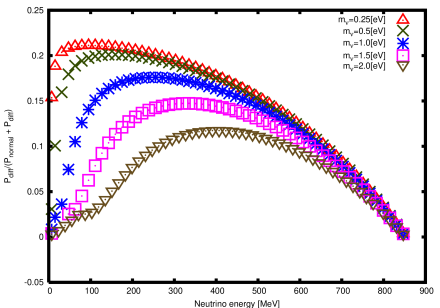
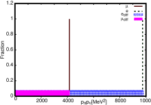
Figure 1: The neutrino energy and $p_{\pi}\cdot p_{\nu}$ dependences of the fraction of $P_{diff}$ are given in 1-a and 1-b. The horizontal axis shows $E_{\nu}$ in [MeV]. $m_{\nu}=0.25-2.0$ [eV/$c^{2}$], $E_{\pi}=2$ [GeV], and $\text{L}=50$ [m]. $p_{\pi}p_{\nu}$ dependence of the diffraction term is broad and that of the normal term is narrow.

Now we study each term in Eq. $(\ref{probability-3})$. In the normal term, energy and momentum are approximately conserved, and $G_{0}$ has a sharp peak at $p_{\pi}\!\cdot\!p_{\nu}={\tilde{m}_{l}^{2}/2}$. Hence the factor $m_{\pi}^{2}-2p_{\pi}\cdot p_{\nu}$ in Eq. $(\ref{probability-3})$ becomes $m_{l}^{2}$ and the rate is proportional to $m_{l}^{2}$. Integration of the neutrino’s angle leads this integral independent of the angle width, as far as it include the narrow peak. The value is independent also from $\sigma_{\nu}$, which is consistent with the condition for the stationary state Stodolsky , and agrees with the value of the ordinary method, which has the suppression of the electron mode. On the other hand, the diffraction component is present in the wide kinematical region, $|\vec{p}_{\nu}|(E_{\pi}-|\vec{p}_{\pi}|)\leq p_{\pi}\!\cdot\!p_{\nu}\leq{\tilde{m}_{l}^{2}/2}$ and depends on $\sigma_{\nu}$. The size of the nucleus of the mass number $A$, $\sigma_{\nu}=A^{\frac{2}{3}}/m_{\pi}^{2}$ makes the value, $\sigma_{\nu}=5.2/m_{\pi}^{2}$ for the ¹²C nucleus. Since the energy non-conserving states contribute, the diffraction component has a larger value of $m_{\pi}^{2}-2p_{\pi}\!\cdot\!p_{\nu}$ in Eq.$(\ref{probability-3})$ than $m_{l}^{2}$. Hence the branching ratio to the electron mode can become much larger than that of the normal terms and is determined by the integral of the diffraction component over the angle covered by the detector in the above region. This value is sensitive to the geometry of the experiment and could be much larger than $10^{-4}$, if the distance between the decay region and the detector is small.

The energy and $p_{\pi}\!\cdot\!p_{\nu}$ dependences of the fraction of the diffraction component are presented in Fig. 1 for $m_{\nu}=0.25-2\,[\text{eV}/c^{2}]$, ${E_{\pi}=2}$ [GeV], and $L=50$ [m]. The energy distribution of the diffraction term has a peak at ${E_{\nu}=100-200}$ [MeV], and the $p_{\pi}\!\cdot\!p_{\nu}$ distribution is broad in the diffraction component and is sharp in the normal component.

From Fig. $(\ref{fig:total-int-2})$, there is an excess due to the diffraction in the short distance region and the maximal excess is about $0.2$ of the normal term. The diffraction term is slowly varying with both the distance and energy. The typical length $\text{L}_{0}$ of this universal behavior is $\text{L}_{0}~{}[\text{m}]={2E_{\nu}\hbar c/m_{\nu}^{2}}=20\times{E_{\nu}[50\text{MeV}]/m_{\nu}^{2}[\text{eV}^{2}/c^{4}]}$. The diffraction is stable with the energy, hence a measurement with a finite uncertainty of the neutrino’s energy $\Delta E_{\nu}$, which is of the order $0.1\times E_{\nu}$, does not change the value much. For instance, with the uncertainty $5$ [MeV] of the energy $50$ [MeV] the diffraction component does not change at all. For a larger value of energy uncertainty, too, the diffraction is stable under a change of the energy and is computed from Eq. (9).

III Electron neutrino in pion decay.

Formulae for general three families are easily obtained from the one species formula. Since the light-cone singularity in $\Delta_{\pi,l}(\delta x)$ and the diffraction term have the universal form that is independent of the mass of the charged lepton, and depends upon the absolute neutrino mass, the diffraction term to the electron neutrino is obtained from the mixing matrix $U_{i,e}$, Eq. $(\ref{diffraction})$. Hence the flux of the electron neutrino is written with the average mass $\bar{m}_{\nu}^{2}$, $\sum_{i}\tilde{g}(\text{T},\omega_{\nu_{i}})|U_{i,e}|^{2}=\tilde{g}(\text{T},\bar{\omega}_{\nu}),\bar{\omega}_{\nu}={{\bar{m}_{\nu}}^{2}}/{2E_{\nu}}$. The average value coincides with $m_{{\nu}_{i}}$ if the $\delta m_{\nu}^{2}$ are much smaller than the average value.

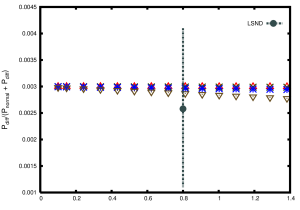
(a) LSND

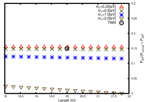
(b) TWN

Figure 2: The fraction of the diffraction probability at a finite distance L are given for LSND (2-a)and TWN (2-b). The horizontal axis shows the distance in [m] and the vertical axis shows fractions. The two values are very different but are consistent and agree with the diffraction predictions. $\bar{m}_{\nu}=0.25-2.0$ [eV/$c^{2}$], $P_{\pi}=350$ [MeV/$c$] in LSND and $300$ [MeV/$c$] in TWN, and $E_{\nu}=60$ [MeV] in LSND and $100$ [MeV] in TWN.

Historically using neutrinos in pion decays, TWN excess-two-neutrino proved that two neutrinos are different, and LSND excess-LSND claimed observation of $\nu_{\mu}\rightarrow\nu_{e}$ transition with a large $\delta m_{\nu}^{2}=0.1-1.0\,[\text{eV}^{2}/{c^{4}}]$. Unfortunately this value is inconsistent with MiniBooNE excess-MiniBoone which was designed to to test LSND and the values $\delta m_{\nu}^{2}=7.6\times 10^{-5},2.4\times 10^{-3}\,[\text{eV}^{2}/{c^{4}}]$ from other experiments particle-data . TWN found also signals of electron neutrino flux at an order of $10-20$ per cent, which is too large for the flavor oscillation assumption. So electron neutrino events of LSND and TWN are inconsistent with other neutrino experiments, if they are attributed to flavor oscillations. They have been puzzles for quite some time.

Now we compare the theoretical value of electron neutrino events with experiments. The normal component is negligibly small due to helicity suppression and the diffraction component $P_{diff}$ is finite and is studied. The neutrino flux in the decay pipe area is computed from the diffraction formula and the neutrino expressed by the wave packet of $\sigma_{\nu}$ determined by the detector propagates freely in the next area between the decay pipe and the detector region. The distribution is spread with $p_{\pi}\!\cdot\!p_{\nu}$ and has different geometrical behaviors from the normal component in the detector. Effects of geometries are important. The geometries of TWN and LSND are similar and the lengths between the pion source and the neutrino detector, $L_{d-s}$, and those of the decay region, $L_{d-reg}$, are given in Table 1.

Table 1: Geometries of experiments

Experiment	$L_{d-s}$	$L_{d-reg}$
TWN	30 [m]	20 [m]
LSND	30 [m]	0.7 [m]
CDHSW(N)	120 [m]	50 [m]
MiniBooNE	500 [m]	25 [m](diameter = 12.2 [m])
CDHSW(F)	600 [m]	50 [m]
KARMEN	-	Stopped pion or muon decay

Table 2: Experimental values and theoretical values

Experiment	$P_{\nu_{e}}/P_{\nu_{\mu}}$ (Exp)	$P_{diff}/P_{normal}$ (Th)
TWN	$0.18$	0.17
LSND	$(2.6\pm 1.0\pm 0.5)\times 10^{-3}$	$2.8\times 10^{-3}$
CDHSW(N)	?	0.2-0.5
CDHSW(F)	?	$0.02-0.05$
MiniBooNE, KARMEN	0	$\approx 10^{-5}$

$0.7\,[\text{m}]$ of $L_{d-reg}$ is the length of the decay region in air, while the whole decay region is $1.8\,[\text{m}]$. Since the length between the detectors and the sources of MiniBooNE and CDHSW(F) neutrino-CDHS is as large as 10 times those of TWN and LSND, the contributions of diffraction terms are $1\over 100$ of TWN and LSND. At CDHSW(N), the length is $4$ times of TWN and LSND but the energy is higher and about the same magnitude of the diffraction term is obtained. The diffraction term comes from the tree diagram and is suppressed strongly in matter, KARMEN neutrino-KARMEN . The diffraction component is important in decay in air but is complicated in decay in matter. Its magnitude will be studied in a future publication.

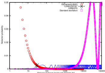
Figure 3: Electron neutrino flux of the neutrino diffraction is compared with flavor oscillations. The horizontal axis shows the distance in [m] and the vertical axis shows the fraction of the electron neutrino. The diffraction agrees with the LSND. The value from $\Delta m^{2}$ of the standard oscillation parameters becomes negligible at 30 M. To fit with the experiment by the flavor oscillation, a sterile neutrino of $\Delta m^{2}\approx 1(eV/c^{2})^{2}$ is necessary.

We compute the fraction of the diffraction components by taking into account the geometry. In LSND, the decay region in air is about $0.7\,[\text{m}]$ long and the detector is located $30\,[\text{m}]$ away from the decay region. In this case, the ratio becomes $0.28$ percent at $\bar{m}_{\nu}=1\,[\text{eV}/c^{2}]$. In TWN, the decay region is about $20\,[\text{m}]$ long and the detector is located $10\,[\text{m}]$ away from the decay region. The neutrino detection angle is much wider and the ratio becomes about $17$ percent at $\bar{m}_{\nu}=1\,[\text{eV}/c^{2}]$. In CDHSW, the energies of pion and neutrino are higher and iron is used for the detector. Including these effects, theoretical values are obtained.

The ratios $P_{diff}/P_{normal}$ of our theory and $P_{\nu_{e}}/P_{\nu_{\mu}}$ of experiments are summarized in Table 2. Uncertainties in TWN are not known and ignored. The fractions of the diffraction components obtained in this way are presented in Fig. 2 for the mass of the neutrino, $\bar{m}_{\nu}=0.25-2\,[\text{eV}/c^{2}]$, and the pion momentum ${p_{\pi}=350}$  [MeV/c] in LSND and ${300}$  [MeV/c] in TWN, and the neutrino energy $E_{\nu}=60$ [MeV] in LSND and $=100$ [MeV] in TWN. The fractions of the theory agree with those of the experiments using the same $\bar{m}_{\nu}$.

The magnitude of electron neutrino flux agreed with LSND in flight and TWN but not to others including MiniBooNE. Since matter effect in LSND at rest is complicated, we study only LSND in flight here. In Fig.3, the electron neutrino fraction from the neutrino diffraction is compared with those of the flavor oscillations of standard parameters of $\Delta m^{2}$ and of a sterile neutrino. The neutrino diffraction explains naturally the excess of the electron neutrino. Thus the puzzles are resolved and consistent understanding of the neutrino experiments are obtained. Furthermore, information on the absolute neutrino mass is obtained particle-data ; Tritium ; WMAP-neutrino .

IV Summary and implications.

It is found that the neutrino detection rate has the unusual finite-size correction in the macroscopic distance. Instead of the standard S-matrix $S[\infty]$, which is useless to study the finite-size correction, we studied the S-matrix of the finite time interval $S[\text{T}]$ and computed the finite-size correction of the detection probabilities which are measured in experiments. The asymptotic boundary conditions must be satisfied for the scattering or decay processes, hence the wave packets are necessary for $S[\text{T}]$ and are used. One feature is that S[T] does not commute with the free Hamiltonian $H_{0}$ and both final states of conserving the energy and those of non-conserving energy contribute. The rate from the former is independent of both T and $\sigma_{\nu}$ and agrees with that of the standard method, while that from the latter depends on T and $\sigma_{\nu}$ and does not satisfy various relations of the former such as the helicity suppression, symmetry between the neutrinos and charged leptons, and others.

The electron neutrino flux due to the diffraction was computed in the geometries of LSND and TWN and excellent agreements between the theory and experiments are obtained. Because the electron neutrino flux due to diffraction is determined by the average neutrino mass $\bar{m}_{\nu}$, the excesses of the electron neutrino suggest that $\bar{m}_{\nu}$ is around $0.25-1.0\,[\text{eV}/c^{2}]$. If the $\bar{m}_{\nu}$ is in this range and $\delta m^{2}_{\nu}$ of the experiments are used, LSND and TWN electron events are attributed to the diffraction component but not to the flavor oscillation. Thus the controversy related with LSND and TWN are resolved. Some information on the absolute neutrino mass is obtained, furthermore.

The confirmation of the neutrino diffraction would be made in a new experiment from the unique behaviors of the neutrino spectrum on the $p_{\pi}\!\cdot\!p_{\nu}$, energy, and angle. Since the helicity suppression does not work in the diffraction component, the flux of the electron neutrino becomes about $10-20$ % of that of the muon neutrino at the maximum value. Furthermore it has the unique properties that are very different from the normal term. If clear distinctions are observed on the dependences of these variables and agreements with the theory are found, the neutrino diffraction will be confirmed. Since at much larger distance than the above length, the diffraction component disappears and only the normal flavor oscillation terms remain, the experiment to measure the excess due to the diffraction component should be made at a short distance.

The present results may exhibit violations of two important relations, the unitarity and lepton number conservation. However that is not the case and they are not violated. First, from the behavior of the diffraction component that the detection rate is decreasing with T, the neutrino number looks decreasing and an unitarity is violated superficially. Since the neutrino is detected at the distant position, the detection time is delayed. The retarded and interference effects made the detection probability deviate from the neutrino number. Hence the decreasing behavior of $P({\text{T}})$ is in-connected with both the decreasing neutrino number and unitarity. In the text, $P({\text{T}})$ is computed with $S[\text{T}]$ that satisfies the proper boundary condition of the experiments and the unitarity condition $S[\text{T}]^{\dagger}S[\text{T}]=1$. If the T dependent neutrino probability were computed with $S[\infty]$, this would not have decreased with T. However, the $S[{\infty}]$ does not satisfy the proper boundary condition for the neutrino at T and is neither applied nor compared with the probability measured by the experiment. $S[\text{T}]$, on the other hand, satisfies the proper boundary condition and is used for comparisons with the experiments at the finite T. One of the important findings of the present work is that $S[\text{T}]$ gives the different results from $S[\infty]$ even in the macroscopic T. Second, asymmetric behaviors of $\tilde{g}(\text{T},\omega)$ lead that the neutrino detection rates are very different from those of the charged leptons. This is not in-consistent with the lepton number conservations but means that the detection probability is different from the neutrino number owing to the finite-size correction caused by retarded and interference effects. When either the neutrinos or the charged leptons are observed, their detection rates are different. Nevertheless, when both of neutrino and charged lepton are observed simultaneously, they have the same rates, due to the lepton number conservations.

The shorter life time of the pion in the situation when the neutrino is observed at a small distance than that of the free pion has not been tested and will be confirmed in a future experiment. Then if the muon is measured simultaneously, this muon shows the same behavior from the lepton number conservation. The detection rate of the muon depends on the boundary condition on the neutrino.

In this paper we ignored the higher order effects such as the pion life time and the pion mean free path in studying the quantum effects. We will study these problems, the muon decay, and other large scale physical phenomena of low energy neutrinos in subsequent papers.

References

- (1) H. Lehman, K. Symanzik, and W. Zimmermann, Nuovo Cimento. 1, 1425(1955).
- (2) F. Low, Phys. Rev. 97, 1392(1955).
- (3) C. Athanassopoulos, et al, Phys. Rev. Lett. 75, 2650-2653, (1995); .77, 3082-3085, (1996); 81, 1774-1777, (1998).
- (4) K. Ishikawa and Y. Tobita, arXiv:1106.4968[hep-ph]
- (5) K. Ishikawa and T.Shimomura, Prog. Theor. Phys. 114, (2005), 1201-1234. arXiv:hep-ph/0508303
- (6) K. Ishikawa and Y. Tobita, Prog. Theor. Phys. 122, (2009), 1111-1136. arXiv:0906.3938[quant-ph]
- (7) K. Ishikawa and Y. Tobita, arXiv:0801.3124; “Neutrino mass and mixing” in the 10th Inter. Symp. on “Origin of Matter and Evolution of Galaxies” AIP Conf. proc. 1016, P.329(2008)
- (8) B. Kayser, Phys. Rev. D24, 110(1981);
- (9) C. Giunti, C. W. Kim, and U. W. Lee, Phys. Rev. D44, 3635(1991)
- (10) S. Nussinov, Phys. Lett. B63, 201(1976)
- (11) K. Kiers, S. Nussinov and N. Weiss, Phys. Rev. D53, 537(1996).
- (12) L. Stodolsky, Phys. Rev. D58, 036006(1998).
- (13) H. J. Lipkin, Phys. Lett. B642, 366(2006).
- (14) A. Asahara, K. Ishikawa, T. Shimomura, and T. Yabuki, Prog. Theor. Phys. 113, 385(2005); T. Yabuki and K. Ishikawa, Prog. Theor. Phys. 108, 347(2002).
- (15) K. Wilson, in Proceedings of the Fifth International Symposium on Electron and Photon Interactions at High Energies, Ithaca, New York, 1971, p.115 (1971). See also N. N. Bogoliubov and D. V. Shirkov, Introduction to the Theory of Quantized Fields (John Wiley & Sons, Inc. New York, 1976).
- (16) G. Danby, et al, Phys. Rev. Lett. 9, 36-44, (1962).
- (17) A. A. Aguilar-Arevalo, et al, Phys. Rev. Lett.Vol. 102, 101802, (2009); ibid, 103, 111801, (2009) .
- (18) K. Nakamura et al. [Particle Data Group], J. Phys. G 37, 075021 (2010).
- (19) F. Dydak, et al, Phys. Lett. Vol. B134, 281, (1984).
- (20) B. E. Bodmann, et al, Phys. Lett. Vol. B332, 251, (1994). B. Armbruster, et al, Phys.Rev.C 57, 3414, (1998).
- (21) C. Weinheimer, et al. Phys. Lett. B460, 219–226 (1999).
- (22) E. Komatsu, et al. Astrophys. J. Suppl. 180, 330–376 (2009).