Internal Structure of Stellar Clusters:
Geometry of Star Formation

Abstract

The study of the internal structure of star clusters provides important clues concerning their formation mechanism and dynamical evolution. There are both observational and numerical evidences indicating that open clusters evolve from an initial clumpy structure, presumably a direct consequence of the formation in a fractal medium, toward a centrally condensed state. This simple picture has, however, several drawbacks. There can be very young clusters exhibiting radial patterns maybe reflecting the early effect of gravity on primordial gas. There can be also very evolved cluster showing fractal patterns that either have survived through time or have been generated subsequently by some (unknown) mechanism. Additionally, the fractal structure of some open clusters is much clumpier than the average structure of the interstellar medium in the Milky Way, although in principle a very similar structure should be expected. Here we summarize and discuss observational and numerical results concerning this subject.

1 Introduction

Most of visible matter in the universe is condensed into stars, with densities more than 30 orders of magnitude higher than the average density of the universe and more than 20 orders of magnitude higher than the densities of the interstellar clouds in which they form (Larson 2007). Thus, the fundamental question is not how baryons end up as stars, but how some of them form stars and others remain as hot, low-density interstellar gas. This enigma lies at the core of a predictive theory of star formation, one of the main goals of modern astronomy. We are still far away from a global solution to this complex problem, whose answer depends very much on the existence of a well-structured and complete set of empirical data, as well as on the building of reliable and precise simulation tools.

Nowadays, it is widely accepted that stars form in highly hierarchical stellar systems that mimic, in some way, the stepped structure of the interstellar medium (ISM) or, at least, the morphology of the densest regions. This hierarchical pattern, both spatial and temporal, presents singular condensations, the stellar clusters, whose main physical characteristics make them reliable tracers of the star forming processes in galaxies. Hierarchical structure extends from star complexes (or large portions of spiral arms in flocculent galaxies) through embedded clusters to individual young stars inside those embedded clusters. The cluster scale is the best metric to measure and analyze the whole spatial range in the formation of stellar systems.

The study of star forming regions in the infrared range led to the conclusion that most stars, if not all, born grouped in clusters (Lada & Lada 2003). However, after ten million years, the fraction of stars in clusters is reduced to 10% and this figure tends to decrease with age. This simple temporal pattern suggests that a few million years after their birth star clusters suffer a high mortality rate. The survivors evolve then under different destruction processes and are gradually eroded until diluted into the galactic field.

The initial conditions, that is, the properties of the cold and dark clouds that eventually form stars are poorly known (Bergin and Tafalla 2007). A few years ago, we started a project aimed to characterize the geometry of the ISM. This information would provide important clues on the physical processes developing and maintaining the internal structure of the clouds. Since the pioneering work by Larson (1981), turbulence is considered the best candidate to do this job. It appears that the distribution of gas and dust in these clouds determines the initial conditions of a newborn cluster because star formation follows the patterns defined by the densest regions (Bonnell et al. 2003). Thus, the fractal (self-similar) distribution of the gas in molecular cloud complexes may account for the hierarchical structure observed in some open clusters (Elmegreen 2010). However, observations show that the morphologies of young clusters show a wide variety, from hierarchical to centrally condensed ones, often being elongated or surrounded by a low-density stellar halo (see, for example, Maíz-Apellániz 2001; Hartmann 2002; and Caballero 2008). The reasons for this heterogeneity of shapes are still poorly understood.

Here we review and discuss the formation of star clusters and their evolution from a geometric point of view. In particular, our framework is determined by several questions: What do physical mechanisms control and shape the internal structure of fertile gas clouds? What is the influence of the geometric structure of a star-forming cloud on the internal spatial structure of the stellar population formed from it? How does it evolve with time? Because of the hierarchical and self-similar nature involved, fractal geometry appears to be a good descriptor for these physical structures. Thus, the design and development of mathematical tools for determining the fractal dimension of 3D gas clouds and point-like object distributions are also discussed and evaluated in this work.

2 Fractal dimension of the interstellar medium

Gas and dust in the Galaxy are organized into irregular structures in a hierarchical and approximately self-similar manner. This means that interstellar clouds can be well described or characterized as fractal structures (Mandelbrot 1983). Many tools can be used to characterize the complexity of these structures (see Elmegreen & Scalo 2004) but to measure the fractal dimension seems particularly appropriate when dealing with nearly fractal systems. The measurement of the dimension of the projected boundaries $D_{per}$ is the most used method to characterize the fractal properties of interstellar clouds, but there is a wide variation in the estimated values. A summary of results that can be accessed via NASA’s ADS service is shown in Table 1.

Table 1: Summary of perimeter dimensions in molecular clouds in the Galaxy

Ref.	$D_{per}$	Region/Map
(1)	$1.40$	Extinction maps of dark clouds
(2)	$1.12-1.40$	Dust emission maps of cirrus clouds
(3)	$1.17-1.30$	Infrared intensity and column density maps of several molecular clouds
(4)	$1.36$	Molecular emission maps (Taurus complex)
(5)	$1.38-1.52$	Visual extinction maps (Chamaeleon complex)
(6)	$1.51$	Molecular emission map (Taurus complex)
(7)	$1.23-1.54$	HI maps of high-velocity clouds and infrared maps of cirrus clouds
(8)	$1.34-1.40$	Molecular emission maps of clouds in the antigalactic center
(9)	$1.31-1.35$	Molecular emission maps (Ophiuchus, Perseus, and Orion clouds)
(10)	$1.50-1.53$	Molecular emission maps of clouds in the outer Galaxy

Reference index: (1) Beech (1987); (2) Bazell & Desert (1988); (3) Dickman et al. (1990); (4) Falgarone et al. (1991); (5) Hetem & Lepine (1993); (6) Stutzki (1993); (7) Vogelaar & Wakker (1994); (8) Lee (2004); (9) Sánchez et al. (2007a); (10) Lee et al. (2008).

In general, observed values are spread over the range $1.1\lesssim D_{per}\lesssim 1.5$. It is not clear, however, whether the different values seen in Table 1 represent real variations or they are consequence of different data quality and/or analysis techniques. For example, it is well known that the obtained results may be affected by factors such as image resolution and/or signal-to-noise ratio (Dickman et al. 1990; Vogelaar & Wakker 1994; Lee 2004; Sánchez et al. 2005, 2007a). Note, for example, that for CO emission maps of the same region in the Taurus molecular complex Falgarone et al. (1991) obtained $D_{per}=1.36$ whereas Stutzki (1993) found $D_{per}=1.51$ on a different set of data. Despite those results, the general “belief” is that the fractal dimension of the projected boundaries of interstellar clouds is roughly a constant throughout the Galaxy, with $D_{per}\simeq 1.3-1.4$ (Bergin & Tafalla 2007). This constancy in $D_{per}$ would be a natural consequence of a universal picture in which interstellar turbulence is driven by the same physical mechanisms everywhere (Elmegreen & Scalo 2004). In order to get reliable clues about the ISM structure, it is important that any analysis technique is applied systematically on homogeneous data sets. Sánchez et al. (2007a) used several maps of different regions (Ophiuchus, Perseus, and Orion molecular clouds) in different emission lines and calculated $D_{per}$ by using an algorithm previously calibrated on simulated fractals (Sánchez et al. 2005). In this case the range of obtained values decreased notoriously to $1.31\lesssim D_{per}\lesssim 1.35$ (reference $9$ in Table 1).

But what is the corresponding value of the fractal dimension of interstellar clouds in the three-dimensional space, $D_{f}$? It has been traditionally assumed that $D_{f}=D_{per}+1\simeq 2.3-2.4$ (Beech 1992). Sánchez et al. (2005) used simulated fractal clouds to study the relationship between $D_{per}$ and $D_{f}$ and showed this assumption is not correct. Their main result (see their Figure $8$) indicate that if the perimeter dimension is around $D_{per}\simeq 1.31-1.35$ (Sánchez et al. 2007a) then the 3D fractal dimension should be in the range $D_{f}\sim 2.6-2.8$. This dimension is clearly higher than the value $D_{f}\sim 2.3$ that is usually assumed in the literature for interstellar clouds in the Galaxy (Bergin & Tafalla 2007).

3 Fractal dimension of young stellar clusters

The distribution of stars and star-forming regions also exhibits a spatial hierarchy from large star complexes to individual clusters (Efremov 1995; de la Fuente Marcos & de la Fuente Marcos 2006, 2009; Elias et al. 2009; Elmegreen 2010). This hierarchical structure is presumably a direct consequence of the fact that stars are formed in a medium with an underlying fractal structure (previous Section). If this were the case, then it is reasonable to assume that the fractal dimension of the distribution of new-born stars should be nearly the same as that of the molecular clouds from which they are formed.

The fractal dimension of a distribution of stars can be measured by using the correlation integral $C(r)$. For a fractal set it holds that $C(r)\sim r^{D_{c}}$, being $D_{c}$ the so-called correlation dimension. Calculating the mean surface density of companions (MSDC) per star $\Sigma(\theta)$ as a function of angular separation $\theta$ is another widely used way to measure the degree of clustering of stars. For fractals $\Sigma(\theta)\sim\theta^{\gamma}$, and the exponent is related to the fractal dimension through $D_{c}=2+\gamma$. MSDC technique has been used by various authors to study the clustering of protostars, pre-main sequence stars, or young stars in different star-forming regions. Most results seem to indicate that there are two different ranges of spatial scales, the regime of binary and multiple systems on smaller scales and a regime of fractal clustering on the largest scales. The idea prevalent among astronomers is that self-similar clustering above the binary regime is due to, or arises from, the fractal features of the parent clouds. However, such as in the case of gas distribution in the ISM, if one checks the references a wide variety of different values can be found. Nakajima et al. (1998) found significantly variations among different star-forming regions with $1.2\lesssim D_{c}\lesssim 1.9$. There can be large differences even in the same regions if analyzed by different authors and data sets. For example, in the Taurus region both Larson (1995) and Simon (1997) analyzed young stars and their results are in perfect agreement with $D_{c}\simeq 1.4$, whereas Hartmann (2002) and Kraus & Hillenbrand (2008) both agree in $D_{c}\simeq 1.0$ for the same region. Table 2 summarizes the wide range of $D_{c}$ values estimated by using the MSDC technique. Obviously, there can be different results depending on data sources, object selection criteria, and details of the specific calculation procedures. But additionally, it has been shown that if boundary and/or small data-set effects are not taken into account the final results can be seriously biased, given fractal dimension values smaller than the true ones (Sánchez et al. 2007b; see also Sánchez & Alfaro 2008). In Figure 1 we have plotted $D_{c}$ values from Table 2 as a function of the number of data points $N_{dat}$. The observed behavior seems to be biased (at least in part) in the sense that $D_{c}$ decreases as $N_{dat}$ decreases (compare Figure 1 here with Figures $2$ and $4$ in Sánchez & Alfaro 2008). If this kind of effect is not corrected then any real variation in $D_{c}$ could be hidden or misunderstood.

Table 2: Summary of correlation dimensions for the distribution of stars in clusters

Ref.	$N_{dat}$	$D_{c}$	Cluster
(1)	$>121$	$1.38$	Taurus-Auriga
(2)	$80$	$1.36\pm 0.19$	Taurus
	$51$	$1.50\pm 0.19$	Ophiuchus
	$355$	$1.80\pm 0.21$	Trapezium
(3)	$361$	$1.85\pm 0.02$	Orion OB
	$488$	$1.77\pm 0.02$	Orion A
	$226$	$1.31\pm 0.01$	Orion B
	$96$	$1.64\pm 0.06$	Ophiuchus
	$103$	$1.43\pm 0.04$	Chamaeleon I
	$94$	$1.45\pm 0.03$	Chamaeleon
	$278$	$1.39\pm 0.02$	Vela
	$65$	$1.18\pm 0.13$	Lupus
(4)	$744$	$1.98\pm 0.01$	Trapezium
(5)	$137$	$1.72\pm 0.06$	Chamaeleon I
	$216$	$1.13\pm 0.01$	Taurus
(6)	$204$	$1.02\pm 0.04$	Taurus
(7)	$272$	$1.049\pm 0.007$	Taurus-Auriga

Reference index: (1) Larson (1995); (2) Simon (1997); (3) Nakajima et al. (1998); (4) Bate et al. (1998), their first data set; (5) Gladwin et al. (1999); (6) Hartmann (2002); (7) Kraus & Hillenbrand (2008).

Figure 1: Fractal (correlation) dimension for the distribution oy young stars and pre-main-sequence stars in different star-forming regions as a function of the number of data points (Table 2).

4 Evolutionary effects

Even in the case of extremely young cluster, we always are seeing a snapshot of the cluster at a particular age resulting from certain initial conditions (ISM structure) and early dynamical evolution. As a cluster evolves, its initial distribution of stars may be erased, or at least modified. Then, part of the variations observed in Figure 1 could be due to evolutionary effects. The early evolution of the cluster will depend, among other things, on how much gas is removed after the formation process (Gieles 2010). In gravitationally unbound clusters, the separation of the stars increases with age until the cluster dissolves into the field. In principle, the initial clumpy structure disappears after this process of expansion although some simulations suggest that it is possible to keep the initial substructure for a long time in unbound clusters (Goodwin & Whitworth 2004). Gravitationally bound clusters, instead, have to evolve toward a new equilibrium state. Simulations show that this dynamical evolution can be a very complex process (e.g., Moeckel & Bate 2010). It seems that the general trend is to evolve from the initially substructured distribution of stars toward centrally peaked distributions, that is, radial star density profiles. The evidence for this kind of evolution comes from both observations and from numerical simulations (Schmeja & Klessen 2006; Schmeja et al. 2008; Sánchez & Alfaro 2009; Allison et al. 2009, 2010; Moeckel & Bate 2010).

Roughly speaking, the time interval necessary to erase any initial structure will depend on the crossing time $T_{cross}$. It should take at least several crossing times to reach an equilibrium state and/or to eliminate the original distribution, although some simulations indicate that the evolution from clumpy to radial distribution may occur on time scales as short as $\sim 1$ Myr (Allison et al. 2009, 2010). In order to address these questions, it is necessary to characterize the internal structure of young clusters and also to get some idea about the evolutionary stage.

5 Minimum spanning tree

For radially concentrated clusters, star distribution ca be characterized by fitting the density profile to some given predefined function. From the fitting procedure it is possible to get parameters such as the central density of stars, the steepness of the density profile, and cluster radius. Obviously, this kind of analysis does not work in clumpy clusters because a smooth function cannot be well fitted to an irregular distribution.

Cartwright & Whitworth (2004) proposed a method to quantify the internal structure of star clusters. Their technique is becoming very widespread and useful for analyzing both observational and simulated data because, it is able to distinguish between centrally concentrated and fractal-like distributions. The technique is based on the construction of the minimum spanning tree (MST). The MST is the set of straight lines (called branches or edges) connecting a given set of points without closed loops, such that the total edge length is minimum (see Figure 2). From the MST an adimensional structure parameter $Q$ can be easily calculated (Cartwright & Whitworth 2004; see also Schmeja & Klessen 2006). For an homogeneous distribution of stars $Q\simeq 0.8$. The behavior of $Q$ is such that $Q>0.8$ for radial clustering whereas $Q<0.8$ for fractal clustering (see the examples in Figure 2). Moreover, $Q$ increases as the steepness of the profile increases for radial clustering and $Q$ decreases as the fractal dimension decreases for fractal-type clustering (see Figure $5$ in Cartwright & Whitworth 2004; and Figure $7$ in Sánchez & Alfaro 2009). Thus, $Q$ is able to disentangle between radial and fractal clustering but it also measure the strength of clustering.

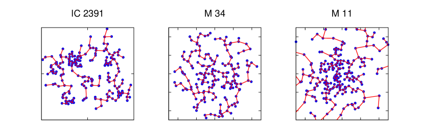
Figure 2: Minimum spanning trees for three open clusters, from which the parameter $Q$ can be calculated (see text). Star positions are indicated with blue circles and red lines represent the trees. The value of $Q$ quantifies the spatial distribution of stars. For IC 2391 the stars are distributed following an irregular, fractal pattern ($Q=0.66<0.8$), for M 34 the stars are distributed roughly homogeneously ($Q=0.8$), and for M 11 the stars follow a radial density profile ($Q=1.02>0.8$).

It is expected that the internal structure of a star cluster evolves with time from initial fractal clustering ($Q<0.8$) to either homogeneous distribution ($Q\simeq 0.8$) if the cluster is dispersing its stars or centrally concentrated distribution ($Q>0.8$) if it is a bound cluster. Cartwright & Whitworth (2004) calculated $Q$ FOR several star clusters. They obtained $Q=0.47$ for stars in Taurus, a value consistent with its observed clumpy structure and with its relatively young evolutionary stage (they estimated an age in crossing time units of $T/T_{cross}\simeq 0.1$). However, they also found some apparent contradictory results. IC 348, a slightly evolved cluster with $T/T_{cross}\simeq 1$ yielded $Q=0.98$ according to its steep radial density profile. Instead, the highly evolved cluster IC 2391 ($T/T_{cross}\simeq 20$) still exhibits fractal clustering with $Q=0.66$. Schmeja et al. (2008) applied this technique to embedded clusters in the Perseus, Serpens and Ophiuchus molecular clouds, and found that older Class 2/3 objects are more centrally condensed than the younger Class 0/1 protostars. Sánchez & Alfaro (2009) measured $Q$ in a sample of $16$ open clusters in the Milky Way spanning a wide range of ages. They found that there can exist clusters as old as $\sim 100$ Myr exhibiting fractal structure. This means that either the initial clumpiness may last for a long time or other mechanisms may develop some kind of substructure starting from an initially more homogeneous state. Sánchez & Alfaro (2009) obtained a statistically significant correlation between $Q$ and $T/T_{cross}$ in their sample of open clusters. Figure 3a shows

Figure 3: (a) Structure parameter as a function of the logarithm of age in crossing time units. Dashed line separates radial from fractal clustering and solid line is the best linear fit. (b) Correlation dimension as a function of age in crossing-time units. The best linear fit is represented by a solid line. For reference, a horizontal dashed line indicates the value corresponding to three-dimensional distributions with fractal dimensions of $D_{f}=2.0$.

this tendency where the crossing times were calculated by assuming a constant velocity dispersion of $2$ km s^-1. As we can see, the general trend is that young clusters (meaning that dynamically less evolved clusters) tend to distribute their stars following fractal patterns whereas older clusters tend to exhibit centrally concentrated structures. This result support the idea that stars in newly born clusters likely follow the fractal patterns of their parent molecular clouds, and that they eventually evolve towards more centrally concentrated structures. However, we know that this is only an overall trend. Some very young clusters may exhibit radial density gradients, as for instance $\sigma$ Orionis for which $Q\simeq 0.9$ (Caballero 2008).

Given the wide variety of physical processes involved in the origin and early evolution of star clusters, it is somewhat surprising that a correlation like that seen in Figure 3a can be observed. Very recent simulations by Allison et al. (2009, 2010) and Moeckel & Bate (2010) show that the transition from fractal clustering to central clustering may occur on very short timescales ($\lesssim 1$ Myr). Simulations by Maschberger et al. (2010) suggest a more complex variety of possibilities. Bound systems may start fractal and evolve towards a centrally concentrated stage whereas unbound systems may stay fractal in time. But this is the evolution for the whole systems. Star clusters in each system may evolve in totally different ways. In fact, the time evolution of the $Q$ parameter of clusters fluctuates dramatically depending on episodes of relaxation or merging (see Figure $8$ in Maschberger et al. 2010). It is difficult to argue that, despite all this complex formation history (occurring in $\sim 0.5$ Myr), we should still observe some correlation between internal structure and age.

6 Initial fractal dimension of star clusters

For those open clusters with internal substructure, the fractal dimension also shows a significant correlation with the age in crossing time units (Sánchez & Alfaro 2009), as it can be seen in Figure 3b. The degree of clumpiness is smaller for more evolved clusters. The horizontal dashed line in Figure 3b shows a reference $D_{f}$ value estimated from previous papers (Sánchez & Alfaro 2008). It is interesting to note that open clusters with the smallest correlation dimensions $D_{c}=1.74$ would have 3D fractal dimensions around $D_{f}\sim 2$. This value is considerably smaller than the average value estimated for Galactic molecular clouds (see Section $2$), which is $D_{f}\simeq 2.6-2.8$.

This result creates an apparent problem to be addressed, because as mentioned before a group of stars born from the same cloud at almost the same place and time is expected to have a fractal dimension similar to that of the parent cloud. If the fractal dimension of the interstellar medium has a nearly universal value around $2.6-2.8$, then how can some clusters exhibit such small fractal dimensions? This is still an open question. Several possibilities should be investigated in future studies. First, some simulations demonstrate that it is possible to increase the clumpiness (to decrease $D_{f}$) with time (Goodwin & Whitworth 2004). Second, maybe this difference is a consequence of a more clustered distribution of the densest gas from which stars form on the smallest spatial scales in the molecular cloud complexes, according to a multifractal scenario (Chappell & Scalo 2001). Third, perhaps the star formation process itself modifies in some (unknown) way the underlying geometry generating distributions of stars that can be very different from the distribution of gas in the star-forming cloud. A fourth possibility is that the fractal dimension of the interstellar medium in the Galaxy does not have a universal value (i.e., that $D_{f}$ is different from region to region depending on the main physical processes driving the turbulence). Therefore some clusters could show smaller initial fractal dimensions because they formed in more clustered regions. The possibility of a non-universal fractal dimension for the ISM should not, in principle, be ruled out. However, in this last case, overall correlations as those shown in Figures 3a and 3b should not, in principle, be observed.

References

- [1] Allison, R.J., Goodwin, S.P., Parker, R.J. et al. 2009, ApJ (Letters), 700, L99
- [2] Allison, R.J., Goodwin, S.P., Parker, R.J. et al. 2010, MNRAS, in press (arXiv:1004.5244).
- [3] Bate, M.R., Clarke, C.J., McCaughrean, M.J. 1998, MNRAS, 297, 1163
- [4] Bazell, D., Desert, F.X. 1988, ApJ, 333, 353
- [5] Beech, M. 1987, Ap&SS, 133, 193
- [6] Beech, M. 1992, Ap&SS, 192, 103
- [7] Bergin, E.A., Tafalla, M. 2007, ARAA, 45, 339
- [8] Bonnell, I. A., Bate, M. R., Vine, S. G. 2003, MNRAS, 343, 413
- [9] Caballero, J.A. 2008, MNRAS 383, 375
- [10] Cartwright, A., Whitworth, A.P. 2004, MNRAS, 348, 589
- [11] Chappell, D., Scalo, J. 2001, ApJ, 551, 712
- [12] de la Fuente Marcos, R., de la Fuente Marcos, C. 2006, A&A, 452, 163
- [13] de la Fuente Marcos, R., de la Fuente Marcos, C. 2009, ApJ, 700, 436
- [14] Dickman, R.L., Horvath, M.A., Margulis, M. 1990, ApJ, 365, 586
- [15] Efremov, Y.N. 1995, AJ, 110, 2757
- [16] Elias, F., Alfaro, E.J., Cabrera-Caño, J. 2009, MNRAS, 397, 2
- [17] Elmegreen, B.G., 2010, IAU Symposium, 266, 3
- [18] Elmegreen, B.G., Scalo, J. 2004, ARAA, 42, 211
- [19] Falgarone, E., Phillips, T.G., Walker, C.K. 1991, ApJ, 378, 186
- [20] Gieles, M. 2010, IAU Symposium, 266, 6
- [21] Gladwin, P.P., Kitsionas, S., Boffin, H.M.J. et al. 1999, MNRAS, 302, 305
- [22] Goodwin, S.P., Whitworth, A.P. 2004, A&A, 413, 929
- [23] Hartmann, L. 2002, ApJ, 578, 914
- [24] Hetem, A.Jr., Lepine, J.R.D. 1993, A&A, 270, 451
- [25] Kraus, A.L., Hillenbrand, L.A. 2008, ApJ (Letters), 686, L111
- [26] Lada, C.J., Lada, E.A. 2003, ARAA, 41, 57
- [27] Larson, R.B. 1981, MNRAS, 194, 809
- [28] Larson, R.B. 1995, MNRAS, 272, 213
- [29] Larson, R.B. 2007, Reports on Progress in Physics, 70, 337
- [30] Lee, Y. 2004, Journal of Korean Astronomical Society, 37, 137
- [31] Lee, Y., Kang, M., Kim, B.K. et al. 2008, Journal of Korean Astronomical Society, 41, 157
- [32] Maíz-Apellániz, J. 2001, ApJ, 563, 151
- [33] Mandelbrot, B.B. 1983, in: The Fractal Geometry of Nature (New York: Freeman)
- [34] Maschberger, T., Clarke, C.J., Bonnell, I.A. et al. 2010, MNRAS, 404, 1061
- [35] Moeckel, N., Bate, M.R. 2010, MNRAS, 404, 721
- [36] Nakajima, Y., Tachihara, K., Hanawa, T. et al. 1998, ApJ, 497, 721
- [37] Sánchez, N., Alfaro, E.J., Pérez, E. 2005, ApJ, 625, 849
- [38] Sánchez, N., Alfaro, E.J., Pérez, E. 2007a, ApJ, 656, 222
- [39] Sánchez, N., Alfaro, E.J., Elias, F. et al. 2007b, ApJ, 667, 213
- [40] Sánchez, N., Alfaro, E.J. 2008, ApJS, 178, 1
- [41] Sánchez, N., Alfaro, E.J. 2009, ApJ, 696, 2086
- [42] Schmeja, S., Klessen, R.S. 2006, A&A, 449, 151
- [43] Schmeja, S., Kumar, M.S.N., Ferreira, B. 2008, MNRAS, 389, 1209
- [44] Simon, M. 1997, ApJ (Letters), 482, L81
- [45] Stutzki, R. 1993, Reviews in Modern Astronomy, 6, 209
- [46] Vogelaar, M.G.R., Wakker, B.P. 1994, A&A, 291, 557