Lattice effects in the scaling limit
of the two-dimensional self-avoiding walk

Abstract

We consider the two-dimensional self-avoiding walk (SAW) in a simply connected domain that contains the origin. The SAW starts at the origin and ends somewhere on the boundary. The distribution of the endpoint along the boundary is expected to differ from the SLE partition function prediction for this distribution because of lattice effects that persist in the scaling limit. We give a precise conjecture for how to compute this lattice effect correction and support our conjecture with simulations. We also give a precise conjecture for the lattice corrections that persist in the scaling limit of the $\lambda$-SAW walk.

1 Introduction

Let $D$ be a bounded, simply connected domain in the complex plane that contains $0$. We are interested in the self-avoiding walk (SAW) in $D$ starting at the origin and ending on the boundary of $D$. It is defined as follows. We introduce a lattice with spacing $\delta>0$, e.g., $\delta{\mathbb{Z}}^{2}$. A self-avoiding walk is a nearest neighbor walk on the lattice with the property that it does not visit any site more than once. To be precise, let ${\mathcal{W}}(D,\delta)$ denote the set of functions of the form $\omega:\{0,1,2,\cdots,n\}\rightarrow\delta{\mathbb{Z}}^{2}$ where $n$ is a positive integer; $||\omega(i)-\omega(i-1)||=\delta$ for $i=1,2,\cdots,n$; $\omega(i)\neq\omega(j)$ for $0\leq i<j\leq n$; $\omega(0)=0$; $\omega(j)\in D,j<n$; $\omega(n)\not\in D$. The integer $n$ is the number of steps in the SAW, and from now on we will denote it by $|\omega|$.

Since ${\mathcal{W}}(D,\delta)$ is finite, we can define a probability measure on ${\mathcal{W}}(D,\delta)$ by taking the probability of $\omega$ to be proportional to $\beta^{|\omega|}$ where $\beta>0$ is a parameter. So

$${\bf P}(\omega)={\bf P}_{D,\delta}(\omega)={\beta^{|\omega|}\over Z(D)}$$ (1)

where the partition function $Z(D)=Z_{\delta}(D)$ is defined by the requirement that this be a probability measure. One can consider this model for all $\beta>0$, but it is most interesting for one particular value that makes the model critical, $\beta=1/\mu$, where $\mu$ is the connective constant which we define next.

Let $c_{N}$ be the number of SAW’s in the lattice with $N$ steps that start at $0$. (They are not constrained to lie in $D$.) It is known that this number grows exponentially with $N$ in the sense that the following limit exists [13].

$$\mu=\lim_{N\rightarrow\infty}c_{N}^{1/N}.$$ (2)

The connective constant $\mu$ depends on the lattice. Nienhuis [14] predicted that for the hexagonal lattice $\mu=\sqrt{2+\sqrt{2}}$, and this was recently proven by Duminil-Copin and Smirnov [4]. For the square and triangular lattices there are only numerical estimates of the value of $\mu$. For the remainder of this paper we will take $\beta=1/\mu$ to make the model critical.

We also consider the analogy of the above definition with the ordinary random walk. The natural way to describe the random walk in $D$ starting at $0$ and ending on the boundary of $D$ is to start a random walk at $0$ and run it until it hits the boundary. Let ${\mathcal{S}}(D,\delta)$ be the set of such walks. The probability of a particular such random walk $\omega$ is ${z}^{-|\omega|}$ where ${z}$ is the coordination number of the lattice, e.g., ${z}=4$ for the square lattice. We can consider this as a random walk starting at the origin stopped when it leaves $D$, or just as a measure on ${\mathcal{S}}(D,\delta)$ that assigns measure $z^{-n}$ to each walk of length $n$. In the SAW the connectivity constant $\mu$ plays the role of the coordination number $z$ for the random walk.

In both the SAW and the ordinary random walk we are interested in the scaling limit in which the lattice spacing $\delta\rightarrow 0$. Let us first discuss the case of ordinary random walk which is well understood.

For the ordinary random walk the scaling limit is Brownian motion starting at $0$ and stopped when it hits the boundary of $D$. The distribution of the endpoint of the Brownian motion on the boundary is harmonic measure. The lattice effects associated to the definition of the first boundary point of the lattice walk disappear in the scaling limit. The key fact is that if a random walk or a Brownian motion gets very close to the boundary, then it will hit it soon. Therefore, if we couple a random walk and a Brownian motion on the same probability space so the paths are close, then the first time that the random walk hits the boundary will be close to the first time that the Brownian motion hits the boundary. See [8, Section 7.7] for a precise statement. The argument there works for any simply connected domain even with nonsmooth boundaries, and extends to finitely connected domains as well. One does need to assume that the boundary is sufficiently large so that when the Brownian motion or random walk gets close, then it is very likely to hit it soon.

If the boundary of our domain $D$ is a piecewise smooth curve, then harmonic measure is absolutely continuous with respect to arc length along the boundary [15]. We let $h_{D}(z)$ denote its density with respect to arc length; this is often called the Poisson kernel (starting at $0$). If $f$ is a conformal map on $D$ that fixes the origin and such that the boundary of $f(D)$ is also piecewise smooth, then the conformal invariance of Brownian motion [12] implies that the density for harmonic measure on the boundary of $f(D)$ is related to the density on the boundary of $D$ by

$$h_{D}(z)=|f^{\prime}(z)|h_{f(D)}(f(z)).$$ (3)

If $D$ is simply connected and we take $g_{D}$ to be a conformal map of $D$ onto the unit disc which fixes $0$, then by symmetry $h_{f(D)}(f(z))$ is just $1/2\pi$, and so $h_{D}(z)=|g_{D}^{\prime}(z)|/2\pi$. We emphasize that conformal invariance of harmonic measure implies that the exponent of $|f^{\prime}(z)|$ in (3) equals one.

We now consider the SAW in $D$ from the origin to the boundary of $D$. Here we will assume that $\partial D$ is piecewise smooth. In this case we have the following conjecture.

• As $\delta\rightarrow 0$, the measures ${\bf P}_{D,\delta}$ converge to a probability measure ${\bf P}_{D}$ on simple paths from the origin to $\partial D$.

• The measure ${\bf P}_{D}$ can be written as

  $$\int_{\partial D}\tilde{\rho}_{D}(z)\,{\bf P}_{D}(0,z)\,|dz|,$$ (4)

  where $\tilde{\rho}_{D}(z)$ is the density of a probability measure on $\partial D$ and ${\bf P}_{D}(0,z)$ is the probability measure associated to radial $SLE_{8/3}$ from $0$ to $z$ in $D$.

• There exists a periodic function, $l(\theta)$, such that

  $$\tilde{\rho}_{D}(z)=l(\theta(z,D))\,\rho_{D}(z)$$ (5)

  where $\theta(z,D)$ is the angle of the tangent to $\partial D$ at $z$ and $\rho_{D}(z)$ is a multiple of the $SLE_{8/3}$ partition function. The function $l(\theta)$ and its period depend on the lattice. For example, on the square lattice the period is $\pi/2$.

• The density $\rho_{D}(z)$ transforms under conformal maps by

  $$\rho_{D}(z)=c|f^{\prime}(z)|^{5/8}\rho_{f(D)}(f(z))$$ (6)

  The constant $c$ is determined by the constraint that this be a probability density. (It depends on $D$ and $f$.) In particular, if $D$ is simply connected, and $g_{D}:D\rightarrow\mathbb{D}$ with $g_{D}(0)=0$, then

  $$\rho_{D}(z)=c|g_{D}^{\prime}(z)|^{5/8}$$ (7)

  ($\mathbb{D}$ denotes the unit disc centered at the origin.)

In the case of ${\mathbb{Z}}^{2}$ where the boundary of $D$ is composed of horizontal and vertical line segments, this conjecture was made by Lawler, Schramm and Werner [10]. Simulations on an infinite horizontal strip [3] give strong support to the conjecture. For such boundaries, $l(\theta(z,\theta))$ is constant. The conjecture was reiterated in [9] where it was also conjectured for other domains “…after taking care of the local lattice effects.” Our conjecture makes precise the nature of the lattice effects in terms of the lattice correction $l(\theta(z,\theta))$. The function $l(\theta)$ will depend on just how we define “ending on the boundary of $D$” and on the lattice type. In general, we use $\rho$ to denote densities that do not include the lattice effects that persist in the scaling limit, e.g., (6), and we use $\tilde{\rho}$ to denote densities that do include the lattice effects, e.g., (5).

Unfortunately, the Monte Carlo algorithms for simulating the above ensemble are local algorithms and so are not very efficient [13]. We have not attempted to test the conjecture for this ensemble by simulation. Instead we introduce another ensemble that we can study with the pivot algorithm, a fast global Monte Carlo algorithm. Instead of stopping a walk at a boundary point, one chooses an infinite length walk conditioned on the event that it crosses the boundary only once. We will refer to this ensemble as the “cut-curve” ensemble since the boundary of the domain cuts the SAW into two SAW’s, one contained in $D$ and one in the complement of $D$. The above ensemble and the cut-curve ensemble are the same for the infinite strip studied in [3], but for most domains this is not the case.

The scaling limits of the SAW and the loop-erased walk, which is obtained by erasing loops from the ordinary random walk, are two cases of the Schramm-Loewner evolution (SLE). The discrete models can be considered as special cases of the $\lambda$-SAW. We review the $\lambda$-SAW in the next section, and we extend our conjecture to this case. (There is no precise conjecture in the literature on the nature of the lattice correction, and we think it is worthwhile to write it down.) After that we consider the conjectured scaling limits of the two ensembles — walks stopped upon reaching the boundary and walks conditioned to hit the boundary only once. In only the $\kappa=8/3$ (SAW) case do we expect an equivalence of these ensembles, and therefore the tests we do here would not work for other values of $\kappa$.

In section two we return to the SAW and give explicit conjectures for the lattice correction function $l(\theta)$ for the two lattice ensembles. In section three, we discuss simulations for the cut-curve ensemble including numerical calculation of the lattice correction function. In the final section we summarize our results and discuss the lattice correction function $l(\theta)$ for other interpretations of the SAW ending on the boundary of the domain.

1.1 $\lambda$-SAW

The conjectures for the SAW and the results for the ordinary walk (considered in terms of the loop-erasure of the paths) are particular cases of conjectures for a model called the $\lambda$-SAW introduced by Kozdron and Lawler [6]. Even though we are only testing the SAW conjecture, we will give the conjectures for the general model. There are two versions, chordal (boundary-to-boundary) and radial (boundary-to-interior); we will restrict our discussion here to the radial case. (There is also an interior-to-interior case, but then there is no boundary lattice correction so it is not relevant for this paper.) As above, we assume that $D$ is a domain with piecewise smooth boundary. For convenience we use ${\mathbb{Z}}^{2}$ for our lattice, but the definition can be extended to other lattices. The parameter $\lambda$ can be considered a free parameter, but we will set $\lambda=-{\bf c}/2$ where ${\bf c}\leq 1$ denotes central charge. (We will not define central charge in this paper and can just take it as a parameter.) The $\lambda$-SAW is a model that is conjectured to have a scaling limit of $SLE_{\kappa}$ where

$$\kappa=\frac{13-{\bf c}-\sqrt{(13-{\bf c})^{2}-144}}{3}\in(0,4].$$

The (rooted) random walk loop measure is the measure on ordinary random walk loops that assigns weight $(1/4)^{n}\,n^{-1}$ to each loop of $n>0$ steps. A loop is a path which begins and ends at the same point. The measure can also be considered as a measure on unrooted loops by forgetting the root.

For each lattice spacing $\delta$ and each SAW $\omega$ as above, we let $m_{D}(\omega)$ denote the total measure of the set of loops that lie entirely in $D$ and share at least one site with $\omega$. If $\beta>0$, the $\lambda$-SAW gives each SAW $\omega$ as above weight

$$q(\omega)=q_{\delta,D,{\bf c},\beta}(\omega)=\beta^{|\omega|}\,\exp\left\{-\frac{{\bf c}}{2}\,m_{D}(\omega)\right\}.$$

The partition function is

$$Z(D;\delta)=Z(D;\delta,{\bf c},\beta)=\sum{q(\omega)},$$

where the sum is over all SAWs on the lattice $\delta{\mathbb{Z}}^{2}$ that start at the origin and end at the boundary. (As noted before, there are several definitions for “ending at the boundary”. In the discussion here, we fix one such definition and the lattice-dependent quantities depend on the choice.) It is conjectured that for each ${\bf c}$, there is a critical value $\beta=\beta_{\bf c}$ such that $Z(D;\delta)$ follows a power law in $\delta$ as $\delta\rightarrow 0$. We assume this conjecture and fix $\beta$ at the critical value.

If ${\bf c}=0$, then this is the usual SAW model. If ${\bf c}=-2$, then this is the loop-erased random walk (LERW) which is obtained by taking the ordinary random walk as above and erasing loops chronologically from the paths. The partition function $Z(D;\delta)$ for the loop-erased walk is exactly the same as that for the usual random walk. (See [8, Chapter 9] for a discussion of this.) We state our conjectures in terms of the boundary and interior scaling exponent for $SLE_{\kappa}$:

$$b=\frac{6-\kappa}{2\kappa}\in[1/4,\infty),\;\;\;\;\tilde{b}=\frac{b\,(\kappa-2)}{4}.$$

• There is a lattice correction function $l(\theta)$ that is continuous, strictly positive and periodic.

• If $\omega$ is from $0$ to $\partial D$, let $l(\omega)$ denote $l(\theta(z,D))$ where $z$ is the first point on $\partial D$ hit by a bond of $\omega$ and $\theta(z,D)$ is the angle of the tangent to $\partial D$ at $z$. Define the lattice-corrected weight by

  $$\hat{q}(\omega)=\frac{q(\omega)}{l(\omega)}.$$

• As $\delta\rightarrow 0$, the measure $\delta^{1-b-\tilde{b}}\,\hat{q}$ on paths converges to a nontrivial finite measure $\nu_{D}$ on simple paths from $0$ to $\partial D$. It can be written as

  $$\nu_{D}=\int_{\partial D}\rho_{D}(z)\,\nu_{D}^{\#}(0,z)\,|dz|,$$

  where $\rho_{D}$ is a positive function and $\nu_{D}^{\#}(0,z)$ is a probability measure on simple paths starting at $0$ and leaving $D$ at $z$.

• If $g$ is a conformal transformation with $g(0)=0$ that is smooth on $\partial D$, then

  $$\rho_{D}(z)=|g^{\prime}(z)|^{b}\,|g^{\prime}(0)|^{\tilde{b}}\,\rho_{g(D)}(z).$$ (8)

• The probability measures $\nu_{D}^{\#}(0,z)$, considered as measures on curves modulo reparametrization, are conformally invariant. More specifically, if $\gamma:[0,t_{0})\rightarrow D$ is a curve with $\gamma(t_{0}-)\in\partial D$, let

  $$\sigma(t)=\int_{0}^{t}|g^{\prime}(\gamma(s))|^{d}\,ds,\;\;\;\;d=1+\frac{\kappa}{8},$$

  and define $g\circ\gamma(t)$ by

  $$g\circ\gamma(\sigma(t))=g(\gamma(t)),\;\;\;\;0\leq t\leq\sigma(t_{0}).$$

  If $g\circ\mu^{\#}_{D}(0,z)$ denotes the induced measure on curves on $g(D)$, then

  $$g\circ\nu_{D}^{\#}(0,z)=\nu_{g(D)}^{\#}(0,z).$$

• If $D$ is simply connected, then $\nu_{D}^{\#}(0,z)$ is the reversal of radial $SLE_{\kappa}$ from $z$ to $0$ in $D$ with the natural parametrization. (This should also be true for multiply connected $D$ under the appropriate definition of $SLE_{\kappa}$ proposed in [7].)

These conjectures are a long way from being proved. Indeed, a special case is the SAW model which is a notoriously difficult problem! However, we state them here to see that the precise conjecture requires discussing a boundary lattice correction; our conjecture is that the correction only depends on the angle of the boundary. We make a number of comments.

• The density $\rho_{D}(z)$ is sometimes called the partition function for radial $SLE_{\kappa}$. It is defined up to an arbitrary constant.

• The loop-erased walk (${\bf c}=-2$) is particularly nice because it is closely related to the ordinary random walk. The partition function is the Poisson kernel (density of harmonic measure) even for non-simply connected domains.

• For other values of ${\bf c}$, if $D$ is simply connected, the partition function is the Poisson kernel raised to the $b$th power. However, this is not true for multiply connected domains.

• The loop terms $m_{D}(\omega)$ can be considered as having three parts. The very small loops that occur away from the boundary contribute a microscopic (lattice dependent) part that affects the critical value of $\beta$. The large loops contribute a macroscopic term that is seen in the scaling limit; this is the Brownian loop measure as defined in [11]. Finally, there are the small loops that occur near the boundary. They give both a macroscopic effect seen in the exponent $b$ and a microscopic effect in the function $l$. The boundary effect is measured both in the number of walks that stay one one side of a line and in the measure of loops that go on the walks. We only see the first effect in the SAW (${\bf c}=0$) case.

• If $\kappa=8/3$, then $b=5/8,\tilde{b}=5/48$. There is a $|g^{\prime}(0)|^{\tilde{b}}$ factor in (8) that does not seem to appear in (6). However, it is implicitly there in the normalization to make the measure a probability measure.

1.2 Cut-curve configurations

We will be testing a cut-curve ensemble for SAW’s. The case ${\bf c}=0$, which is what we use in this paper, is special for such configurations and agrees with the bridge decomposition of restriction measures [1], but for the sake of completeness let us discuss the general case for ${\bf c}\leq 1$. Suppose $D$ is a bounded, simply connected domain containing the origin whose boundary $\partial D$ is a smooth Jordan curve. Let $D^{*}$ be the unbounded component of ${\mathbb{C}}\setminus\partial D$. We consider two measures on simple curves from $0$ to infinity that intersect $\partial D$ only once:

1. Take “whole-plane” $SLE_{\kappa}$ and condition on the event that the curve intersects $\partial D$ only once. This is conditioning on an event of probability zero, so one must define this in terms of a limit.

2. Take independent copies of radial $SLE_{\kappa}$ in $D$ and in $D^{*}$ and condition them to hit the same point in $\partial D$. Then concatenate the paths.

In order to see the difference, let us describe the lattice models that we expect to converge to these measures. Since it is hard to talk about infinite walks, we will choose a point $z^{*}\in D^{*}$ with large absolute value. We take the scaling limit for fixed $z^{*}$ and then let $z^{*}$ go to infinity. If $\delta$ is a scaling factor, we abuse notation slightly and write $z^{*}$ for the point in $\delta{\mathbb{Z}}^{2}$ closest to $z^{*}$. We consider two measures on paths. For each $\delta$, we consider the set ${\mathcal{W}}(\delta,D,z^{*})$ of SAW’s $\omega$ on $\delta{\mathbb{Z}}^{2}$ with $\omega(0)=0,\omega(|\omega|)=z^{*}$, $|\omega(j)|\leq|z^{*}|^{2}$ for all $j$ such that there exists only one bond that intersect $\partial D$. We write $z_{\omega},w_{\omega}$ for the vertices in this bond with $z_{\omega}\in D,w_{\omega}\in{\mathbb{C}}\setminus D$, and we write $\omega=\omega^{D}\oplus[z_{\omega},w_{\omega}]\oplus\omega^{*}$ where

$$\omega^{D}=[\omega(0),\ldots,z_{\omega}],\;\;\;\;\omega^{*}=[w_{\omega},\ldots,\omega(|\omega|)].$$

Let $\beta=\beta_{\bf c}$ be the critical value. Then we consider the following measures on ${\mathcal{W}}(\delta,D,z^{*})$:

1. Each $\omega$ gets weight

   $$q_{1}(\omega)=\beta^{|\omega|}\,\exp\left\{-\frac{{\bf c}}{2}m(\omega;z^{*})\right\},$$

   where $m(\omega;z^{*})$ denotes the measure of loops staying in the ball of radius $|z^{*}|^{2}$ that intersect $\omega$.

2. Each $\omega$ gets weight

   $$q_{2}(\omega)=\beta^{|\omega|}\,\exp\left\{-\frac{{\bf c}}{2}[m_{D}(\omega^{D})+m_{D^{*}}(\omega^{*})]\right\}$$

We can state our conjectures as follows. Let $\theta(\omega)$ be the angle of the tangent to $\partial D$ at the point where $\omega$ hits $\partial D$.

1. There exists a lattice correction function $\hat{l}_{1}$ such that we can take the scaling limit of the measure

   $$\hat{q}_{1}(\omega)=\frac{q_{1}(\omega)}{\hat{l}_{1}(\omega)}.$$

   If we then take $z^{*}\rightarrow\infty$, we get whole plane $SLE_{\kappa}$ conditioned to hit $\partial D$ only once.

2. There exists a lattice correction function $\hat{l}_{2}$ such that the scaling limit of the measure

   $$\hat{q}_{2}(\omega)=\frac{q_{2}(\omega)}{\hat{l}_{2}(\omega)}$$

   exists. If we then take $z^{*}$ to infinity, we get the measure given by

   $$c\int_{\partial D}\rho_{D}(z)\,\rho_{D}^{*}(z)\,\left[\nu_{D}^{\#}(0,z)\oplus\nu_{D^{*}}^{\#}(z,\infty)\right]\,|dz|.$$

   Here $\rho^{*}(z)$ is the density as in (8) for radial $SLE_{\kappa}$ in $D^{*}$ centered at infinity.

For ${\bf c}=0$ (restriction measures), the two limits agree and this is what we use for SAW in this paper. For other values of ${\bf c}$ we get different measures. For example if ${\bf c}=-2$ (loop-erased walk), the first measure corresponds to loop-erased walk conditioned to hit $\partial D$ only once and the second measure corresponds to the loop-erasure of an ordinary walk conditioned to hit $\partial D$ only once.

2 Lattice effects

The constraint that the SAW stays in $D$ has both a macroscopic and a microscopic effect on the boundary density. The macroscopic effect is captured by the conjecture (6). The microscopic effect comes from the behavior near the endpoint of the walk on the boundary of $D$. Consider a SAW that ends at $z\in\partial D$ and consider the tangent line to the boundary at $z$. The constraint that the SAW stays in $D$ implies that near $z$ the SAW must stay on one side of this line. Loosely speaking, the number of SAW’s that end at $z$ and stay on one side of this line depends on the orientation of the line with respect to the lattice. The result is a factor $l(\theta)$ that depends on the angle of the tangent line with respect to the lattice, and so we obtain our conjecture (5).

The lattice correction function $l(\theta)$ depends on the type of lattice and on how we interpret “ending on the boundary of $D$.” We will first discuss the interpretation we introduced at the start of the introduction. We consider all SAW’s $\omega$ with $\omega(0)=0$, $\omega(i)\in D$ for $i=0,1,2,\cdots,|\omega|-1$ and $\omega(|\omega|)\notin D$. ($|\omega|$ denotes the number of steps in $\omega$.) So the last bond of the SAW intersects the boundary of $D$, and this is the only bond in the SAW that intersects the boundary.

We can compute the lattice correction function $l(\theta)$ as follows. We give the details for the square lattice. Other lattices, e.g., the triangular or hexagonal, will require some modifications. Consider a bond that intersects the boundary $\partial D$. Let $z$ be the endpoint of the bond that is in $D$. Let $w$ be the point where the bond intersects the boundary (typically not a lattice site). Consider the tangent line to the boundary at $w$. We need to count the number of SAW’s of a fixed length $N$ that end at $z$ and do not intersect this tangent line. This quantity will depend on the angle of the tangent line with respect to the lattice. It will also depend on the distance $|w-z|$ and on whether the bond is horizontal or vertical. However, these two factors are the only dependence on the bond.

Motivated by the above, we consider the vertical bond between $(0,0)$ and $(0,1)$. We fix an $l$ in the interval $[0,1]$ and an angle $\theta$. The parameter $l$ plays the role of the distance $|w-z|$. Let $L$ be the line with polar angle $\theta$ passing through the point $(0,l)$. We consider SAW’s with $N$ steps ending at the origin which by reversal can be considered as beginning at the origin. Let $c_{N}$ be the number of such walks, and let $a_{N}(l,\theta)$ be the number of such walks that do not intersect the line. So $a_{N}(l,\theta)/c_{N}$ is the probability that the $N$ step SAW does not intersect the line. We expect that there exists a function $p^{v}(l,\theta)$ such that

$${a_{N}(l,\theta)\over c_{N}}\sim p^{v}(l,\theta)\,N^{-\rho},\quad N\rightarrow\infty$$

with $\rho=25/64$ [10]. The actual exponent is not important here. The key is that if $l^{\prime},\theta^{\prime}$ are two different values, then

$$\frac{a_{N}(l,\theta)}{a_{N}(l^{\prime},\theta^{\prime})}\sim\frac{p^{v}(l,\theta)}{p^{v}(l^{\prime},\theta^{\prime})},\quad N\rightarrow\infty.$$

We define

$$p^{v}_{1}(l,\theta)=\lim_{N\rightarrow\infty}{a_{N}(l,\theta)\over c_{N}}N^{\rho}$$ (9)

(We do not know how to prove this limit exists.) The superscript $v$ on $p$ indicates that we took the bond crossing the boundary to be vertical. We use the subscript $1$ to distinguish the quantities related to the lattice correction function for this particular ensemble from the ensemble that we will consider next. We let $p^{h}_{1}$ denote the analogous quantity for a horizontal bond. The symmetry of the square lattice implies that $p_{1}^{h}(l,\theta)=p^{v}_{1}(l,\theta+\pi/2)$. (Note that $p^{h}_{1}(l,\theta)$ and $p^{v}_{1}(l,\theta)$ have period $\pi$ in $\theta$.)

Now consider what happens as we move along the boundary. The angle $\theta$ of the tangent will vary smoothly. The distance $l$ will not. As long as $\tan(\theta)$ is not rational, $l$ will be distributed uniformly between $0$ and $1$. So in the scaling limit, averaging over an infinitesimal section of the boundary will be equivalent to averaging $l$ over $[0,1]$. So we define

$$p_{1}^{x}(\theta)=\int_{0}^{1}p_{1}^{x}(l,\theta)\,dl,\quad x=h,v$$

The function $p^{x}_{1}(\theta)$ captures the microscopic lattice effect caused by the constraint that the SAW must stay on one side of a line as it approaches the boundary. There is another lattice effect that comes from the density of bonds that cross the boundary. Define $b^{v}(\theta)$ to be the density of vertical bonds along a line with polar angle $\theta$, i.e., the average number of vertical bonds that intersect the line per unit length. We have $b^{v}(\theta)=|\cos(\theta)|$. The density of horizontal bonds $b^{h}(\theta)$ is $b^{v}(\theta-\pi/2)=|\sin(\theta)|$. The lattice correction function is then

$$l_{1}(\theta)=b^{v}(\theta)p^{v}_{1}(\theta)+b^{h}(\theta)p^{h}_{1}(\theta)$$ (10)

and the boundary density for this first interpretation of ending on the boundary is

$$\tilde{\rho}_{D,1}(z)=\tilde{c_{1}}|g_{D}^{\prime}(z)|^{5/8}l_{1}(\theta(z,D))$$ (11)

The Monte Carlo algorithms for simulating the above ensemble are local algorithms and so are not very efficient [13]. We have not attempted to test the conjecture for this ensemble by simulation. Instead we use the cut-curve ensemble introduced earlier. We consider the infinite length SAW in the full plane starting at $0$. We condition on the event that the SAW crosses the boundary of $D$ exactly once. Consider a bond crossing the boundary, and let $z$ be the endpoint inside $D$ and $w$ the endpoint outside of $D$. If we condition on the event that the SAW contains this particular bond and this is the only bond in the SAW that crosses the boundary, then we have a SAW in $D$ from $0$ to $z$ and a SAW in the exterior of $D$ from $w$ to $\infty$. So the conjecture for the boundary density will be a product of two functions. The interior SAW from $0$ to $z$ gives a factor of $\rho_{D}(z)$ with $\rho_{D}(z)$ given by (6). The exterior SAW from $w$ to $\infty$ gives a factor of $\rho^{*}_{D}(z)$ given by

$$\rho^{*}_{D}(z)=c|h^{\prime}_{D}(z)|^{5/8}$$

where $h_{D}(z)$ is the conformal map of $D^{*}$ onto the unit disc $\mathbb{D}$ with $h_{D}(\infty)=0$. Our conjecture for the density of the point where the SAW crosses the curve is

$$\tilde{\rho}_{D,2}(z)=\rho_{D}(z)\,\rho^{*}_{D}(z)\,l_{2}(\theta(z,D)),$$ (12)

where $l_{2}(\theta)$ is the lattice correction function for the cut-curve ensemble. (The subscript $2$ indicates that the quantities are for the cut-curve ensemble.)

We can compute $l_{2}(\theta)$ as follows. Again, we restrict our attention to the square lattice. For $l\in[0,1]$ and an angle $\theta$, let $L$ be the line with polar angle $\theta$ passing through $(0,l)$. We consider SAW’s with $N=2n+1$ steps such that the middle bond is the bond between $(0,0)$ and $(0,1)$. Let $d_{N}$ be the number of such walks, and let $b_{N}(l,\theta)$ be the number of such walks that only intersect the line once. (Of course it must be the middle bond that has the intersection). (By translating our SAW’s so that they start at $0$, we see that $d_{N}=c_{N}/2$.) Note that $b_{N}(l,\theta)/d_{N}$ is the probability the $N$ step SAW has no intersection with the line other than the middle bond. We can think of generating this $N$ step SAW by first generating two $n$ step SAW’s which are independent and attach to $(0,0)$ and $(0,1)$ and then keeping them only if they mutually self avoid. The probability they are mutually self-avoiding goes as $N^{1-\gamma}$ with $\gamma=43/32$. The probability that both of the $n$ step SAW’s do not intersect the line goes as $N^{-2\rho}$ with $\rho=25/64$ [10]. Note that if both of them do not intersect the line, then they are mutually self-avoiding. Hence we expect that there exists a function $p^{v}_{2}(l,\theta)$ such that

$${b_{N}(l,\theta)\over d_{N}}\sim p^{v}_{2}(l,\theta)\,N^{-2\rho+\gamma-1}$$

We define

$$p^{v}_{2}(l,\theta)=\lim_{N\rightarrow\infty}{b_{N}(l,\theta)\over d_{N}}N^{2\rho-\gamma+1}.$$

Then we define

$$p^{v}_{2}(\theta)=\int_{0}^{1}p^{v}_{2}(l,\theta)dl$$

As in our derivation of the lattice correction function for the first ensemble, the integral over $l$ comes from averaging over bonds crossing a small section of the boundary. We define $p^{h}_{2}(l,\theta)$ and $p^{h}_{2}(\theta)$ in the analogous way. As before we let $b^{h}(\theta)$ and $b^{v}(\theta)$ denote the densities of horizontal and vertical bonds along a line with polar angle $\theta$. The lattice correction function is then

$$l_{2}(\theta)=b^{v}(\theta)p^{v}_{2}(\theta)+b^{h}(\theta)p^{h}_{2}(\theta)$$ (13)

In the above discussion we have considered SAW’s starting at an interior point in the domain. The same discussion applies to an ensemble of SAW’s that start at a prescribed boundary point of $D$. Th conjecture for the boundary density again transforms according to (6). With the starting point on the boundary this density is not normalizable. We must restrict the endpoint of the SAW to a subset of the boundary that is bounded away from the starting point to get a normalizable density. A useful reference domain in this case is the upper half plane with the starting point at $0$. The unnormalized density for the harmonic measure is $x^{-2}$ and so for the SAW it is $x^{-5/4}$.

3 Simulations

In this section we study the cut-curve ensemble by Monte Carlo simulations. There are two types of simulations. We compute the lattice correction function $l_{2}(\theta)$ by simulation, and we do simulations of the SAW in two different geometries to test the conjecture (12). We first discuss the computation of $l_{2}(\theta)$.

Recall that for odd $N$, $d_{N}$ is the number of SAW’s with $N$ steps such that the middle bond is the bond between $(0,0)$ and $(0,1)$. For $l\in[0,1]$ and an angle $\theta$, $b_{N}(l,\theta)$ be the number of such SAW’s whose only intersection with the line through the point $(0,l)$ at angle $\theta$ is in this middle bond. The ratio $b_{N}(l,\theta)/d_{N}$ is a probability and so may be computed as follows. We use the pivot algorithm to generate SAW’s with $N$ steps that start at the origin and such that the middle bond is vertical. We then pick a point on this bond uniformly at random and take the line with angle $\theta$ to go through this point. We test if the only intersection of the SAW with the line is through the middle bond. We find the fraction of the samples that satisfy this condition and multiply it by $N^{2\rho-\gamma+1}$. The result is an estimate of $p^{v}_{2}(\theta)$. Note that we have included the integral over $l$ from $0$ to $1$ in the simulation by randomly choosing $l$ uniformly from $[0,1]$ for each sample.

We did this simulation for values of $N$ ranging from $101$ to $5001$. For the smaller values of $N$, one can clearly see finite $N$ effects. As is always the case with simulations of the SAW, the time required grows with $N$. However, in this simulation this is exacerbated by the fact that the probability the SAW only intersects the line once goes to $0$, and we must multiply the probability we compute in the simulation by $N^{2\rho-\gamma+1}$. Even with $2$ billion samples, our simulations for $N=2001$ and $5001$ have significant statistical errors. The results for $N=501$ and $N=1001$ differ by at most $0.05\%$, and we use $N=1001$ in this paper. We generated $5$ billion samples for this case which took about 67 cpu-days on a rather old cluster with 2.4 GHz cpu’s. Figure 1 shows the function $p^{v}_{2}(\theta)$. In all our figures we give the angle $\theta$ in degrees.

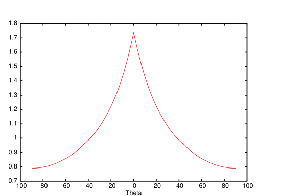
Figure 1: The function $p^{v}_{2}(\theta)$.

We now turn to the simulations to test conjecture (12). We use the pivot algorithm to generate walks in the full plane with a constant number of steps $N$. We take $N=1,000,000$. The lattice spacing and $N$ are such that the size of the SAW is large compared to the domain $D$ so that the SAW is effectively infinite. We condition on the event that the SAW intersects the boundary of $D$ exactly once. The probability of this event goes so zero in the scaling limit, so we must generate very large numbers of SAW’s to get good statistics. We use Clisby’s fast implementation of the pivot algorithm using binary trees [2].

In our first test we take the domain for the cut-curve ensemble to be a disc centered at $0$ where the SAW starts. We take the lattice spacing to be $N^{-\nu}$ and take the radius of the disc to be $R=0.2$. (With $R=0.3$ the effect of the finite length of the SAW begins to be noticeable. At $R=0.4$ it is quite noticeable.) In the simulation we sample the Markov chain every $1000$ iterations and generate a total of approximately $47$ million samples. Just over $10\%$ of these samples satisfy the condition that the SAW only intersects the boundary of the circle once, and we have approximately $4.9$ million samples of the boundary density.

In this geometry both $\rho_{D}(z)$ and $\rho^{*}_{D}(z)$ are constant, so the prediction for the boundary density without lattice effects is just the uniform density. The angle $\theta(z,D)$ of the tangent line at $z$ is equal to the polar angle $\theta$ of $z$ mod $90$ degrees. So if we think of the boundary density as a function of the polar angle $\theta$, then our conjecture (12) is that the boundary density is proportional to $l_{2}(\theta)$. Figure 2 shows the function $l_{2}(\theta)$ and the boundary density we find in the simulation of the cut-curve ensemble. Both functions have a period of $90$ degrees. We plot the boundary density as a function of $\theta$ mod $90$. Both curves are normalized so that the total area under the curves is one.

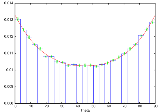
Figure 2: The function $l_{2}(\theta)$ (red curve) and the density for the full plane SAW conditioned to hit a circle exactly once (blue histogram). Note that the range of the vertical axis does not start at $0$.

Figure 2 compares densities. Actually, the function plotted for the simulation of the cut-curve ensemble is a histogram. So the points plotted correspond to the average value of the density over a small interval. The simulations do not compute densities directly. Finding the density requires taking a numerical derivative, i.e., computing a histogram. We can avoid this extra source of numerical error by working with cumulative distribution functions (cdf’s) rather than densities.

In figure 3 we study the cdf for the cut-curve ensemble using the unit disc centered at $0$. We plot two curves. One is the cdf we find in the simulation of the cut-curve ensemble minus the cdf for the uniform density, i.e., the density given by (7). (In this figure we have again taken advantage of the periodicity of the underlying density functions.) This difference is small with the maximum being slightly less than $2\%$, but it is clearly not zero. In the second curve we show the cdf for the simulation of the cut-curve ensemble minus the cdf corresponding to the density given by (12), i.e., corresponding to $l_{2}(\theta)$. The difference is on the order of $0.02\%$. The error bars in the figure are two standard deviations for the statistical errors, i.e., the error that comes from not running the Monte Carlo simulation forever. There are also errors in the simulation from two other sources - the finite length of the SAW and the nonzero lattice spacing. We have studied the error from the finite length of the SAW by simulating the ensemble with several values of the radius of the disc. With $R=0.2$ we believe that the error from the finite length of the SAW is much smaller than the statistical errors. The nonzero lattice spacing means that all our random variables are at a small scale discrete random variables. This is reflected in the slightly jagged nature of the second curve. The error from the nonzero lattice spacing appears to be comparable in size to the statistical error. Thus the difference between the cdf from the simulation and the cdf given by (12) is zero within the errors in our simulation. Figure 3 gives evidence that there are indeed lattice effects that must be taken into account in the boundary density and that our conjecture correctly accounts for these lattice effects.

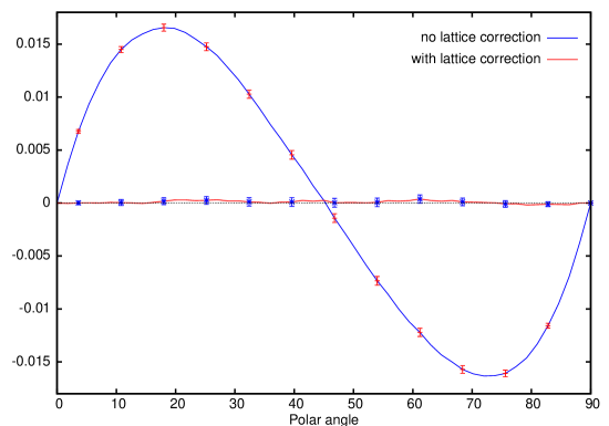
Figure 3: The simulation of the cdf for the boundary density for the cut-curve ensemble for the first geometry minus the theoretical prediction. The larger curve does not include the lattice correction function; the smaller curve does.

For our second test of conjecture (12), we consider the SAW in the upper half plane, starting at the origin. We take the cut-curve to be a semi-circle centered at the origin. Again, we take the lattice spacing to be $N^{-\nu}$ and the radius of the semi-circle disc to be $R=0.2$. We sample the Markov chain every $1000$ iterations and generate a total of approximately $27$ million samples. Approximately $13\%$ of these samples satisfy the condition that the SAW only intersects the boundary of the circle once, and we have approximately $3.6$ million samples of the boundary density for this geometry.

The ensemble consists of all SAW’s in the upper half plane which start at $0$ and only cross the semicircle once. In this geometry the arc length along the semicircle equals the polar angle $\theta$. So we will express densities as functions of $\theta$. A simple computation using the conformal map $z+1/z$ shows that the interior density $\rho_{D}(\theta)$ is $[\sin(\theta)]^{5/8}$. The exterior density $\rho_{D}^{*}(\theta)$ is exactly the same. (This is just a consequence of the symmetry of our geometry under the inversion $z\rightarrow-1/z$.) So our conjecture for the density along the cut-curve is proportional to

$$[\sin(\theta)]^{5/4}\,\,l(\theta)$$ (14)

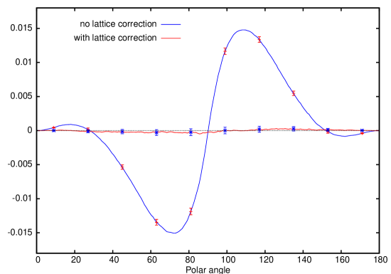
Figure 4: The simulation of the cdf for the boundary density for the cut-curve ensemble for the second geometry minus the theoretical prediction. The larger curve does not include the lattice correction function; the smaller curve does.

The comparison of our simulation of the cut-curve ensemble cdf for the SAW and our conjecture is shown in figure 4. Again we plot two curves. For one curve we find the cdf corresponding to just the density function $[\sin(\theta)]^{5/4}$. This would be the conjectured cdf if there were no lattice effects. We plot the cdf for the simulation of the cut-curve ensemble minus the cdf corresponding to just $[\sin(\theta)]^{5/4}$. This difference is small (the max is on the order of $1.5\%$), but is clearly not zero. For the other curve we compute the cdf corresponding to our conjecture (14) with the lattice effect and subtract this function from the simulation of the cdf for the cut-curve ensemble. The difference is on the order of $0.05\%$ which is zero within the errors in our simulation. This figure gives further evidence that there are indeed lattice effects that must be taken into account in the boundary density and that our conjecture correctly accounts for these lattice effects.

4 Conclusions and future work

We have considered the ensemble of SAW’s in a simply connected domain containing the origin which start at the origin and end on the boundary. It has been noted before that the conjecture for this boundary density will have lattice effects that persist in the scaling limit. We have conjectured that this lattice effect is given by multiplying the density by a function $l(\theta(z,D))$ where $\theta(z,D)$ is the angle of the tangent line to the boundary of $D$ at the point $z\in\partial D$. The lattice correction function $l(\theta)$ depends on the lattice and on how we interpret “ending on the boundary of $D$.” We have shown how to compute the lattice correction function $l(\theta)$ for two particular interpretations. Our focus has been on the distribution of the endpoint of the SAW on the boundary, but we should remark that in light of (4) the lattice effects in this boundary density will produce lattice effects in the probability measure ${\bf P}_{D}$. We have also extended this conjecture to the $\lambda$-SAW.

As we have noted before, there is no efficient way to simulate the natural interpretations of the ensemble of SAW’s in a domain which start at an interior point and end on the boundary. We have circumvented this difficulty by introducing the cut-curve ensemble which can be thought of as an ensemble of two SAW’s, one from the interior point to the boundary and the other from that boundary point to $\infty$. There is another ensemble that is amenable to efficient simulation which is studied in [5]. Given a domain $D$ containing the origin the ensemble is defined as follows. We assume the domain has the property that a ray from the origin only intersects the boundary of the domain in one point. For a SAW $\omega$ we let $\lambda(\omega)>0$ be such that the endpoint of $\omega$ is on the boundary of $\lambda(\omega)D$. In general the SAW need not be inside the dilated domain $\lambda(\omega)D$. Our ensemble consists of all SAW’s $\omega$ of any length such that $\omega$ is contained in $\lambda(\omega)D$. (One must introduce cutoffs to make this a finite measure.) In [5] we show how one can simulate this ensemble using the ensemble of SAW’s of a fixed length.

Finally, it is natural to ask if there is an interpretation of “ending on the boundary of $D$” for which there are no lattice effects in the scaling limit. We speculate that the following ensemble has this property. As before, let $\delta$ be the lattice spacing. Let $\epsilon>0$ and consider all SAW’s that start at the origin, stay inside $D$ and end within a distance $\epsilon$ of the boundary of $D$. We let $\delta$ go to $0$ first and then let $\epsilon$ go to zero. We conjecture that $l(\theta)$ is constant for this ensemble. Unfortunately, the double limit involved in this ensemble makes it difficult to simulate this ensemble.

References

- [1] T. Alberts, H. Duminil-Copin, Bridge decomposition of restriction measures, J. Stat. Phys. 140, 467-493 (2010). Archived as arXiv:0909.0203v1 [math.PR].
- [2] N. Clisby, Efficient implementation of the pivot algorithm for self-avoiding walks, J. Stat. Phys. 140, 349-392 (2010). Archived as arXiv:1005.1444v1 [cond-mat.stat-mech].
- [3] B. Dyhr, M. Gilbert, T. Kennedy, G. Lawler, S. Passon, The self-avoiding walk spanning a strip, J. Stat. Phys. 144, 1–22 (2011).
- [4] H. Duminil-Copin,S. Smirnov, The connective constant of the honeycomb lattice equals . Preprint, 2010. Archived arXiv:1007.0575v1 [math-ph].
- [5] T. Kennedy, in preparation.
- [6] M. Kozdron, G. Lawler, The configurational measure on mutually avoiding SLE paths in Universality and Renormalization: From Stochastic Evolution to Renormalization of Quantum Fields, I. Binder, D. Kreimer, ed., Amer. Math. Soc. (2007).
- [7] G. Lawler, Partition functions, loop measure, and versions of SLE. J. Stat. Phys. 134, 813–837 (2009).
- [8] G. Lawler, V. Limic, Random Walk: A Modern Introduction, Cambridge Univ. Press (2010).
- [9] G. Lawler, Schramm-Loewner evolution, in Statistical Mechanics, S. Sheffield and T. Spencer, ed., IAS/Park City Mathematical Series, AMS, 231-295 (2009). Archived as arXiv:0712.3256v1 [math.PR].
- [10] G. Lawler, O. Schramm, and W. Werner, On the scaling limit of planar self-avoiding walk, Fractal Geometry and Applications: a Jubilee of Benoit Mandelbrot, Part 2, 339–364, Proc. Sympos. Pure Math. 72, Amer. Math. Soc., Providence, RI, 2004. Archived as arXiv:math/0204277v2 [math.PR]
- [11] G. Lawler, W. Werner (2004), The Brownian loop soup, Probab. Theory Related Fields 128, 565–588.
- [12] P. Lévy, Processus Stochastiques et Mouvement Brownien, Gauthiers-Villars, Paris (1946).
- [13] N. Madras and G. Slade, The Self-Avoiding Walk. Birkhäuser (1996).
- [14] B. Nienhuis, Exact critical exponents for the models in two dimensions, Phys. Rev. Lett. 49 1062-1065 (1982).
- [15] F. and M. Riesz, Über die Randwerte einer analytischen Funktion, Quatrième Congrès des Mathématiciens Scandinaves, Stockholm, pp. 27-44 (1916).