On the fibration of augmented link complements

Abstract.

We study the fibration of augmented link complements. Given the diagram of an augmented link we associate a spanning surface and a graph. We then show that this surface is a fiber for the link complement if and only if the associated graph is a tree. We further show that fibration is preserved under Dehn filling on certain components of these links. This last result is then used to prove that within a very large class of links, called locally alternating augmented links, every link is fibered.

1. Introduction

Let $K$ be an oriented link in $S^{3}$. By a Seifert surface $S$ we mean an orientable spanning surface for $K$, i.e., $\partial S=K$ and the orientation of $S$ agrees with that of $K$. It is known that every oriented link has a Seifert surface (see for instance [17]). We say the link $K$ is fibered if $S^{3}-K$ has the structure of a surface bundle over the circle, i.e., if there exists a Seifert surface $S$ such that $S^{3}-K\cong(S\times[0,1])/\phi$, where $\phi$ is a homeomorphism of $S$. In this case we abuse terminology and say $S$ is a fiber for $K$.

The study of the fibration of link complements has been an active line of research in low dimensional topology. In [11] Harer showed how to construct all fibered knots and links. However, deciding whether or not a link $K$ is fibered is in general a very hard problem. Stallings [18] proved that a link $K$ is fibered if and only if $\pi_{1}(S^{3}-K)$ contains a finitely generated normal subgroup whose quotient is $\mathbb{Z}$. Stallings’ result is very general, but hard to verify, even if we restrict to particular families of links. In the early 60’s Murasugi [14] proved that an alternating link is fibered if and only if its reduced Alexander polynomial is monic. In [8] Gabai proved that if a Seifert surface $S$ can be decomposed as the Murasugi sum of surfaces $S_{1},...,S_{n}$, then $S$ is a fiber if and only if each of the surfaces $S_{i}$ is a fiber (refer to theorem 4). Melvin and Morton [13] studied the fibration of genus 2 knots. Goodman–Tavares [10] showed that under simple conditions imposed on certain spanning surfaces, it is possible to decide whether or not these surfaces are fibers for pretzel links. Their method is very algebraic and relies on Stallings’ work [18]. Very recently Futer–Kalfagianni–Purcell ([6], theorem 5.11) introduced a new method for deciding whether or not a given spanning surface is fiber for a link $K$. From a diagram of the link they construct an associated surface (called the $A$-state surface) and a certain graph. They show that this surface is a fiber if and only if the corresponding graph is a tree. Later, Futer [4] extended this result to a larger class of links (homogeneous links) using combinatorial arguments.

In this paper we will be mainly concerned with the fibration of three classes of links: augmented links, locally alternating augmented links, and links obtained from augmented links by Dehn filling on certain components. Given the diagram of an augmented link we associate a spanning surface and a graph. We then show that this surface is a fiber for the link complement if and only if the associated graph is a tree. We also show that when this is the case, then Dehn filling on certain components of these links produces fibered manifolds. This last result is then used to show that every locally alternating augmented link is fibered, and explicitly exhibit their fibers. A relevant remark here is that the surfaces and graphs we consider are very different from those in [6] and [4]. It is also interesting to observe that we obtain the same type of results: a link complement is fibered if and only if an associated graph is a tree.

The relevance of studying augmented links is that they have played a central role in several recent developments in 3-manifold topology. Lackenby and Agol–Thurston [12] used them to estimate volumes of alternating link complements. Futer–Kalfagianni–Purcell [5] used them to obtain diagrammatic volume estimates of many knots and links. Futer–Purcell [7] also used them to prove that if $K$ is a link with a twist-reduced diagram with at least 4 twist regions and at least 6 crossings per twist region, then every non-trivial Dehn filling on $K$ is hyperbolic. Their combinatorial argument further implies that every link with at least 2 twist regions and at least 6 crossings per twist region is hyperbolic and gives a lower bound for the genus of $K$. Cheesebro–DeBlois–Wilton [3] proved that hyperbolic augmented links satisfy the virtual fibering conjecture.

We next define the classes we will be working with and state the main results.

2. Augmented links, locally alternating augmented links and main results

The notion of augmented links was first introduced by Adams [1] and further explored by Futer–Kalfagianni–Purcell [5], Futer–Purcell [7] and Purcell [16]. We recall it here. For more details see the very nice survey paper on augmented links by Purcell [15].

Let $K$ be a link in $S^{3}$ with diagram $D(K)$. Regard $D(K)$ as a $4$-valent graph in the plane. A bigon region is a complementary region of the graph having two vertices in its boundary. A string of bigon regions of the complement of this graph arranged end to end is called a twist region. A vertex adjacent to no bigons will also be a twist region. Encircle each twist region with a single unknotted component, called a crossing circle, obtaining a link $J$. $S^{3}-J$ is homeomorphic to the complement of the link $L$ obtained from $J$ by removing all full twists from each twist region. The link $L$ is called the augmented link associated to $D(K)$. The original link complement can be obtained from the link $L$ by performing $1/n$-Dehn filling on the crossing circles, for appropriate choices of $n$.

Figure 1. (a) Initial link $K$; (b) link $J$ obtained by adding crossing circles; (c) augmented link $L$; (d) corresponding flat augmented link.

When all the twist regions in the diagram $D(K)$ have an even number of crossings, then all non-crossing circle components of the augmented link $L$ will be embedded in the projection plane. We call these links flat augmented links.

Given the diagram of a flat augmented link $L$ we construct a Seifert surface $S_{L}$, called standard Seifert surface, and a graph $G_{B}(L)$ (this will be done in section 4). We now state our main results.

Theorem 1.

Let $L$ be a flat augmented link. Then the standard Seifert surface $S_{L}$ is a fiber if and only if the graph $G_{B}(L)$ is a tree.

Performing $\pm 1$ Dehn filling on crossing circle components of links as above yield new ones which are again fibered.

Theorem 2.

Let $L$ be an flat augmented link such that the graph $G_{B}(L)$ is a tree. Then $\pm 1$ Dehn filling on crossing circle components yields a fibered link $K$.

Given a flat augmented link $L$, one can construct a corresponding locally alternating augmented link $L_{a}$ as follows: in each crossing circle change two of the crossings so that the crossings in the crossing circles are alternating. This is described in Figure 2. Note that the resulting link need not to be alternating.

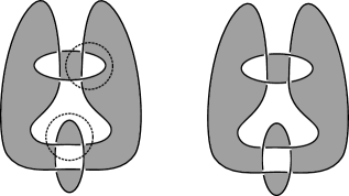
Figure 2. Left: Pairs of crossings yielding locally alternating link; Right: Seifert surface for resulting link.

We later show that every locally alternating augmented link $L_{a}$ can be obtained from $\pm 1$ filling on the crossing circles of a flat augmented link $\tilde{L}$ such that $G_{B}(\tilde{L})$ is a tree. This implies

Theorem 3.

Let $L_{a}$ be a locally alternating augmented link obtained from a flat augmented link $L$ with a connected diagram. Then $L_{a}$ fibers.

Remark 1.

We remark that our methods and the surfaces and graphs we construct are very different from those in [6] or even [4]. However, it is very interesting that we are obtaining the same type of results: a manifold fibers given that a certain associated graph is a tree. We also note that very often fibration of the links considered here cannot be detected from their construction but is detected by ours (examples for the converse can also be exhibited).

The remainder of the paper is organized as follows: in section 3 we we recall the notion of Murasugi sum. This will be used in the decomposition of the standard surface. In section 4 we set up the terminology of standard surface and of the graph $G_{B}(L)$ needed for the remainder of the paper. In section 5 we prove theorem 1. In section 6 we prove theorem 2 . Finally, in section 7 we use theorem 2 to prove theorem 3.

3. Murasugi Sum

In this section we recall the notion of Murasugi sum ([9] and [14]).

Definition 1.

We say that the oriented surface $T$ in $S^{3}$ is with boundary $L$ is the Murasugi sum of the two oriented surfaces $T_{1}$ and $T_{2}$ with boundaries $L_{1}$ and $L_{2}$ if there exists a $2$-sphere $S$ in $S^{3}$ bounding balls $B_{1}$ and $B_{2}$ with $T_{i}\subset B_{i}$ for $i=1,2$, such that $T=T_{1}\cup T_{2}$ and $T_{1}\cap T_{2}=D$ where $D$ is a $2n$-sided disk contained in $S$ (see Figure 3).

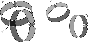
Figure 3. Murasugi sum of two Hopf bands

The result concerning Murasugi sum we need is the following, due to Gabai [8].

Theorem 4 (Gabai).

Let $T\subset S^{3}$, with $\partial T=L$, be a Murasugi sum of oriented surfaces $T_{i}\subset S^{3}$, with $\partial T_{i}=L_{i}$, for $i=1,2$. Then $S^{3}-L$ is fibered with fiber $T$ if and only if $S^{3}-L_{i}$ is fibered with fiber $T_{i}$ for $i=1,2$.

Remark 2.

We abuse notation by saying that $L$ is the Murasugi sum of $L_{1}$ and $L_{2}$.

4. Set up

The augmented links we consider are flat, i.e., there are no twists adjacent to crossing circles. Our goal is to find a condition under which such links fiber. Recall that Stallings [18] provided a method for checking whether or not a given Seifert surface is a fiber for the complement of an oriented link.

Theorem 5 (Stallings).

Let $T\subset S^{3}$ be a compact, connected, oriented surface with nonempty boundary $\partial T$. Let $T\times[-1,1]$ be a regular neighborhood of $T$ and let $T^{+}=T\times\{1\}\subset S^{3}-T$. Let $f=\varphi|_{T}$, where $\varphi:T\times[-1,1]\longrightarrow T^{+}$ is the projection map. Then $T$ is a fiber for the link $\partial T$ if and only if the induced map $f_{*}:\pi_{1}(T)\longrightarrow\pi_{1}(S^{3}-T)$ is an isomorphism.

Consider the diagram of $L$ as a planar graph. This graph divides the plane into regions which are checkerboard colored. The unbounded region is colored white and the other regions are colored accordingly. Black regions correspond to a Seifert surface, called standard surface, which induces an orientation on the link $L$. This surface will be denoted $S_{L}$. There are three types of white regions:

• Type $A$ regions, bounded by crossing circles that bound two white regions;

• Type $B$ regions, bounded by crossing circles that bound a single white region;

• Type $C$ regions, not bounded by crossing circles.

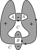
Figure 4. Standard Seifert surface for augmented link and corresponding white regions determined by the diagram

Note that type $A$ regions come in pairs. We will the denote the above regions by $A_{11},A_{12},A_{21},A_{22},...,A_{p1},A_{p2},B_{1},...,B_{q},C_{1},...,C_{r}$ respectively. We denote the unbounded white region by $C_{0}$.

A crossing circle bounding a type $B$ region $B_{i}$ will be called a $B$-circle, also denoted by $B_{i}$. Note that given the diagram for $L$, as described above, there will be two type $C$ regions adjacent to each $B$-circle. A crossing circle bounding a pair of type $A$ regions $A_{i1},A_{i2}$ will be called a $A$-circle and denoted by $A_{i}$. Note that there will be two type $C$ regions adjacent to each $A$-circle. Let $G_{B}(L)$ be the graph obtained from the diagram of $L$ as follows (see figure 5).

• Vertices are type $C$ regions;

• An edge joins $C_{i}$ and $C_{j}$ if there is a $B$-circle adjacent to them.

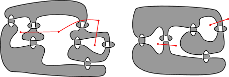
Figure 5. Left: Graph $G_{B}(L)$ associated to the standard surface is a tree; Right: $G_{B}(L)$ is disconnected.

The standard surface $S_{L}$ can be obtained as the Murasugi sum of a surface $S_{L^{\prime}}$ and a collection of Hopf bands. We can remove each $A$-circle in the diagram by deplumbing (i.e., undoing Murasugi sum) a pair of Hopf bands. This is described in figure 6. Applying this procedure to every $A$-circle we obtain a new augmented link $L^{\prime}$, with standard surface $S_{L^{\prime}}$. This decomposition will be used in the proof of theorem 1.

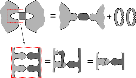
Figure 6. Decomposing a pair of Hopf bands for each $A$-circle.

5. Proof of theorem 1

Theorem 1.

Let $L$ be a flat augmented link. Then the standard Seifert surface $S_{L}$ is a fiber if and only if the graph $G_{B}(L)$ is a tree.

The standard surface $S_{L}$ is obtained as the Murasugi sum of a collection of Hopf bands together with the surface $S_{L^{\prime}}$. Each of these Hopf bands is a fiber for the complement of their boundary Hopf links. The link $L^{\prime}$ is the boundary of $S_{L^{\prime}}$. $L^{\prime}$ is itself a flat augmented link in which all crossing circles are $B$-circles. The surface $S_{L^{\prime}}$ is two-sided (i.e., orientable): from above the diagram we see the “$-$”side of the surface on the black regions bounded by $B$-circles. The other black regions represent the “$+$”side. We use this orientation throughout the paper.

Observe that, by construction, $G_{B}(L)=G_{B}(L^{\prime})$. In view of Theorem 4 we need to find conditions under which the surface $S_{L^{\prime}}$ is a fiber for the link $L^{\prime}$. This is given by the following.

Lemma 6.

The oriented link $L^{\prime}$ fibers with fiber $S_{L^{\prime}}$ if and only if its associated graph $G_{B}(L^{\prime})$ is a tree.

This lemma concludes the proof of Theorem 1.

Figure 7. Surfaces $S_{L^{\prime}}$ obtained from the standard surfaces in figure 5

.

We now proceed to prove the lemma.

Proof.

First observe that the link $L^{\prime}$ is itself a flat augmented link, obtained from $L$ by decomposing a pair of Hopf bands for each $A$-circle. The diagram of $L^{\prime}$ divides the plane into type $B$ and type $C$ regions.

Observe also that the fundamental group of the surface $S_{L^{\prime}}$ is free. Let $B_{1},...,B_{q}$ and $C_{1},...,C_{r}$ be the type $B$ and $C$ regions given by the diagram of $L^{\prime}$. A generating set for $\pi_{1}(S_{L^{\prime}})$ is given as follows. Consider simple closed curves on $S_{L^{\prime}}$ around these regions. They are labeled $\alpha_{b_{1}},...\alpha_{b_{q}},\alpha_{c_{1}},...,\alpha_{c_{r}}$ and are oriented in the counter-clockwise direction. Now choose a base point $a\in S_{L^{\prime}}$ in such a way that, when seen from above the projecting plane, it lies in the “$+$”side of $S_{L^{\prime}}$. Finally, add arcs $h_{b_{1}},...,h_{b_{q}},h_{c_{1}},...,h_{c_{r}}$ from $a$ to each of the curves above. This gives loops $\beta_{b_{i}}=h_{b_{i}}\alpha_{b_{i}}h_{b_{i}}^{-1}$, $\beta_{c_{j}}=h_{c_{j}}\alpha_{c_{j}}h_{c_{j}}^{-1}$ based at $a$. This set of based loops corresponds to a generating set for $\pi_{1}(S_{L^{\prime}})$. These generators will be denoted by $u_{b_{1}},...,u_{b_{q}}$, $u_{c_{1}},...,u_{c_{r}}$.

The fundamental group of the complement $S^{3}-S_{L^{\prime}}$ is also free. We now describe a generating set for this group. As before, let $C_{0}$ denote the unbounded white region determined by the diagram of $L^{\prime}$. Let $B_{i}$ denote a white region determined by a $B$ circle and let $\gamma_{b_{i}}\subset S^{3}-S_{L^{\prime}}$ be a semicircle with one endpoint in $C_{0}$ and the other in $B_{i}$, lying under the projecting plane. Associated to each $B$ region we construct a simple closed curve by connecting the endpoints of the arc $\gamma_{b_{i}}$ to the point $f(a)$ by straight line segments. Here, $a$ is the base point for $\pi_{1}(S_{L^{\prime}})$ and $f:S_{L^{\prime}}\longrightarrow S^{3}-S_{L^{\prime}}$ is described in theorem 5. Each of these curves is oriented so that, starting at $f(a)$, we move along the line segment connecting $f(a)$ to the endpoint of $\gamma_{b_{i}}$ in $B_{i}$, then move along $\gamma_{b_{i}}$ to the second endpoint and then back to $f(a)$ through the second line segment. Make a similar construction for each type $C$ region. We have built loops with base point $f(a)$ corresponding to a set of generators for $\pi_{1}(S^{3}-S_{L^{\prime}})$. These generators are denoted by $x_{b_{1}},...,x_{b_{q}},x_{c_{1}},...,x_{c_{r}}$, according to the type of region they cross.

We can now describe the induced map $f_{*}$ in terms of these generators. If $\beta$ is a loop in $S_{L^{\prime}}$ based at $a$ then $f(\beta)$ is a loop in $S^{3}-S_{L^{\prime}}$ based at $f(a)$. If $u\in\pi_{1}(S_{L^{\prime}})$ represents the homotopy class of $\beta$, then $f_{*}(u)$ is an element in $\pi_{1}(S^{3}-S_{L^{\prime}})$ given as a word in the letters $x_{b_{1}},...,x_{b_{q}},x_{c_{1}},...,x_{c_{r}}$ as follows: start at $f(a)$ and move along $f(\beta)$. If it crosses a white region other than $C_{0}$ from above to below the projecting plane, we write the corresponding letter $x\in\{x_{b_{1}},...,x_{b_{q}},x_{c_{1}},...,x_{c_{r}}\}$. If it crosses the white region from below to above the projecting plane, we write the letter $x^{-1}$. If it crosses $C_{0}$ we do not write any letters. Going around $f(\beta)$ once gives the desired word.

Now let $\beta_{b_{1}},...,\beta_{b_{q}},\beta_{c_{1}},...,\beta_{c_{r}}$ be the based loops corresponding to the generators of $\pi_{1}(S_{L^{\prime}})$ as above. They were given by $\beta_{b_{i}}=h_{b_{i}}\alpha_{b_{i}}h_{b_{i}}^{-1}$, $\beta_{c_{j}}=h_{c_{j}}\alpha_{c_{j}}h_{c_{j}}^{-1}$.

Let $B_{i},C_{n},C_{m}$ be white regions, $C_{n},C_{m}$ adjacent to the $B$-circle $B_{i}$, as in figure 8. The loops in figure 8 (left) represent the simple closed curves in $S_{L^{\prime}}$ around these regions. There, we indicate the corresponding generators of $\pi_{1}(S_{L^{\prime}})$. Their images under $f_{*}$ are given by

$$\left\{\begin{array}[]{lr}u_{b_{i}}\mapsto g_{b_{i}}x_{c_{m}}x_{c_{n}}^{-1}g_{b_{i}}^{-1}\\ u_{c_{m}}\mapsto g_{c_{m}}x_{b_{i}}x_{c_{m}}^{-1}w_{m}g_{c_{m}}^{-1},\hskip 5.69046pt\text{$w_{m}$ is a word without the letter $x_{b_{i}}$};\\ u_{c_{n}}\mapsto g_{c_{n}}x_{c_{n}}x_{b_{i}}^{-1}w_{n}g_{c_{n}}^{-1},\hskip 5.69046pt\text{$w_{n}$ is a word without the letter $x_{b_{i}}$}.\end{array}\right\}$$

Here $g_{b_{i}},g_{c_{j}}$ are the words we get in the letters $\{x_{b_{1}},...,x_{b_{q}},x_{c_{1}},...,x_{c_{r}}\}$ by moving along the arcs $h_{b_{i}},h_{c_{j}}$ respectively. Thus, up to conjugation, we get

(1) $$\left\{\begin{array}[]{lr}u_{b_{i}}\mapsto x_{c_{m}}x_{c_{n}}^{-1}\\ u_{c_{m}}\mapsto x_{b_{i}}x_{c_{m}}^{-1}w_{m},\hskip 5.69046pt\text{$w_{m}$ is a word without the letter $x_{b_{i}}$};\\ u_{c_{n}}\mapsto x_{c_{n}}x_{b_{i}}^{-1}w_{n},\hskip 5.69046pt\text{$w_{n}$ is a word without the letter $x_{b_{i}}$}.\end{array}\right\}$$

Remark 3.

• If a $B$-circle is adjacent to the unbounded region $C_{0}$ and another region $C_{m}$, then, up to conjugation, we have $u_{b_{i}}\mapsto x_{c_{m}}^{\pm 1}$.

• We may assume the words $w_{m},w_{n}$ do not have the letter $x_{b_{i}}$. If they did, this would imply the simple closed curves $\alpha_{c_{m}},\alpha_{c_{n}}$ around $C_{m}$ and $C_{n}$ are the same curve, which would mean $C_{m}$ and $C_{n}$ represent the same region. In this case the circle $B_{i}$ would not be linked to the other components of $L^{\prime}$, i.e., $L^{\prime}$ would be a split link, which is not fibered.

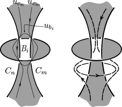
Figure 8. Left: Loops around white regions corresponding to generators $u_{b_{i}},u_{c_{m}}$ and $u_{c_{n}}$; Right: Their images under $f$.

The strategy now is as follows: by theorem 5 $S_{L^{\prime}}$ is a fiber if and only if the map $f_{*}:\pi_{1}(S_{L^{\prime}})\longrightarrow\pi_{1}(S^{3}-S_{L^{\prime}})$ is an isomorphism. We show that if $G_{B}(L^{\prime})$ is not a tree then the map induced by $f_{*}$ on homology is not an isomorphism. Therefore $f_{*}$ cannot be isomorphism. When $G_{B}(L^{\prime})$ is a tree we prove that $f_{*}$ is surjective. Since free groups have the Hopfian property, it follows that $f_{*}$ is an isomorphism.

First assume $G_{B}(L^{\prime})$ is not a tree

Consider the map $\bar{f}_{*}:H_{1}(S_{L^{\prime}})\longrightarrow H_{1}(S^{3}-S_{L^{\prime}})$ induced on homology by $f_{*}$. Denote by $\bar{u}_{b_{1}},...,\bar{u}_{b_{q}}$, $\bar{u}_{c_{1}},...,\bar{u}_{c_{r}}$ the generators of $H_{1}(S_{L^{\prime}})$, corresponding to the above generators of $\pi_{1}(S_{L^{\prime}})$. The generators of $H_{1}(S^{3}-S_{L^{\prime}})$ are constructed similarly and denoted $\bar{x}_{b_{1}},...,\bar{x}_{b_{q}}$, $\bar{x}_{c_{1}},...,\bar{x}_{c_{r}}$.

Case 1. $G_{B}(L^{\prime})$ has two or more connected components:

Let $C_{1},...,C_{n+1}$ represent the vertices of a component not containing the vertex $C_{0}$. Let $\beta\subset S_{L^{\prime}}$ be a simple closed curve around the regions $C_{1},...,C_{n+1}$. This loop is obviously non-trivial in $S_{L^{\prime}}$. Moreover, the corresponding element $\bar{u}\in H_{1}(S_{L^{\prime}})$ is also non-trivial. However we see that $f(\beta)$ is a trivial loop in $S^{3}-S_{L^{\prime}}$ and therefore $\bar{f}_{*}(\bar{u})\in H_{1}(S^{3}-S_{L^{\prime}})$ is trivial.

Case 2. $G_{B}(L^{\prime})$ contains a non-trivial loop: Let $C_{1},...,C_{n},C_{n+1}=C_{1}$ represent the vertices and $B_{1},...,B_{n}$ the edges of this loop. In (1) above we have expressions for $f_{*}$ up to conjugation. Therefore, at the level of homology, we have

$$\bar{f}_{*}(\bar{u}_{b_{i}})=-\bar{x}_{c_{i}}+\bar{x}_{c_{i+1}}$$

and thus

$$\bar{f}_{*}(\bar{u}_{b_{1}}+\cdots+\bar{u}_{b_{n}})=(-\bar{x}_{c_{1}}+\bar{x}_{c_{2}})+\cdots+(-\bar{x}_{c_{n}}+\bar{x}_{c_{1}})=0$$

The same argument holds if the loop contains the vertex corresponding to $C_{0}$.

Suppose now $G_{B}(L^{\prime})$ is a tree. In this case note that there is only one “+”region seen from above the projecting plane. We take the base point $a\in S_{L^{\prime}}$ lying in this region. This choice of base point allows us to choose the arcs $h_{b_{i}},h_{c_{j}}$ in $S_{L^{\prime}}$ joining $a$ to the simple closed curves around the white regions in such a way that all these arcs lie in the “+”region of $S_{L^{\prime}}$. In this situation, the expressions in (1) give the actual images under $f_{*}$ of the generators of $\pi_{1}(S_{L^{\prime}})$. We now show $f_{*}$ is surjective.

Step 1.

Let $C_{0}$ be the initial vertex and let $C_{1},...,C_{k}$ be the vertices connected to $C_{0}$ by edges represented by the $B$-circles $B_{1},...,B_{k}$. We have

$$u_{b_{i}}\mapsto x_{c_{i}}^{\pm 1}$$

Thus $x_{c_{i}}$ is the image of either $u_{b_{i}}$ or $u_{b_{i}}^{-1}$.

Step 2.

Let $C_{11},...,C_{1k_{1}}$ be connected to $C_{1}$ by edges $B_{11},...,B_{1k_{1}}$. Note that, since $G_{B}(L^{\prime})$ is a tree, $C_{1i}\neq C_{j}$ for $i=1,...,k_{1}$ and $j=0,...,k$. We thus have

$$u_{b_{1j}}\mapsto x_{c_{1}}^{\pm 1}x_{c_{1j}}^{\mp 1}$$

And hence

$$u_{b_{1}}^{\mp 1}u_{b_{1j}}\mapsto x_{c_{1j}}^{\mp 1}$$

This determines preimages for $x_{c_{1i}}$ in terms of $u_{b_{1i}}$ and $u_{b_{1}}$.

Step 3.

Repeat Step 2 for $C_{2},...,C_{k}$. These $C_{i}$’s are the ones defined in Step 1. This determines preimages for $x_{c_{ji}}$ in terms of $u_{b_{ji}}$ and $u_{b_{j}}$.

Step 4.

Inductively find preimages for all the $x_{c}^{\prime}s$ in terms of the $u_{b}^{\prime}s$. Note that, for this step to work, it is necessary that $G_{B}(L^{\prime})$ is a tree.

Now we need to find preimages for the $x_{b}$’s.

Step 5.

From

$$u_{c_{m}}\mapsto x_{c_{m}}^{-1}x_{b_{i}}w_{m},\text{$w_{m}$ word without the $x_{b_{i}}$ letter}$$

$$u_{c_{n}}\mapsto x_{c_{n}}x_{b_{i}}^{-1}w_{n},\text{ $w_{n}$ word without the $x_{b_{i}}$ letter}$$

we show how to obtain the $x_{b}$’s as images of $u_{b}$’s and $u_{c}$’s.

Since $G_{B}(L^{\prime})$ is a tree, each $C$-region corresponding to a terminal vertex is adjacent to a single $B$-circle. Suppose $C_{m}$ is such a region. In this case we have $u_{c_{m}}\mapsto x_{c_{m}}^{-1}x_{b_{i}}$ and thus we obtain $x_{b_{i}}$ as the image of a word in the letters $u_{b}^{\prime}s$ and $u_{c}^{\prime}s$ (and their inverses). Repeat this process for all the terminal vertices. Inductively we can find all the $x_{b}$’s as the image of a word in the letters $u_{b}$’s and $u_{c}$’s. ∎

6. Dehn filling on crossing circles

In this section we prove

Theorem 2.

Let $L$ be an flat augmented link such that the graph $G_{B}(L)$ is a tree. Then $\pm 1$ Dehn filling on crossing circle components yields a fibered link $K$.

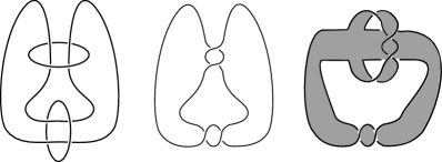
Figure 9. Left: Original link; Center: $\pm 1$ filling on crossing circles; Right: Standard Seifert surface for resulting link.

Proof.

$\pm 1$ filling on a $A$-circles yields a fibered link. To see this consider the link $L^{\prime}$ constructed as in the last section. Recall that when $L$ fibers with fiber $S_{L}$, then $L^{\prime}$ fibers with fiber $S_{L^{\prime}}$. $A$-circles in $L$ correspond to the Murasugi sum of two Hopf bands with $L^{\prime}$. It should be easy to see that $\pm 1$ filling on a $A$-circle corresponds to the sum of a single Hopf band (see figure 9). Therefore, by theorem 4, the statement is true for filling on $A$-circles.

The proof of the statement for $B$-circles is similar to the proof that $S_{L^{\prime}}$ is a fiber for $L^{\prime}$. Let $K^{\prime}$ be the link obtained from $L^{\prime}$ by performing $\pm 1$ Dehn filling on the $B$-circles. We consider the standard Seifert surface $S_{K^{\prime}}$ obtained from the Seifert algorithm applied to the link $K^{\prime}$ (see Figure 10). This surface is the surface obtained by checkerboard coloring the regions determined by the diagram of $K^{\prime}$ in the projecting plane (this is a 4-valent diagram). We now describe the map $f_{*}:\pi_{1}(S_{K^{\prime}})\longrightarrow\pi_{1}(S^{3}-S_{K^{\prime}})$. First we introduce some conventions. We may consider the simple closed curves around white regions of $S_{K^{\prime}}$, oriented counter-clockwise. As before, since $G_{B}(L)$ is a tree, we only see a single “+”region on $S_{K^{\prime}}$. Take a base point $a\in S_{K}^{\prime}$ in this region and add an arc from this base point to each of the simple closed curves. We have built a set of based loops corresponding to generators for $\pi_{1}(S_{K^{\prime}})$. Denote this set by $\{u_{c}\}$. Similar to the construction in section 5, we have a corresponding set of generators $\{x_{c}\}$ for $\pi_{1}(S^{3}-S_{K^{\prime}})$. We see that we may associate to $S_{K^{\prime}}$ a tree $G_{B}(K^{\prime})$ identical to $G_{B}(L^{\prime})$. Vertices correspond to white regions and two vertices are joined by an edge if they are adjacent to a pair of crossings obtained by filling on a $B$-circle (see Figure 10). The node of the tree is the vertex corresponding to the unbounded region $C_{0}$. We say this vertex is at level $0$. Let $C_{11},...C_{1s}$ be the vertices adjacent to $C_{0}$. We say these edges are at level $1$. Recursively define vertices at higher levels. $f_{*}$ is described as follows:

Figure 10. Left: link $L^{\prime}$; Right: $K^{\prime}$ and its standard Seifert surface.

• For a terminal vertex, say $C_{m}$, on $G_{B}(K^{\prime})$ we have: $u_{c_{m}}\mapsto w=x_{c_{m}}x_{c_{m-1}}^{-1}$ or $u_{c_{m}}\mapsto w^{\prime}=x_{c_{m-1}}x_{c_{m}}^{-1}$, where $C_{m-1}$ is the vertex one level lower than $C_{m}$ and adjacent to it.

• Let $C_{1}$ be a vertex at level 1 (adjacent to $C_{0}$). Suppose $C_{1}$ is also a terminal vertex. We have $u_{c_{1}}\mapsto x_{c_{1}}^{\pm 1}$.

• If $C_{1}$ is not a terminal vertex, let $C_{21},\cdots,C_{2s}$ be the vertices at level 2 adjacent to it. We have $u_{c_{1}}\mapsto x_{c_{1}}^{\pm 1}w_{1}w_{2}\cdots w_{s}$, where the $w_{i}$ are of one the forms $w_{i}=x_{c_{2i}}x_{c_{1}}^{-1}$ or $w_{i}=x_{c_{1}}x_{c_{2i}}^{-1}$.

• An intermediate vertex (not a terminal vertex nor adjacent to $C_{0}$) $C_{k-1}$, say at level $k-1$, is adjacent to vertices $C_{k1},\cdots,C_{ks}$ at level $k$ and to a single vertex $C_{k-2}$ at level $k-2$. We have $u_{c_{k-1}}\mapsto(x_{c_{k-1}}x_{c_{k-2}}^{-1})^{\pm 1}w_{1}w_{2}\cdots w_{s}$, where the $w_{i}$ are of one the forms $w_{i}=x_{c_{k-1}}x_{c_{ki}}^{-1}$ or $w_{i}=x_{c_{ki}}x_{c_{k-1}}^{-1}$.

The set of generators for the free group $\pi_{1}(S_{K^{\prime}})$ is $\{u_{c_{ij}}\}$ and the set of generators for $\pi_{1}(S^{3}-S_{K^{\prime}})$ is $\{x_{c_{ij}}\}$. Note that $f_{*}$ maps the set $\{u_{c_{ij}}\}_{c}$ to $\{y_{ij}\}$, where $y_{ij}$ is a word on the letters $x_{c_{ij}}$. Given the tree structure on $G_{B}(K^{\prime})$ and the description of $f_{*}$ above, it is not very hard to see how to obtain $\{y_{ij}\}$ from $\{x_{c_{ij}}\}_{c}$ by a sequence of Nielsen transformations (see example below): start at a terminal vertex $C_{m}$ and replace $x_{c_{m}}$ by $y_{m}$, where $y_{m}=x_{c_{m}}x_{c_{m-1}}^{-1}$ or $y_{m}=x_{c_{m-1}}x_{c_{m}}^{-1}$. Repeat this for all terminal vertices. Using the description of $f_{*}$ as above and an inductive argument (part 3 in the description of $f_{*}$ above) we see how to obtain all the $y_{ij}$ by a sequence of Nielsen transformations. Therefore the map $f_{*}:\pi_{1}(S_{K^{\prime}})\longrightarrow\pi_{1}(S^{3}-S_{K^{\prime}})$ is an isomorphism. ∎

Example 1.

For the example in Figure 10 we have:

$$u_{c_{11}}\mapsto x_{c_{11}},u_{c_{12}}\mapsto x_{c_{12}}x_{c_{2}}x_{c_{12}}^{-1},u_{c_{2}}\mapsto x_{c_{12}}x_{c_{2}}^{-1}$$

and the sequence of Nielsen transformations is given by

$\begin{cases}x_{c_{11}}\mapsto x_{c_{11}}&\mapsto x_{c_{11}}\\ x_{c_{12}}\mapsto x_{c_{12}}&\mapsto x_{c_{12}}(x_{c_{12}}x_{c_{2}}^{-1})^{-1}\\ x_{c_{2}}\mapsto x_{c_{12}}x_{c_{2}}^{-1}&\mapsto x_{c_{12}}x_{c_{2}}^{-1}\\ \end{cases}$

7. Locally alternating augmented links

Given a flat augmented link $L$, we construct a corresponding locally alternating augmented link $L_{a}$ as described in section 2 (see Figure 2). Regarding the fibration of the oriented link $L_{a}$, we get a stronger statement.

Theorem 3.

Let $L_{a}$ be a locally alternating augmented link obtained from a flat augmented link $L$ with a connected diagram. Then $L_{a}$ fibers.

This theorem follows immediately from

Lemma 7.

Let $L_{a}$ be a locally alternating augmented link obtained from a flat augmented link $L$ with a connected diagram. Then $L_{a}$ is obtained from $\pm 1$ Dehn filling on the crossing circles of a flat augmented link $\tilde{L}$ such that $G_{B}(\tilde{L})$ is a tree.

Proof.

Just as for $L$, construct the standard Seifert surface for $L_{a}$, as well as the corresponding graph $G_{B}(L_{a})$. Given $L_{a}$, suppose $G_{B}(L_{a})$ is not a tree.

Step 1.

Eliminate nontrivial loops in $G_{B}(L_{a})$ :

Choose a loop $\gamma$ in $G_{B}(L_{a})$ and an edge $e$ on this loop (a $B$-circle on $L_{a}$) connecting vertices $v_{1},v_{2}$ corresponding to regions $C_{1},C_{2}$. Figure 11 shows how to obtain $L_{a}$ from $\pm 1$ filling on a $A$-circle of a new link $L_{a1}$. The relationship between $G_{B}(L_{a})$ and $G_{B}(L_{a_{1}})$ is that $G_{B}(L_{a1})$ is obtained from $G_{B}(L_{a})$ by adding a new vertex $v_{3}$ in the interior of $e$ and breaking the loop $\gamma$ at $v_{3}$.

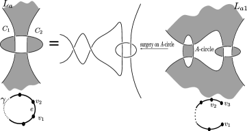
Figure 11. Removing the loop $\gamma$ from $G_{B}(L_{a})$.

Step 2.

Join disconnected components of $G_{B}(L_{a})$:

Consider two vertices $v_{1},v_{2}$ on $G_{B}(L_{a})$ not in the same component but such that their corresponding $C$-regions $C_{1},C_{2}$ are adjacent to a $A$-circle. Figure 12 shows how to obtain $L_{a}$ from $\pm 1$ filling on a $B$-circle of a new link $L_{a2}$. The relationship here is that $G_{B}(L_{a2})$ is obtained from $G_{B}(L_{a})$ by joining $v_{1},v_{2}$ by a new edge $e$.

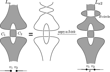
Figure 12. Joining vertices $v_{1}$ and $v_{2}$.

Step 3.

Repeat the steps above, as needed, until we obtain a link $\tilde{L}_{0}$ such that $G_{B}(\tilde{L}_{0})$ is a tree. Note that some of its crossing circles are alternating and some are not. $L_{a}$ is obtained from $\tilde{L}_{0}$ by a sequence of $\pm 1$ fillings on its flat crossing circles (these ones are the ones introduced in the steps above).

The conclusion now follows from the observation that alternating crossing circles can be obtained from $\pm 1$ filling on a pair of flat crossing circles, as described in Figure 13. The desired link $\tilde{L}$ is the link obtained from $\tilde{L}_{0}$ by replacing alternating crossing circles by a pair of non-alternating ones. Note that since $G_{B}(\tilde{L}_{0})$ is a tree, $G_{B}(\tilde{L})$ is also a tree. ∎

Figure 13. Obtaining alternating crossing circles from fillings on non-alternating ones.

References

- [1] C. Adams, Augmented alternating link complements are hyperbolic, Low-dimensional topology and Kleinian groups(Coventry-Durham, 1984), London Math. Soc. Lecture Notes Ser., vol. 112, Cambridge Univ. Press, Cambridge, 1986, pp. 115–130.
- [2] C. Adams, Thrice-punctured spheres in hyperbolic 3-manifolds, Trans. Am. Math. Soc., Vol 287(1985), 645–656
- [3] J.DeBlois, E. Chesebro, H. Wilton, Some virtually special hyperbolic 3-manifold groups, Commentarii Mathematici Helvetici, 87(3), pp. 727-–787, 2012.
- [4] D. Futer, Fiber detection for state surfaces, preprint
- [5] D. Futer, E. Kalfagianni, J. Purcell, Dehn filling, volume and the Jones polynomial, Journal of Differential Geometry, Vol. 78 (2008), no. 3, 429–464.
- [6] D. Futer, E. Kalfagianni, J. Purcell, Guts of surfaces and the colored Jones polynomial, Monograph to appear in Lecture Notes in Mathematics (Springer), volume 2069.
- [7] D. Futer, J. Purcell, Links with no exceptional surgeries,Commentarii Mathematici Helvetici, Vol. 8 (2007), no. 3, 629–664.
- [8] D. Gabai, Detecting fibred links in , Comment. Math. Helvetici 61 (1986) 519–555
- [9] D. Gabai, The Murasugi sum is a natural geometric operation II, Comtemporary Mathematics, 20 (1983), 131–143.
- [10] S. Goodman, G. Tavares, Pretzel-fibered links, Bol. Soc. Bras. Mat., vol 15, ’s 1 e 2 (1984), 85–96
- [11] J. Harer, How to construct all fibered knots and links, Topology 21 (1982) 263–280.
- [12] M. Lackenby, The volume of hyperbolic alternating link complements. With an appendix by Ian Agol and Dylan Thurston, Proc. London Math. Soc. 88 (2004) 204–224.
- [13] P. M. Melvin, H. R. Morton, Fibred knots of genus 2 formed by plumbing Hopf bands, J. London Math. Soc. (2) 34 (1986) 159–168.
- [14] K. Murasugi, On a certain subgroup of the group of an alternating link, Amer. J. of Math. 85, (1963), 544–550.
- [15] J. Purcell, An introduction to fully augmented links, Interactions between hyperbolic geometry, quantum topology, and number theory, Contemporary Mathematics, Vol 541, (2011), pp. 205–220.
- [16] J. Purcell, Volumes of highly twisted knots and links, Algebraic & Geometric Topology, Vol. 7 (2007), pp. 93–108.
- [17] D. Rolfsen, Knots and links, AMS Chelsea Publishing, Dec. 2003.
- [18] J. Stallings, On fibering of certain 3-manifolds Topology of 3-manifolds and related topics, Prentice-Hall, Englewood Cliffs, N.J., 1962