Oscillations of networks: the role of soft nodes

Abstract

To describe the flow of a miscible quantity on a network, we consider the graph wave equation where the standard continuous Laplacian is replaced by the graph Laplacian. The structure of the graph influences strongly the dynamics which is naturally described using the eigenvectors as a basis. Assuming the graph is forced and damped at specific nodes, we derive the amplitude equations. These reveal the importance of a soft node where the eigenvector is zero. For example forcing the network at a resonant frequency reveals that damping can be ineffective if applied to such a soft node, leading to a disastrous resonance and destruction of the network. We give sufficient conditions for the existence of soft nodes and show that these exist for general graphs so that they can be expected for complex physical networks and engineering networks like power grids.

¹:Laboratoire de Mathématiques, INSA de Rouen,
B.P. 8, 76131 Mont-Saint-Aignan cedex, France
E-mail: caputo@insa-rouen.fr
²: Physics Department,
Faculty of Sciences, University of Yaounde I,
B. P. 812 Yaounde - Cameroon

1 Introduction

The flow of a scalar quantity in a network is an important problem for fundamental science and engineering applications. The latter include gas, water or power distribution networks. Other examples are a simplified version of road traffic and the flow of nerve impulse in the brain. The static aspect of the problem has long been studied within the framework of operations research, see for example [1]. However in many cases the dynamic character is crucial. Take for example the prediction of traffic jams in a given road network or the prediction of a flood in a river basin.

The basic equations describing the flow of a miscible quantity are the well-known conservation laws of mathematical physics. These laws are building blocks for studying physical systems. They are universal and can be found for example in mechanics and in electromagnetism. Each conservation law has the form of a flux relation

$$u_{t}+\partial_{x}q=0,$$ (1)

where the first term is the time derivative of a density $u$ and the second one is the space derivative of the flux $q$ along the relevant coordinate. The most important conserved quantities in mechanics are the mass, momentum and energy. In electromagnetism the current and voltage obey conservation laws.

To describe the flow of a given quantity on a network it is natural to generalize these conservation laws. For that one uses the graph representing the network. The derivative is now the generalized gradient $\nabla$ or its transpose, the incidence matrix. To write this, it is important to orient the branches of the graph. In the static regime, these equations are usually solved as an optimization problem, see [4] for an example of a gas network. The dynamic problem is solved numerically using ordinary differential equation solvers. In general, it is difficult to analyze the problem. There are however, classes of systems which can be analyzed. This happens when dissipation exists only at the nodes and not on the branches. A typical example is a small power grid where the power line dissipation can be neglected and where only power input and output occur at given nodes. If the system is linear and possesses some symmetry, the equations can be reduced to a graph wave equation as named by Friedman and Tillich [2]. There, the usual Laplacian is replaced by its discrete analog, the graph Laplacian $\nabla^{T}\nabla$. The graph wave equation was studied by Maas [3] who considered graphs obtained by linking elementary graphs. He established particular inequalities for the first non zero eigenvalue of the Laplacian of these graphs. The graph Laplacian was also considered recently by Burioni et al for the thermodynamics of the Hubbard model to describe static configurations of a Josephson junction array [5]. Another problem considered by that group is to use the graph as a controlled obstacle to obtain a desired reflection of discrete nonlinear Schrödinger solitons [6].

In this article we adopt a more applied point of view. We recall how conservation laws lead to the graph wave equation. This is illustrated in three different physical contexts: a network of inductances and capacities, its equivalent mechanical analog represented by masses and springs and an array of fluid ducts. From another point of view, the graph wave equation can describe small oscillations of a network near its functioning point. The key point is that all nodes have the same inertia in the dynamics. Then the formulation using the graph wave equation is very useful because the graph Laplacian i.e. the spatial part of the equation is a symmetric matrix so that its eigenvalues are real and its eigenvectors are orthogonal. It is then natural to describe the dynamics of the network by projecting it on a basis of the eigenvectors. We consider that the network is fixed and is submitted to forcing and damping on specific nodes and obtain the new amplitude equations. These reveal that when a component of an eigenvector for a mode is zero the forcing or damping is ineffective. This concept of a ”soft node” is formalized. We then show what are the sufficient conditions for general graphs to present such soft nodes. The numerical analysis of a network forced close to resonance confirms the initial observation. When the network is damped on a soft node, the damping is ineffective. This can have catastrophic consequences because the amplitude of the oscillations increases without bounds. Another notable effect occurs when a multiple eigenvalue corresponds to different eigenvectors. Then depending how the system is excited we get a different response. These are effects that can occur for a general network and can have important practical consequences.
The article is organized as follows, section 2 presents the derivation of the graph wave equation in different physical contexts. In section 3 we formalize the notion of ”soft node” and give sufficient conditions for a graph to have one. The amplitude equations are analyzed numerically in section 5. There we force the simple graphs of section 3 at resonance and analyze their response. We conclude in section 6.

2 The model: graph wave equation

We now introduce the basic notions from graph theory following the presentation of [7]. A graph ${\cal G}(N,B)$ is the association of a node set $N$ and a branch set $B$ where a branch is an unordered pair of distinct nodes. We assume that the nodes and branches are numbered $N=\{1,2,\dots n\}$ and $B=\{1,2,\dots m\}$ and that $n>1$ and $m>0$. The vertices are oriented with an arbitrary but fixed orientation. We consider for simplicity only simple graphs which do not have multiple branches. In the following we will refer to Fig. 1 shows such a graph with $n=4$ nodes and $m=3$ branches.

Figure 1: Schematic drawing of the complex graph oscillator. The arrows on the branches are oriented arbitrarily.

The basic tool for expressing a flux is the so-called incidence matrix $A(n,m)$ defined as

$$A_{nb}=-1~{}~{}{\rm~{}if~{}branch}~{}b~{}{\rm starts~{}from~{}node~{}}n,$$ (2)

$$A_{nb}=1~{}~{}{\rm~{}if~{}branch}~{}b~{}{\rm finishes~{}at~{}node~{}}n,$$ (3)

$$A_{nb}=0{\rm~{}otherwise}$$ (4)

In this section we present the conservation laws and derive the graph wave equation using as example the graph of Fig. 1. This is done for pedagogical reasons so the article is easier to read for non specialists. All these results can be easily generalized to any graph. For the example shown in Fig. 1, we have

$$A=\left(\begin{matrix}-1&0&0\cr 1&-1&-1\cr 0&1&0\cr 0&0&1\end{matrix}\right)$$

The transpose $A^{T}=\nabla$ is a discrete differential operator ( gradient of graph). To see this consider a function $f:N\to R$. The vector $\nabla f$ has as $b$ component the difference of the values of $f$ at the end points of the branch $b$ (with orientation). In the example above, we have

$$\nabla f=\left(\begin{matrix}-1&1&0&0\cr 0&-1&1&0\cr 0&-1&0&1\end{matrix}\right)\left(\begin{matrix}f_{1}\cr f_{2}\cr f_{3}\cr f_{4}\end{matrix}\right)=\left(\begin{matrix}f_{2}-f_{1}\cr f_{3}-f_{2}\cr f_{4}-f_{2}\end{matrix}\right),$$ (5)

which is the discrete gradient of $f$ associated to the graph.

We now consider different networks where this formalism applies. We will first write conservation laws using the $\nabla$ operator or its transpose. From there we establish the relevant wave equation. These derivations are shown for the example of Fig. 1 for pedagogical reasons, they can be generalized to any graph. For the specific inductance-capacity electrical network shown in the left panel of Fig. 2, the equations of motion in terms of the (node) voltages and (branch) currents are the conservation of current and voltage

$$Cv_{t}-\nabla^{T}i=s,$$ (6)

$$Li_{t}-\nabla v=0,$$

where

$$C=\left(\begin{matrix}C_{1}&0&0&0\cr 0&C_{2}&0&0\cr 0&0&C_{3}&0\cr 0&0&0&C_{4}\end{matrix}\right),~{}~{}~{}L=\left(\begin{matrix}L_{1}&0&0\cr 0&L_{2}&0\cr 0&0&L_{3}\end{matrix}\right)~{},$$

are respectively the diagonal matrix of capacities and the diagonal matrix of inductances and $s$ represents the currents applied to each node. (similar to boundary conditions in the continuum case). Note that the equations (6) also describe in the linear limit, shallow water waves in a network of canals and fluid flow in a pipe network. In the first situation $v$ corresponds to a surface elevation and $i$ to a flux. For the second example $v$ is the pressure and $i$ the flux. From the two equations (6) one obtains the generalized wave equation. For this take the derivative of the 1st equation and substitute the second to obtain the node wave equation

$$Cv_{tt}-\nabla^{T}L^{-1}\nabla v=s_{t},$$ (7)

where

$$\nabla^{T}L^{-1}\nabla=\left(\begin{matrix}L_{1}^{-1}&-L_{1}^{-1}&0&0\cr-L_{1}^{-1}&L_{1}^{-1}+L_{2}^{-1}+L_{3}^{-1}&-L_{2}^{-1}&-L_{3}^{-1}\cr 0&-L_{2}^{-1}&L_{2}^{-1}&0\cr 0&-L_{3}^{-1}&0&L_{3}^{-1}\end{matrix}\right)~{}.$$ (8)

There is a corresponding branch wave equation for the currents that involves the link Laplacian in the terminology of [2]. Taking the time derivative of the second equation and substituting into the first we get

$$Li_{tt}-\nabla C^{-1}\nabla^{T}i=\nabla C^{-1}s.$$ (9)

In the rest of the article we will only consider the node graph wave of the type (7).

A similar graph wave equation arises when describing the other physical system shown in the right panel of Fig. 2, the collection of four masses $m_{i},~{}i=1-4$ connected by springs of stiffnesses $k_{i},~{}i=1-3$. Here the variables are the displacements $y_{i},~{}i=1-4$ of each mass. The equations of motion are

$$\left\{\begin{array}[]{llll}m_{1}\ddot{y_{1}}=k_{1}\left(y_{2}-y_{1}\right)\\ m_{2}\ddot{y_{2}}=k_{1}\left(y_{1}-y_{2}\right)+k_{2}\left(y_{3}-y_{2}\right)+k_{3}\left(y_{4}-y_{2}\right)\\ m_{3}\ddot{y_{3}}=k_{2}\left(y_{2}-y_{3}\right)\\ m_{4}\ddot{y_{4}}=k_{3}\left(y_{2}-y_{4}\right).\\ \end{array}\right.$$

Notice the correspondence capacities / masses and inverse inductances / stiffnesses. The matrix on the right hand side is symmetric just like the matrix in the second term on the left hand side of (7).

Figure 2: Two different physical networks corresponding to the graph shown in Fig. 1. The left panel shows a network of inductances and capacities and the right panel shows the mechanical analog in terms of masses and springs

In the following we will consider the graph shown in Fig. 3 which includes an additional branch between nodes 3 and 4. We assume that the masses are equal. This is important because it preserves the symmetry of the operator. For simplicity we choose $k_{1}=k_{3}=k$, $k_{2}=\alpha^{2}k$ and $k_{4}=\beta^{2}k$.

Figure 3: The specific network that will be studied throughout the article.

Then we normalize times by the natural frequency

$$\omega=\sqrt{\frac{k}{m}},~{}~{}t\prime=\omega t.$$ (10)

Omitting the primes, the equations can be written in matrix form as

$$\left(\begin{array}[]{c}\ddot{y_{1}}\\ \ddot{y_{2}}\\ \ddot{y_{3}}\\ \ddot{y_{4}}\\ \end{array}\right)=\left(\begin{array}[]{cccc}-1&1&0&0\\ 1&-2-\alpha&\alpha&1\\ 0&\alpha&-\alpha-\beta&\beta\\ 0&1&\beta&-1-\beta\\ \end{array}\right)\left(\begin{array}[]{c}y_{1}\\ y_{2}\\ y_{3}\\ y_{4}\\ \end{array}\right),$$ (11)

which we will write formally as

$$Y_{tt}=GY,$$ (12)

where $G$ is the graph Laplacian [7], the equivalent of (8).

Another way of defining the graph Laplacian $G$ is to consider the adjacency matrix $M=(m_{ij})$ where $m_{ij}$ is the weight of the branch connecting node $i$ to node $j$. The weight is zero if the branch is absent. The degree matrix $D=(d_{i})$ is the diagonal matrix such that

$$d_{i}=\sum_{j\neq i}m_{ij}.$$

We then have

$$G=\nabla^{T}\nabla=-D+M.$$ (13)

In the rest of the article we keep the masses the same. Equation (11) in the absence of $\alpha$ and $\beta$ is a finite difference discretisation of the 1D continuous Laplacian. This connects the model with a continuous wave equation. When $\alpha>0$ and $\beta>0$ we have a generalization of this finite difference description. In a way we have a discrete version of coupled wave equations. From another point of view the graph wave equation above describes small oscillations of a general (nonlinear) system around it’s operating state. It is a very general model.

The linear evolution problem (12) gives rise to periodic solutions $Y(t)=Z\exp({i\omega t})$ where the $Z$ verify the spectral problem

$$GZ=-\omega^{2}Z.$$ (14)

The matrix $G$ is symmetric. If we had assumed different masses on the nodes, we would have lost this property. For electrical networks this corresponds to the same capacity in equation (7). This property is important because symmetric matrices have real eigenvalues and we can always build a basis of orthogonal eigenvectors. These eigenvalues are stable with small symmetric perturbations of the network, like for example adding a link. In this sense the eigenmodes are characteristic of the network. The eigenvectors provide a basis of $R^{n}$ which is adapted to describe the evolution of $Y$ on the graph. Specifically we arrange the eigenvalues $\lambda_{i}=-\omega_{i}^{2}$ as

$$|\lambda_{1}|=0\leq|\lambda_{2}|\leq\dots\leq|\lambda_{n}|.$$ (15)

We label the associated eigenvectors $v_{1},v_{2},\dots,v_{n}$. These verify

$$Gv_{i}=-\omega_{i}^{2}v_{i}.$$ (16)

and are orthogonal with respect to the standard scalar product. We then normalize them so $<v_{i},v_{j}>=\delta_{i,j}$ where $\delta_{i,j}$ is the Kronecker symbol. Notice that $G$ is a singular matrix since the sum of its lines (resp. columns) gives a 0 line (resp. column). Therefore $G$ will have a zero eigenvalue which corresponds to the Goldstone mode. The solutions of the linear system $GY=S$ are given up to a constant.

It is natural to write the equation of motion (12) in terms of the amplitudes of the normalized eigenvectors $v_{i},~{}~{}Y=\sum_{i}a_{i}v_{i}$. We obtain the standard result

$${\ddot{a}_{i}}+\omega_{i}^{2}a_{i}=0,$$ (17)

so that the normal modes do not exchange energy. The problem is then Hamiltonian with

$$H={1\over 2}\sum_{i}{\dot{a}_{i}}^{2}+\omega_{i}^{2}{a_{i}}^{2}.$$ (18)

When a perturbation acts on the system the equations need to be modified. This is the object of the next section.

3 Forcing the network : amplitude equations

For a general (nonlinear) evolution problem of the form

$$Y_{tt}=GY+N(Y),$$ (19)

it is natural to expand $Y$ using the eigenvectors as

$$Y(t)=a_{1}(t)v_{1}+a_{2}(t)v_{2}+\dots+a_{n}(t)v_{n}.$$ (20)

Inserting (20) into (19) and projecting on each mode $v_{i}$ we get the system of coupled equations

$${a_{1}}_{tt}+\omega_{1}^{2}a_{1} = <N(Y)|v_{1}>,$$ (21)

$${a_{2}}_{tt}+\omega_{2}^{2}a_{2} = <N(Y)|v_{2}>,$$ (22)

$$\dots$$ (23)

$${a_{n}}_{tt}+\omega_{n}^{2}a_{n} = <N(Y)|v_{n}>.$$ (24)

We expect this decomposition to be more adapted to describe the dynamics of $Y$ on the graph. In particular it should explain some of the unexpected couplings that are observed between the modes.

Let us now assume that the network is forced at some node $n_{f}$ and damped at some node $n_{d}$. The motion can be represented as

$$Y_{tt}=GY+D(-dY_{t})+Ff{\bf 1},$$ (25)

where the $(n,n)$ matrices $D,~{}F$ are everywhere 0 except for $D(n_{d},n_{d})=1,~{}F(n_{f},n_{f})=1$ and where $d$ is a damping coefficient and $f$ a forcing coefficient. The vector ${\bf 1}$ is ${\bf 1}=(1,1,\dots,1)^{T}$. Assuming the linear combination for $Y$ (20) and projecting we get

$$\ddot{a}_{j}=-\omega_{j}^{2}a_{j}-d\sum_{k=1}^{n}<Dv_{k}|v_{j}>{\dot{a}_{k}}+f<F{\bf 1}|v_{j}>.$$ (26)

In terms of components we obtain

$$\ddot{a}_{j}=-\omega_{j}^{2}a_{j}-dv_{j}^{n_{d}}\sum_{k=1}^{n}v_{k}^{n_{d}}{\dot{a}_{k}}+fv_{j}^{n_{f}},~{}~{}j=1,n$$ (27)

where $v_{j}^{n_{d}},~{}v_{j}^{n_{f}}$ are respectively the $n_{d},~{}n_{f}$ components of the normal vector $v_{j}$. From these equations one can see that exciting one node will cause disturbances to propagate all through the network in a precise way. The forcing (resp. the damping) will act on mode $j$ only if the $v_{j}^{n_{f}}\neq 0$ (resp. $v_{j}^{n_{d}}\neq 0$). This important fact leads to the introduction of the concept of ”soft node” which we formalize in the next section.

4 Soft nodes

We introduce the following definitions of a soft node for an eigenmode $j$ of the graph Laplacian $G$.

Definition 4.1 (Soft node )

A node $s$ of a graph is a soft node for an eigenvalue $\lambda$ if there exists an eigenvector $x$ for this eigenvalue such that $x_{s}=0$.

Another definition is the one of absolute soft node.

Definition 4.2 (Absolute soft node )

A node $s$ of a graph is an absolute soft node for an eigenvalue $\lambda$ if every eigenvector $x$ for this eigenvalue is such that $x_{s}=0$.

Note that for single eigenvalues, a soft node is an absolute soft node.

Then we have the following property due to the relation (13)

$$\sum_{i\in\Gamma(s)}m_{is}x_{i}=(deg(s)+\lambda)x_{s},$$ (28)

where $deg(s)=\sum_{i\in\Gamma(s)}m_{is}$ where $\Gamma(s)$ is the set of nodes neighbors to $s$. From this we deduce the following

Proposition 4.3

A soft node $s$ of a graph is such that $\sum_{i\in\Gamma(s)}m_{is}x_{i}=0$.

As illustration consider the graph shown in Fig. 3 with $\beta=0$ and where $\alpha$ is a parameter. This graph is then a tree. The eigenvalues and eigenvectors can be computed analytically, they are given in Table 1 in terms of $\alpha$ and

$$\delta=\sqrt{4\alpha^{2}-4\alpha+9}.$$

index $i$	1	2	3	4
$\lambda_{i}=-\omega_{i}^{2}$	0	-1	${1\over 2}(\delta-2\alpha-3)$	$-{1\over 2}(\delta+2\alpha+3)$
	1	1	1	1
$v_{i}$	1	0	${1\over 2}(\delta-2\alpha-1)$	$-{1\over 2}(\delta+2\alpha+1)$
	1	0	$-{1\over 2}(\delta-2\alpha+3)$	${1\over 2}(\delta+2\alpha-3)$
	1	-1	1	1

Table 1: Eigenmodes $(\lambda_{i},v_{i})$ for the tree.

The frequencies $\omega_{i}=\sqrt{-\lambda_{i}}$ are plotted as a function of the parameter $\alpha$ in Fig. 4. Note how the eigenvalue $\omega_{2}=1$ is independent of $\alpha$. This is because the graph has a swivel at node $3$ as we will explain below. Table 1 shows that $s=2$ and $s=3$ are absolute soft nodes for $\lambda=-1$ and $\alpha\neq 1$. When $\alpha=1$ the eigenvalue $\lambda=-1$ is degenerate and two eigenvectors are $(1,0,0,-1)$ and $(1,0,-2,1)$. The node $s=2$ remains an absolute soft node while the node $s=3$ is soft.

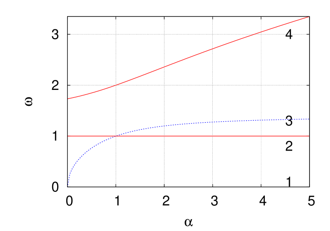
Figure 4: Plot of the eigenfrequencies $\omega_{i},~{}i=1-4$ as a function of $\alpha$ for the graph shown in Fig. 3 with $\beta=0$ i.e. a tree.

The mode $v_{2}$ which is independent of $\alpha$ is shown schematically in Fig. 5 where we have plotted the magnitude and sign of the coordinate using vertical arrows. The arrows are opposite and equal for $v_{2}^{1}$ and $v_{2}^{4}$ because the nodes 1 and 4 play a symmetric role i.e. the graph is invariant by the automorphism transforming node 1 to node 4 [8]. This representation of the eigenmodes is intuitive and gives a direct information on the coupling of the node to the eigenmode. We will use this representation throughout the article.

Figure 5: Schematic representation of the constant mode $v_{2}$, corresponding to $\omega_{2}=1$

.

Let us now consider the other two modes $v_{3}$ and $v_{4}$ which are dependant on $\alpha$. Fig. 6 shows the plots of the components $v_{3}^{i}$ and $v_{4}^{i}$. For $\alpha=1$ we see that the node $s=2$ is soft for the mode $v_{3}$. We will see below that this feature enables to set the functioning point of the network. For $\alpha>5$ the magnitude of $v_{4}^{1}$ and $v_{4}^{4}$ is much smaller than the magnitude of $v_{4}^{2}$ and $v_{4}^{3}$ so that the nodes 4 and 1 are close to soft. Notice how nodes 2 and 3 are soft for $v_{2}$ while nodes 1 and 4 are soft for $v_{4}$ when $\alpha>>1$. Anticipating on the dynamics, one sees that for such large values of $\alpha$, when the graph is forced at a frequency $\omega\approx 1$ the links 1 and 3 will be active and the nodes 2 and 3 will be soft. On the contrary if the graph is forced at a high frequency $\omega\approx\omega_{4}$ only link 2 will be active and nodes 1 and 4 will be soft.

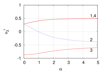
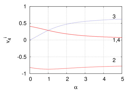
Figure 6: Plot of the components of the non trivial normalized eigenvectors $v_{3}$ (left panel) and $v_{4}$ (right panel) as a function of $\alpha$. soft node for $\alpha=1$ and $v_{3}$

   

   

   

Figure 7: Schematic representation of the non trivial eigenvectors $v_{3},v_{4}$ shown respectively on the left and the right panels. The top panel is for $\alpha=0.1$. It shows the modes $v_{3}$ corresponding to $\omega_{3}=0.36$ (left) and $v_{4}$ corresponding to $\omega_{4}=1.75$ (right). The middle panel is for $\alpha=0.9$ and shows the modes $v_{3}$ corresponding to $\omega_{3}=0.964$ (left) and $v_{4}$ corresponding to $\omega_{4}=1.9671$ (right). The bottom panel corresponds to $\alpha=5$. It shows the modes $v_{3}$ corresponding to $\omega_{3}=1.335$ (left) and $v_{4}$ (right) corresponding to $\omega_{4}=3.35$.

All this information is summarized in Fig. 7 which show a schematic representation of the non trivial eigenvectors for $\alpha=0.1,~{}0.9$ and 5. One can easily identify the soft nodes. As expected by the graph automorphism the components on nodes 1 and 4 of the modes are equal.

Let us return to the $\alpha$-independent eigenvalue $\lambda_{2}=-1$ and its eigenvector $v_{2}$ with soft nodes 2 and 4. These properties exist for general graph configurations of the swivel type which we define in the next section.

4.1 The swivel : a graph with a soft node

Recall that a leaf is a node connected to only one other node.

Definition 4.4 (A swivel )

Given a graph, a swivel (or swivel node) of order $k$ is a node connected to $k$ leaves with all the same coupling $\alpha$.

We have the following property.

Proposition 4.5

For a graph with a swivel of order 2 and coupling $\alpha$, the Laplacian $G$ has an eigenvalue $\lambda=-\alpha$. The swivel node and the other nodes except the leaves are soft for this eigenvalue.

Proof
We consider the situation shown in Fig. 8 where the outer nodes 1 and 2 are connected to a common node 3 which has $p$ connections to the rest ${\cal G}^{\prime}$ of the graph.

Figure 8: A graph such that two leaves are connected to a swivel (with the same coupling).

Assuming $\lambda$ to be an eigenvalue of $G$ we write the matrix $G-\lambda I$

$$G-\lambda I=\left(\begin{array}[]{ccccccccc}-\alpha-\lambda&0&\alpha&0&\dots&\dots&\dots&\dots&0\\ 0&-\alpha-\lambda&\alpha&0&\dots&\dots&\dots&\dots&0\\ \alpha&\alpha&-p-2\alpha-\lambda&m_{34}&\dots&&&&m_{3n}\\ 0&0&m_{34}&&&&&&\\ |&|&|&&&&&&\\ |&|&|&&&A^{\prime}&&&\\ |&|&|&&&&&&\\ |&|&|&&&&&&\\ 0&0&m_{3n}&&&&&&\end{array}\right),$$ (29)

where the submatrix $A^{\prime}$ corresponds to the subgraph ${\cal G^{\prime}}$ and

$$p=\sum_{k=4}^{n}m_{3k}.$$

It is easy to see that if $\lambda=-\alpha$ then the vector $v_{1}$ of coordinates $(x_{1},x_{2},\dots,x_{n})$ where $x_{1}+x_{2}=0$ and $x_{i}=0,i=3,\dots n$ is an eigenvector because $(G+I)v_{1}=0$. Q.E.D.

We now generalize this result to swivels of order $k>1$. The matrix $G-\lambda I$ now has $k$ lines similar to the third line of (29). Following a similar argument as above it can be shown that

Proposition 4.6

If $k$ leaves of a graph are connected to a common swivel $s$ with the same coupling $\alpha$ then $-\alpha$ is an eigenvalue of multiplicity $k-1$. Except maybe the leaves linked to the swivel, all the nodes are soft for the eigenvalue $-\alpha$. The eigenvectors for this eigenvalue will then be such that

$$\sum_{i\in\Gamma(s)}x_{i}=0,$$

where $\Gamma(s)$ is the set of the nodes adjacent (neighbors) to node $s$.

4.2 The closed swivel : another graph with a soft node

Let us now consider that the branches of an order 2 swivel are connected. Then we talk about a graph with a closed swivel.

Definition 4.7 (A closed swivel )

A graph with a closed swivel is constructed by connecting the two leaves of a swivel of order 2 and coupling $\alpha$ by a branch of coupling $\beta$.

We have the following property for the eigenvalues and associated eigenmode of coordinates $x_{i}$.

Proposition 4.8

Assume a graph with a closed swivel of coupling $\beta$. Then the Laplacian has eigenvalue $-1-2\beta$. For this mode, the swivel is a soft node $x_{3}=0$, $x_{1}=-x_{2}$ and $x_{k}=0,~{}k=4\dots n$.

Note that for $\beta=0$ we recover the result of the previous subsection.

Proof
Following the labeling of the graph presented above and summarized in Fig. 8, we assume that the nodes 1 and 2 are connected by an additional link of coupling $\beta$. The matrix $G-\lambda I$ is then

$$G-\lambda I=\left(\begin{array}[]{ccccccccc}-\alpha-\lambda-\beta&\beta&\alpha&0&\dots&\dots&\dots&\dots&0\\ \beta&-\alpha-\beta-\lambda&\alpha&0&\dots&\dots&\dots&\dots&0\\ \alpha&\alpha&-p-2\alpha-\lambda&m_{34}&\dots&&&&m_{3n}\\ 0&0&m_{34}&&&&&&\\ |&|&|&&&&&&\\ |&|&|&&&A^{\prime}&&&\\ |&|&|&&&&&&\\ |&|&|&&&&&&\\ 0&0&m_{3n}&&&&&&\end{array}\right),$$ (30)

Let us show that $\lambda=-\alpha-2\beta$ is an eigenvalue. The form of the equations leads to assume that $x_{i}=0,i\geq 4$. Then the equations for $x_{1},x_{2},x_{3}$ are

$$\beta x_{1}+\beta x_{2}+\alpha x_{3}=0,$$ (31)

$$\beta x_{1}+\beta x_{2}+\alpha x_{3}=0,$$ (32)

$$\alpha x_{1}+\alpha x_{2}+(-p-2-\lambda)x_{3}=0.$$ (33)

which have as only solutions $x_{1}+x_{2}=0$ and $x_{3}=0$. This proves that $-\alpha-2\beta$ is an eigenvalue of $G$, that the swivel is a soft node $x_{3}=0$ and that the eigenvector is such that $x_{1}+x_{2}=0$ and $x_{i}=0,i\geq 4$. Q.E.D.

A simple closed swivel is the graph shown in (3) where we assume $\alpha=1$ and vary $\beta$. The eigenmodes can be computed analytically. They are presented in table 2.

index $i$	1	2	3	4
$\lambda_{i}=-\omega_{i}^{2}$	0	-1	$-1-2\beta$	$-4$
	1	1	0	1
$v_{i}$	1	0	0	-3
	1	-1/2	1	1
	1	-1/2	-1	1

Table 2: Eigenmodes $(\lambda_{i},v_{i})$ for the graph with $\alpha=1$ and a varying $\beta$.

The eigenfrequencies $\omega_{i}=\sqrt{-\lambda_{i}}$ are shown in Fig. 9 as a function of $\beta$. As expected we find the eigenvalues $-1$ and $-1-2\beta$. Notice how $\lambda=-4$ is an eigenvalue. This is specific to this graph. The introduction of the link with coupling $\beta$ is a way to shift the normal modes of the system. Notice the ”crossing” $\lambda_{3}=\lambda_{4}$ for $\beta=3/2$.

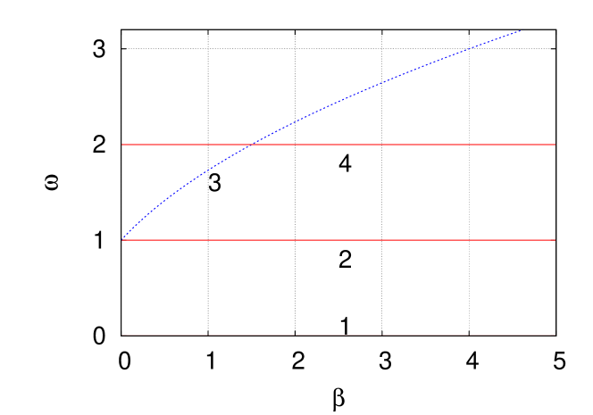
Figure 9: Plot of the eigenfrequencies $\omega_{i},~{}i=1-4$ as a function of $\beta$ for the graph shown in Fig. 3 with $\alpha=1$.

The eigenvectors $v_{2},~{}~{}v_{3}$ and $v_{4}$ are shown respectively from left to right in Fig. 10. Notice how $v_{3}$ corresponding to $\lambda_{3}=-1-2\beta$ is localized on the graph while $v_{2}$ corresponding to $\lambda_{2}=-1$ is not localized.

       

Figure 10: Schematic representation of the eigenvectors $v_{2}$, $v_{3}$ and $v_{4}$ , from left to right

To summarize, we have seen how to generate graphs with soft nodes using swivels. From the amplitude equations we inferred that forcing or damping will not be effective when applied to these soft nodes. In the next section we analyze the dynamics close to resonance when the network is forced or damped at given nodes. We confirm that soft nodes will not be effective.

5 Numerical results: forcing the network

Assume that the graph is forced periodically at a given node $n_{f}$ and damped at a node $n_{d}$, this happening for a time duration $100<t<300$. This forcing and damping is typical for an electrical network. The model can also describe an electrical power grid. The damped nodes correspond to cities where the energy is absorbed and the forced nodes correspond to power stations where energy is introduced in the network. We consider a periodic forcing for simplicity. The result for other types of forcings can be derived from this study using a superposition argument because the system is linear.

The first interesting observation is that damping or driving is ineffective if applied to a soft node. This will happen for any graph, with symmetries or not. The second effect that we will show is when two eigenfrequencies are close. This happens for the tree when $\alpha=1$ or for the graph with a closed swivel when $\beta\approx 0$ or $\beta=3/2$. Some degree of symmetry is usually necessary for this. Then the system can function on two different eigenmodes when it is forced. We will see that the forcing determines which mode is selected.

To illustrate the first effect we choose a tree with $\alpha=0.1,~{}\beta=0$. Fig. 11 shows the different mode amplitudes $a_{i}(t)$ when exciting the tree on node 4 and damping it on node 1 (left panel) and damping it on node 2 (right panel). For the damping on node 1 the corresponding amplitude equations are

$${\ddot{a}_{1}}=d(-0.25{\dot{a}_{1}}-0.15{\dot{a}_{3}}-0.2{\dot{a}_{4}}-0.35{\dot{a}_{2}})+0.5f,$$ (34)

$${\ddot{a}_{2}}+a_{2}=d(-0.35{\dot{a}_{1}}-0.21{\dot{a}_{3}}-0.29{\dot{a}_{4}}-0.5{\dot{a}_{2}})-0.7f,$$ (35)

$${\ddot{a}_{3}}+0.13a_{3}=d(-0.15{\dot{a}_{1}}-0.1{\dot{a}_{3}}-0.12{\dot{a}_{4}}-0.21{\dot{a}_{2}})+0.3f,$$ (36)

$${\ddot{a}_{4}}+3.1a_{4}=d(-0.2{\dot{a}_{1}}-0.12{\dot{a}_{3}}-0.16{\dot{a}_{4}}-0.28{\dot{a}_{2}})+0.4f.$$ (37)

The second equation is resonant if $f=\sin t$ ($\omega=1$ ) but it is damped. This gives rise to an increase of the amplitude of mode 2 with a saturation as shown in the left panel of Fig. 11. The same effect happens if the node 4 is damped. The final value of $a_{2}$ can be obtained by a Green’s function approach. For that we neglect the other modes and write the $a_{2}$ amplitude equation as

$${\ddot{a}_{2}}+\omega_{0}^{2}a_{2}=f(t)-d{\dot{a}_{2}}.$$ (38)

The Green’s function $G(t-t_{0})$ solves

$${\ddot{G}}+\omega_{0}^{2}G+d{\dot{G}}=\delta(t-t_{0}),$$

where $\delta(t-t_{0})$ is the Dirac function at $t_{0}$. From [10] we have

$$G(t-t_{0})=e^{-{d\over 2}(t-t_{0})}{\sin\sqrt{\omega_{0}^{2}-{d^{2}\over 4}}(t-t_{0})\over\sqrt{\omega_{0}^{2}-{d^{2}\over 4}}}.$$ (39)

The solution is then given by

$$a_{2}(t)=\int_{0}^{t}G(t-t_{0})f(t_{0})dt_{0}.$$ (40)

This expression agrees with the plot on the left panel of Fig. 11. When damping is applied to nodes 3 or 4, the equation for $a_{2}$ has no damping, it is

$${\ddot{a}_{2}}+a_{2}=-0.7f.$$ (41)

The amplitude of the mode 2 then grows linearly as expected. This is shown in the right panel of Fig. 11. The final amplitude in Fig. 11 can be easily found by seeing that the solution of the linear resonance equation

$${\ddot{a}_{2}}+a_{2}=f\sin t,$$ (42)

is

$$a_{2}(t)=-{f\over 2}t\cos t.$$ (43)

In the example above one gets

$$max(a_{2}(300))=-{0.7\over 2}(300-100)=70,$$

which is in excellent agreement with the value on the right panel of Fig. 11. This unbounded growth leads to the destruction of the network because damping is ineffective. This will also occur for the graph with a closed swivel damped at node 2 when $\omega\approx\omega_{2}$ or $\omega\approx\omega_{3}$ as shown in Fig. 10. This enumeration shows that this non effectiveness of the damping (or driving) can occur for any network, the only ingredient necessary is the presence of a ”soft node”.

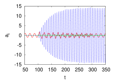
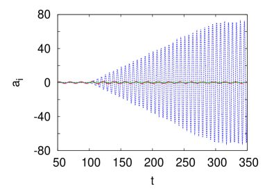
Figure 11: Example of the influence of damping applied to different nodes, the graph is a tree with $\alpha=0.1,~{}\beta=0$. Plot of $a_{2}(t)$ (blue online), $a_{3}(t)$ (red online) and $a_{4}(t)$ (green online) when the node 4 is excited with a frequency $\omega=1$. The left (resp. right) panel corresponds to the node 1 (resp. the node 2) being damped.

Even when the node is close to soft do we get this strong reinforcement of the oscillations. Consider the graph of Fig. 3 with $\beta=\alpha$. It has no particular symmetries and no exact soft nodes. For this more complex graph, the eigenvalues and eigenvectors must be computed numerically. We have used Matlab. The plot of the eigenvalues as a function of $\alpha$ is shown in Fig. 12.

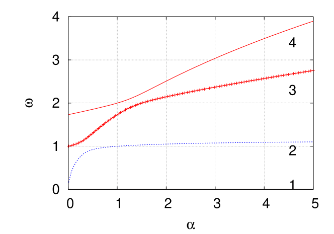
Figure 12: Plot of the eigenfrequencies $\omega_{i},~{}i=1-4$ as a function of $\alpha$ for the graph shown in Fig. 3 with $\alpha=\beta$ i.e. a graph with a cycle.

As expected from the theory [9], the eigenvalues of the graph with a cycle $\mu$ and the eigenvalues of the tree $\lambda$ are interlaced such that

$$0=-\lambda_{1}=-\mu_{1}\leq-\lambda_{2}\leq-\mu_{2}\leq-\lambda_{3}\leq-\mu_{3}\leq-\lambda_{4}\leq-\mu_{4}.$$ (44)

Note that $\lambda_{4}=\mu_{4}$ for $\alpha<1$. The fact that $\lambda_{2}$ and $\lambda_{3}$ are close confines $\mu_{2}$. The dependency of the eigenvectors on the coupling parameter $\alpha$ is shown in Fig. 13.

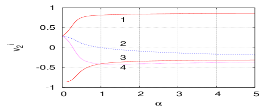
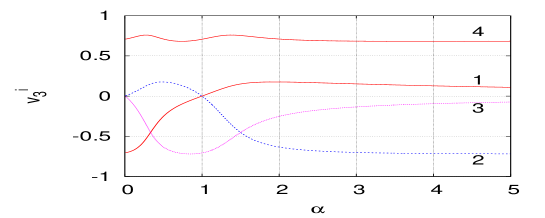
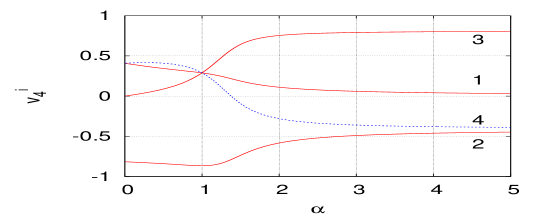
Figure 13: Plot of the components of the non trivial eigenvectors $v_{2},v_{3},v_{4}$ from top to bottom as a function of $\alpha$.

As shown in the middle panel of Fig. 13 for $\alpha=0.1=(\beta)$ and mode 3 node 2 is close to soft while node 1 is non zero. We force the network at frequency $\omega=1\approx\omega_{3}$ to be close to resonance. When the graph has a cycle so that $\alpha=\beta=0.1$ we get a slightly different picture because the linear resonance observed previously is not exact. There is a small damping due to the non zero second coordinate of the eigenvector $v_{3}$. We excite node 4 at a frequency $\omega=1$ and damp the nodes 1,2,3 and 4 respectively. We find two groups of behaviors shown in Fig. 14, the left panel corresponds to damping on nodes 2 and 3. As expected the maximum amplitude of mode $a_{3}$ is much larger than when nodes 1 and 4 are damped (right panel). This is because nodes 2 and 3 are almost soft and not nodes 1 and 4. One can see the typical beat at frequency $(\omega_{3}-\omega)/2$ which yields a half-period $T/2=157$. The mode 2 which is the initial condition is strongly reduced. Note that on the left panel the amplitude of mode 3 is practically constant during and after the forcing/damping region.

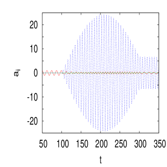
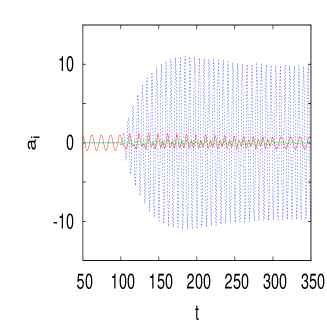
Figure 14: Similar plot as in Fig. 11 except that the graph now has a cycle $\alpha=0.1,~{}\beta=0.1$. Plot of $a_{3}(t)$ (blue online) and $a_{2}(t)$ (red online) when the node 4 is excited with a frequency $\omega=1$. The left (resp. right) panel corresponds to the node 2 (resp. 1) being damped.

This shows that approximate soft nodes exist also in graphs without a particular symmetry. Fig. 13 shows that for large $\alpha$ nodes 1 and 3 are almost soft for $v_{3}$ and node 1 is almost soft for $v_{4}$.

Another effect that occurs in fairly symmetric graphs is that eigenfrequencies can ”cross” as a parameter is varied. This means that two close frequencies can correspond to two eigenmodes that can be very different. If one of the modes has a soft node and the other does not, one can control which mode will appear by selectively exciting or damping a given node of the network. As an example consider the tree graph with $\alpha=0.9,~{}\beta=0$. As shown in Fig. 4 we have two close eigenvalues

$$\omega_{2}=1,~{}v_{2}=\left(\begin{matrix}0.71\cr 0\cr 0\cr-0.71\end{matrix}\right)~{}~{},\omega_{3}=0.964,~{}v_{3}=\left(\begin{matrix}0.4\cr 0.028\cr-0.82\cr 0.4\end{matrix}\right).$$

Mode 2 has $s=2$ and 3 as soft nodes while mode 3 has $s=2$ almost soft. We have excited node 4 with a frequency $\omega=1=\omega_{2}\approx\omega_{3}$. The time evolution of the modes $a_{2}$ and $a_{3}$ are shown in Fig. 15 respectively in light and dark grey (blue and red online).

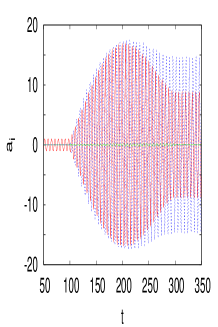
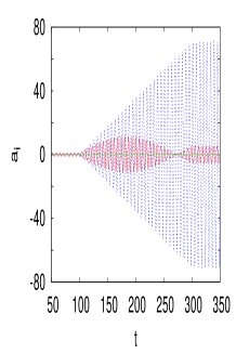
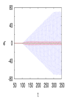
Figure 15: Effect of a multiple eigenvalue in the Laplacian $G$. Plot of $a_{2}(t)$ (blue online) and $a_{3}(t)$ (red online) when the node 4 is excited with a frequency $\omega=1$. The panels correspond respectively to damping the 1st node (left), damping the second node (middle) and damping the 3rd node (right). The parameters are $\alpha=0.9,~{}\beta=0$ and the system is started on the third mode $v_{3}$.

When node 1 is damped, both modes $v_{2}$ and $v_{3}$ can be excited because they have non zero components on that node. This is shown in the left panel of Fig. 15. On the contrary when node 2 is damped (middle panel of Fig. 15) no damping occurs for the amplitude $a_{2}$ causing an unbounded linear growth. The mode $v_{3}$ is excited but in a much smaller way because it is weakly damped, since $v_{3}$ has a small non zero component on node 2. When node 3 is damped (right panel of Fig. 15), the mode 3 is strongly damped so that there is practically only mode 2. Therefore one sees that applying damping to node 3 will result in mode 2 only being excited while applying damping on node 1 will result in the presence of both modes 2 and 3.

6 Conclusion

To describe the flow of a miscible quantity on a network, we considered the graph wave equation where the standard continuous Laplacian is replaced by the graph Laplacian. We have only considered a node wave equation. There would be a similar branch wave equation. We showed that a natural example is an electrical network of inductances on the branches and capacities on the nodes. This system can also describe shallow water waves on a network of canals or fluid flow in a network of pipes. There is also a mechanical analog in terms of masses and springs. In general this graph wave equation describes the small oscillations of a network around it’s functioning point.

Since the graph Laplacian is a symmetric matrix, its eigenvectors can be chosen to be orthogonal. These provide a natural basis to describe the flow in terms of amplitudes on each mode. We derived such amplitude equations when the network is forced and damped on a given node. The eigenvalues and components of the eigenvectors are important elements of these amplitude equations. The amplitude equations revealed the importance of soft nodes where one of the eigenvector components is zero. Any action like forcing or damping on such a node is ineffective. The concept was formalized. We also showed that a sufficient condition for a graph to have a soft node is to have a swivel. Approximate soft nodes can also occur when the couplings depend on a parameter.

The numerical analysis of the amplitude equations when the network is forced at resonance confirmed the importance of soft nodes. In particular if damping is applied to such a node, the network will go into an unbounded resonance which has catastrophic effects. The network can also have multiple eigenvalues. If one of the eigenmodes has a soft node, we showed how the system can be controlled to have one mode only appear or to have two modes appear.

These soft nodes will appear in graphs with symmetries, for example swivels. They can also be found in graphs where the couplings depend on a parameter. This study can then be applied to complex physical networks, like a power grid.

Acknowledgements

The authors thank the Region Haute-Normandie for support through the grant ”Statique et dynamique de réseaux simples” (GRR-TLTI). Elie Simo thanks the Laboratoire de Mathematiques de l’INSA for its hospitality during two visits in 2008 and 2009. The authors thank the Centre de Ressources Informatiques de Haute-Normandie for the use of their computing ressources.

References

- [1] M. Gondran and M. Minoux, ”Graphs and Algorithms”, John Wiley and Sons, (1984).
- [2] J. Friedman and J.-P. Tillich, ”Wave equations for graphs and the edge-based Laplacian”, Pacific J. of Mathematics, vol. 216, nb. 2, (2004).
- [3] C. Maas, ”Transportation in graphs and the admittance sepctrum”, Discrete Applied Mathematics, 16, 32-49, (1987).
- [4] Yue Wu, Kin Keung Lai and Yongjin Liu, ”Deterministic global optimization approach to steady-state distribution gas pipiline networks”, Optim. Eng. 8, 259-275, (2007).
- [5] R. Burioni, D. Cassi, M. Rasetti, P. Sodano and A. Vezzani, ”Bose-Einstein condensation on inhomogeneous complex networks”, J. Phys. B 34, 4697-4710, (2001).
- [6] R. Burioni, D. Cassi, P. Sodano , A. Trombettoni and A. Vezzani, ”Soliton propagation on chains with simple nonlocal defects”, Physica D 216, 71-76, (2006).
- [7] T. Biyikoglu, J. Leydold and P. F. Stadler ”Laplacian Eigenvectors of Graphs”, Springer (2007).
- [8] D. Cvetkovic, P. Rowlinson and S. Simic, ”An Introduction to the Theory of Graph Spectra”, London Mathematical Society Student Texts (No. 75), (2001).
- [9] B. Mohar, ”The Laplacian spectrum of graphs”, in ”Graph Theory, Combinatorics and Applications”, vol. 2 Ed. Y. Alavi G. Chartrand, O. R. Oellermannand A. J. Schwenk, Wiley, (1991).
- [10] R. V. Churchill, Operational mathematics, Mc Graw Hill, (1972).