Filter-design perspective applying to dynamical decoupling of a multi-qubit system

Abstract

We employ the filter-design perspective and derive the filter functions according to nested Uhrig dynamical decoupling (NUDD) and Symmetric dynamical decoupling (SDD) in the pure-dephasing spin-boson model with N qubits. The performances of NUDD and SDD are discussed in detail for a two-qubit system. The analysis shows that (i) SDD outperforms NUDD for the bath with a soft cutoff while NUDD approaches SDD as the cutoff becomes harder; (ii) if the qubits are coupled to a common reservoir, SDD helps to protect the decoherence-free subspace while NUDD destroys it; (iii) when the imperfect control pulses with finite width are considered, NUDD is affected in both the high-fidelity regime and coherence time regime while SDD is affected in the coherence time regime only.

1 Introduction

Decoherence of quantum system is inevitable, since coupling of a system to its surrounding environment exists all the time. Suppressing decoherence is significantly important for a variety of fascinating quantum-information tasks. In particular, protecting generated entangled states from decoherence is an important issue that has been addressed in different frameworks[1, 2, 3, 4, 5].One of the most effective techniques to combat with the decoherence process is dynamical decoupling (DD)[6, 7], which evolves from the Hahn echo[8] and develops for refocusing techniques in nuclear magnetic resonance (NMR)[9, 10, 11]. The central idea of DD is first explicitly introduced to protect qubit coherence in[6], and it is soon incorporated within a general dynamical symmetrization framework[7]. DD schemes operate by subjecting the system of interest to suitable sequences of external control operations, with the purpose of removing or modifying unwanted contributions to the underlying Hamiltonian. Several DD pulse sequences, such as Carr-Purcell-Meiboom-Gill (CPMG)[12, 13], concatenated dynamical decoupling (CDD)[14, 15, 16] and Uhrig dynamical decoupling (UDD)[17], have been proposed by now. The above DD sequences focus on single-qubit systems, but some studies have been extended to multi-qubit systems recently[18, 19, 20, 21]. Remarkably, in[21] a good mathematical understanding of nested UDD (NUDD) is presented to suppress decoherence in arbitrary N-qubit system. NUDD scheme is based on mutually orthogonal operation set (MOOS). In addition, there exist more general DD schemes to protect a multi-qubit system, i.e. the periodic DD (PDD) and the symmetric DD (SDD)[7]. Both PDD and SDD are based on an appropriate DD group, and the two schems can be used to eliminate errors to the first and the second order in the Magnus expansion, respectively.

In this paper, we aim to provide some guidelines in the choice of sequences to be applied in experiments on the suppression of decoherence for a multi-qubit system. To realize the goal, firstly we employ the concept of DD pulse-sequence construction as a filter-design problem[22] and derive the filter functions according to NUDD and SDD in the pure-dephasing spin-boson model with $N$ qubits. The $N$ qubits embedded in two limiting cases, a common environment and separated environments, are considered. Furthermore, we discuss in detail the performances of NUDD and SDD for two qubits. In the case of a single qubit, it is shown that the UDD sequence outperforms the CPMG sequence for pure dephasing noises with sharp high-frequency cutoff while it performs slightly worse for soft cutoffs[23, 24, 25, 26, 27]. As for a two-qubit system, it is also significant to discuss the performances of NUDD and SDD and see which performs better under the soft-cutoff and hard-cutoff baths. How to simulate the soft-cutoff and hard-cutoff baths? In terms of an experimental point, the noise used to examine the DD sequences, such as classical noise and ohmic spectrum, is in general governed by a power law spectrum $1/\omega^{\alpha}$ (hereafter, $\alpha>0$)[28]. Varying the exponent of the power law of the spectrum allows us to simulate both baths with soft and hard cutoffs. On the other hand, how to test the performance of DD sequence? Exactly, a recent study provides us a novel way, which is determined by the sequence itself only, to measure the performance on the suppression of decoherence when the system is subject to the noise scaling such as $\propto 1/\omega^{\alpha}$[28]. The result shows that, except for the case of some small total number of pulses, SDD performs better than NUDD for the bath with the $1/\omega$ (soft-cutoff) noise and NUDD almost coincide with SDD but is still outperformed by SDD for the bath with the $1/\omega^{4}$ (hard-cutoff) noise. In addition, SDD helps to save the decoherence-free subspace while NUDD damages it. As the total pulse number increases, all filter functions for the same DD sequence have the same performance gradually in the two limiting cases mentioned above.

Then a new analytical framework of filter-design perspective is employed to analyze some of the results observed[22]. The filter functions for NUDD and SDD in the coherence time regime and high-fidelity regime are compared, respectively. The definition of the two regimes and the differences between them are given in [22]. Both high-fidelity and coherence time regime are ranges of frequency for a certain filter function. Filter functions are designed to increase the suppression of errors in high-fidelity regime at short times, while the error probabilities of a few tens of percent are accepted in coherence time regime. From the comparison, we find that the function in the coherence time regime for SDD with the same total pulse number as NUDD peaks towards higher frequencies than that of NUDD, which is similar to the difference between CPMG and UDD. The functions in this regime can be used to demonstrate why SDD performs better than NUDD. In addition, the filter function for SDD in the high-fidelity regime has the same roffoff for various values of total pulse number while NUDD has different roffoffs for different values of total pulse number. The control pulses in the studies now are assumed to be ideal pulses, which is unphysical. Therefore, the control pulses with finite-width pulses are also considered in this paper. We find that the finite width affects the coherence time regime only for SDD sequence while it has influence on both coherence time regime and high-fidelity regime for NUDD sequences.

The paper is organized as follows. In section 2, the dynamical decay of N qubits under dephasing is analyzed and its evolution operator with general DD strategy, SDD or NUDD, is derived in terms of a filter. In section 3, a two-qubit system, as an example, is disscussed in detail and the result about it is demonstrated by the filter-design perspective. The conclusion will be given in section 4.

2 Decoherence suppression in a multi-qubit system

2.1 Dynamical decay under dephasing

We consider $N$ qubits which do not interact directly among each other, while each qubit may have a different coupling to the bath modes[29, 30]. The total system Hamiltonian, in units of $\hbar$, reads

$$H=H_{S}+H_{B}+H_{SB},$$ (1)

with

$$H_{S}=\sum_{j=0}^{N-1}\frac{\omega_{a}^{(j)}}{2}\sigma_{z}^{(j)},$$ (2)

$$H_{B}=\sum_{k}\omega_{k}b_{k}^{{\dagger}}b_{k}\ ,$$ (3)

$$H_{SB}=\sum_{j=0}^{N-1}\sigma_{z}^{(j)}\sum_{k}\Big{(}q_{k}^{(j)}b_{k}^{{\dagger}}+(q_{k}^{(j)})^{\ast}b_{k}\Big{)},$$ (4)

where the first and second contribution $H_{S}$ and $H_{B}$ describe, respectively, the free evolution of the qubits and the environment, the third term $H_{SB}$ describes a bilinear interaction between the two. $\omega_{a}^{(j)}$ and $\sigma_{z}^{(j)}$ are the transition frequency and the inversion operators of the $j$th qubit, $b_{k}^{\dagger}$ and $b_{k}$ are creation and annihilation operators for the $k$th field mode, which are characterized by a set of parameters $\{q_{k}^{(j)},\omega_{k}\}$. This information is encoded in the spectral density

$$J(\omega)=\sum_{k}\left|q_{k}^{(j)}\right|^{2}\delta(\omega-\omega_{k}).$$ (5)

The Hamiltonian $H_{SB}$ in Eq.(4), in interaction picture with respect to the free dynamics $(H_{S}+H_{B})$, is given as

$$\widetilde{H}_{SB}(t)=\sum_{j=0}^{N-1}\sigma_{z}^{(j)}B^{(j)}(t),$$ (6)

with

$$B^{(j)}(t)=\sum_{k}\Big{(}q_{k}^{(j)}b_{k}^{{\dagger}}\mbox{e}^{i\omega_{k}t}+(q_{k}^{(j)})^{\ast}b_{k}\mbox{e}^{-i\omega_{k}t}\Big{)}.$$ (7)

The evolution is determined by the time-ordered unitary operator

$$\widetilde{U}_{f}(t)=\widehat{T}\exp\bigg{\{}-i\int_{0}^{t}ds\,\tilde{H}_{SB}(s)\bigg{\}}.$$ (8)

Under two standard assumptions: $(\text{i})$ the qubits and the environment are initially uncorrelated and $(\text{ii})$ the environment is initially in thermal equilibrium at temperature $T_{e}$, the reduced density matrix of the multi-qubit system, in the standard product basis $\mathbb{B}=\{|0\rangle,|1\rangle,\ldots,|N-1\rangle\}$ $($ an N-digit binary notation, e.g., $|6\rangle\equiv|110_{2}\rangle\equiv|\uparrow\uparrow\downarrow\rangle\ )$, can be written as

$$\widetilde{\rho}_{S}(t)=\mbox{Tr}_{B}\Big{(}\widetilde{U}_{f}(t)\widetilde{\rho}_{S}(0)\widetilde{\rho}_{B}(0)\widetilde{U}_{f}^{\dagger}(t)\Big{)}.$$ (9)

The element of this reduced density matrix is

$$\left\langle m\right|\widetilde{\rho}_{S}(t)|n\rangle =\widetilde{\rho}_{mn}(t)$$ (10)

$$=\widetilde{\rho}_{mn}(0)\mbox{Tr}_{B}\Big{[}V_{mn}^{-}(t)\widetilde{\rho}_{B}(0)\Big{(}V_{mn}^{+}(t)\Big{)}^{\dagger}\Big{]}$$

$$=\widetilde{\rho}_{mn}(0)\Big{<}\Big{(}V_{mn}^{+}(t)\Big{)}^{\dagger}V_{mn}^{-}(t)\Big{>},$$

with

$$V_{mn}^{\pm}(t)=\widehat{T}\exp\bigg{\{}\pm i\int_{0}^{t}ds\sum_{j=0}^{N-1}(m_{j}-n_{j})B^{(j)}(s)\bigg{\}},$$ (11)

where $m_{j}\in\{0,1\}$ indicates the $j$th digit in the binary representation of the number $m$, for example, the $0$th, $1$st and $2$nd digit in the binary representation of number $6$, i.e.$|6\rangle=|110_{2}\rangle$, are $6_{0}=0,6_{1}=1,6_{2}=1$, respectively.

Thus we obtain

$$\widetilde{\rho}_{mn}(t)=\widetilde{\rho}_{mn}(0)\zeta_{mn}(t),$$ (12)

with

$$\zeta_{mn}(t)=\bigg{<}\widehat{T}\exp\bigg{\{}-2i\int_{0}^{t}ds\,\sum_{j=0}^{N-1}(m_{j}-n_{j})B^{(j)}(s)\bigg{\}}\bigg{>}.$$ (13)

Note that if $m_{j}=n_{j}$ the coherence function (13) is zero and then the diagonal elements are constant, as expected in a pure dephasing model.

So far, the evolution without pulses has been analyzed. In the following subsection, we incorporate sequence of pulses into the dynamical evolution so that the decoherence of the system can be suppressed.

2.2 Filter function formalism

To suppress the decoherence in the pure-dephasing spin-boson model, we can apply a certain number $D_{j}$ of ideal ($\delta$-shaped)$\ \pi$ pulses about the $x$ axis on the $j$th qubit at times $T_{d}^{(j)}$, for $d=1,\ldots,D_{j}$, during the time interval from $T_{0}^{(j)}\equiv 0$ to $T_{D_{j}+1}^{(j)}\equiv T$. Note that the pulses for different qubits may be applied at the same or different times (i.e., the pulse operators may be single-qubit or multi-qubit operations). After the pulses are incorporated into the free dynamical evolution, the Eq.(13) will be modified into[31]

$$\zeta_{mn}(T)=\Big{<}W_{mn}(T)\Big{>},$$ (14)

with

$$W_{mn}(T)=\widehat{T}\exp\bigg{\{}-2i\int_{0}^{T}ds\,\Big{[}\sum_{j=0}^{N-1}(m_{j}-n_{j})B^{(j)}(s)F^{(j)}(s)\Big{]}\bigg{\}},$$ (15)

$$F^{(j)}(t)=\sum_{d=0}^{D_{j}-1}(-1)^{d}\theta(t-T_{d}^{(j)})\theta(T_{d+1}^{(j)}-t),$$ (16)

where the step function $\theta(t)$ is equal to $1$ if $t>0$ and $0$ if $t<0$. Here we discuss two limiting cases[29]: $($i$)$ Qubits feel a common reservoir, i.e. $q_{k}^{(j)}=q_{k}$ . In this extreme, the separations of the qubits are small compared to the wave length of the field modes. $($ii$)$ Qubits see independent reservoirs, i.e. $q_{k}^{(j)}=q_{k_{j}}$. Contrast to the former, in this case the qubits are so far apart from each other that each field mode couples only to a single qubit. We use the P-representation for the thermal density matrix[32, 33] and obtain the expectation value of $W_{mn}$

$$\zeta_{mn}(T)\doteq\exp\bigg{\{}-\int_{0}^{\infty}d\omega\frac{S(\omega)}{\omega^{2}}\,F_{mn}(\omega T)\bigg{\}},$$ (17)

where the equal sign with a dot above $($ i.e. $\doteq)$ represents $c$-number phase factors have been omitted, and the noise spectrum $S(\omega)$ is related to the spectral density $J(\omega)$ in Eq.(5) by

$$S(\omega)=J(\omega)\coth\left(\frac{\omega}{2T_{e}}\right),$$ (18)

and the filter function[34, 35] for $q_{k}^{(j)}=q_{k}$ reads

$$F_{mn}^{c}(\omega T)=\left|\sum_{j=0}^{N-1}(m_{j}-n_{j})f^{(j)}(\omega T)\right|^{2},$$ (19)

while for $q_{k}^{(j)}=q_{k_{j}}$, we arrive at

$$F_{mn}^{i}(\omega T)=\sum_{j=0}^{N-1}\left|(m_{j}-n_{j})\right|\left|f^{(j)}(\omega T)\right|^{2},$$ (20)

with the sampling function

$$f^{(j)}(\omega T)=-i\omega\int_{0}^{T}\mbox{e}^{-i\omega t}F^{(j)}(t)dt=1+(-1)^{D_{j}+1}\mbox{e}^{-i\omega T}+2\sum_{d=1}^{D_{j}}(-1)^{d}\mbox{e}^{-i\omega T_{d}^{(j)}},$$ (21)

which encapsulates actually all information about an arbitrary sequence. The comparison between filter function (19) and (20) clearly shows that the sum in Eq.(19) can be understood as the interference of the sampling functions applied on different qubits, while the sum in Eq.(20) doesn’t indicate this interference effect. A question is what different performances DD schemes have in these two limiting cases. This is one of the subjects of this paper. On the other hand, to measure the performance of different DD schemes, an approach proposed by Pasini et al[28]. can be used. The approach is suitable for power spectrum $S(\omega)=\frac{S_{0}}{\omega^{\alpha}}(\alpha>0)$. We can write down the construction as

$$\frac{S(\omega)}{\omega^{2}}=\frac{S_{0}}{\omega^{\alpha+2}}.$$ (22)

Then the decoherence function in Eq.(17) gives

$$\chi_{mn}(T)=\int_{0}^{\infty}d\omega\frac{S(\omega)}{\omega^{2}}\,F_{mn}(\omega T)=S_{0}\int_{0}^{\infty}d\omega\frac{1}{\omega^{\alpha+2}}\,F_{mn}(\omega T).$$ (23)

Substituting $z=$ $\omega T$ in the Eq.(23), we obtain

$$\chi_{mn}(T)=S_{0}T^{\alpha+1}I,$$ (24)

with

$$I:=\int_{0}^{\infty}\frac{F_{mn}(z)}{z^{\alpha+2}}dz.$$ (25)

The Eq.(24) reveals that the time dependence of $\chi_{mn}(T)$ is a simple power of $T$. Meanwhile, the factor $I$ is a quantity which expresses how well the pulse sequence protects a system against unwanted evolution. Note that we can simulate both baths with soft and hard cutoffs by varying the exponent of the power law of the spectrum. The smaller exponent $\alpha$ is, the softer the UV behavior of the power law spectrum is. Vice versa, the larger exponent $\alpha$ is, the harder the UV behavior of the power law spectrum is. The famous $1/f$ noise corresponds to $\alpha=1$ in the notation. The case $S(\omega)\varpropto$ $1/\omega^{4}$ is experimentally relevant for ions in a Penning trap[25, 26]. This case corresponds to $\alpha=4$ in the above notation. The second question we want to report is which DD schemes perform better for softer and harder baths.

We next describe two kinds of DD schemes, SDD and NUDD, for the model we consider and give their specific expressions of Eq.(21). Then non-ideal control pulse with finite-width is also considered.

2.2.1
SDD sequence

SDD schemes is a group-based DD[7]. The element in the group $\{g_{i}\}_{i=0}^{\left|G\right|-1}$ with order $\left|G\right|$, where $g_{0}=I_{s}$, is actually a base of linear unitary operators and the Hamiltonian, such as $H$ in Eq.(1), can be expressed as a linear combination of these bases. The building block of a group-based DD is realized by applying the pulses $p_{i}=g_{i+1}g_{i}^{\dagger}$ separated by the same time delay $\Delta t$. Thus, the time evolution after a control cycle $T=\left|G\right|\Delta t$ can be written as

$$U(T) =\Big{(}g_{\left|G\right|-1}^{\dagger}\mbox{e}^{-iH\Delta t}g_{\left|G\right|-1}\Big{)}\Big{(}g_{\left|G\right|-2}^{\dagger}\mbox{e}^{-iH\Delta t}g_{\left|G\right|-2}\Big{)}\cdots\Big{(}g_{0}^{\dagger}\mbox{e}^{-iH\Delta t}g_{0}\Big{)}$$ (26)

$$=\widehat{T}\exp\bigg{\{}-i\int_{0}^{T}H_{g}(s)ds\bigg{\}},$$

where $H_{g}(s)\equiv$ $g_{i}^{\dagger}\mbox{e}^{-iH\Delta t}g_{i}$, for $s\in\left(i\Delta t,(i+1)\Delta t\right]$. In the standard time-dependent perturbation theory formalism, the propagator is expanded up to the second order as

$$U(T)=1+\sum_{i}h_{i}+\sum_{i>j}h_{i}h_{j}+\frac{1}{2}\sum_{i}h_{i}^{2}+O(T^{3}),$$ (27)

where $h_{i}\equiv-i\Delta tH_{g}(s)$. We shall say that $k$th-order decoupling is achieved if the first $k$ orders of the expansions of the propagator commutes with an arbitrary element of the group $\{g_{i}\}_{i=0}^{\left|G\right|-1}$, and the first non-commuting term arises from the $(k+1)$th-order term. It was shown that[36], $U(T)$ in Eq.(27) realizes the first-order decoupling, since we have the commuting correlation $\left[\sum_{j=0}^{\left|G\right|-1}h_{j},g_{i}\right]=0$, with the limiting $T\rightarrow 0$ , for $i=0,1,\ldots,\left|G\right|-1,$ while to the second-order term we haven’t this commuting correlation. This group-based cyclic sequence is referred to as PDD. Furthermore, we can obtain second-order decoupling via so-called SDD. The cycle becomes twice as long as PDD, $T^{SDD}=2T,$ and the time evolution operator is given by

$$U^{SDD}(2T)=\overline{U}U=1+2\sum_{i=0}^{\left|G\right|-1}h_{i}+\frac{1}{2!}\left(2\sum_{i=0}^{\left|G\right|-1}h_{i}\right)^{2}+O(T^{3})$$

where $\overline{U}\equiv\mbox{e}^{h_{0}}\mbox{e}^{h_{1}}\ldots\mbox{e}^{h_{\left|G\right|-2}}\mbox{e}^{h_{\left|G\right|-1}}$ is mirror symmetric with $U.$ In this case first-order and all even-order terms commute with $g_{i},$ which generally makes SDD better than PDD.

As for an N-qubit system[7], a possible choice of the group is $G=\{I_{s},\sigma_{\beta}^{(j)}\}^{\otimes N}$, $\beta=x,y,z,$ $j=1,\ldots,N,$ $\left|G\right|=4^{N}$. However, if the relevant system-bath coupling is known to be linear in single-qubit operators, $H_{SB}=\sum_{j,\beta}$ $\sigma_{\beta}^{(j)}\otimes B_{\beta}^{(j)}$, one has a simplified group, $G=\{I_{s},\otimes_{j=0}^{N-1}\sigma_{\beta}^{(j)}\}$, $\beta=x,y,z,$ $j=1,\ldots,N-1,$ $\left|G\right|=4$. In particular, a purely decoherence coupling, like $H_{SB}$ in Eq.(4), the decoupling group can be further simplified into $G=\{I_{s},\otimes_{j=0}^{N-1}\sigma_{x}^{(j)}\}$, $\left|G\right|=2$. Therefore, the SDD scheme for the system considered in this study is just to repeatedly apply the following pulse sequence: (fXfX)(XfXf)=fXffXf, where f and X denote a “pulse-free” period of a fixed duration and the matrix $\otimes_{j=0}^{N-1}\sigma_{x}^{(j)}$, respectively. Then the sampling function (21) can be specified as

$$f_{SDD}^{(j)}(\omega T)=\frac{4i\mbox{e}^{\frac{i\omega T}{2}}\sin(\frac{\omega T}{2})\sin^{2}(\frac{\omega T}{4D_{j}})}{\cos(\frac{\omega T}{2D_{j}})}$$ (28)

where $D_{j}$ stands for the number of pulses applied on the $j$th qubit and is an even number, the same value for every qubit, that is, $D_{0}=D_{1}=\cdots=D_{N-1}$.

2.2.2 NUDD sequence

NUDD schemes is a MOOS-based DD[21]. A MOOS is defined as a set of operators which are unitary and Hermitian and have the property that each pair of elements either commutes or anticommutes. We can eliminate the effects of unwanted interactions between a system and its environment by the protection of this MOOS. A choice of the MOOS for our pure dephasing model is $\{\sigma_{x}^{(j)}\}_{j=0}^{N-1}\equiv\{\sigma_{x}^{(0)},\sigma_{x}^{(1)},\ldots,\sigma_{x}^{(N-1)}\}$.

Now we describe the construction of NUDD for protecting $\{\sigma_{x}^{(j)}\}_{j=0}^{N-1}$. The construction consists of $N$ levels of control, the zeroth level, …, the $(N-2)$th level and the $(N-1)$th level. First, in the $(N-1)$th level (the outermost level), $L_{N-1}$ operators of $\sigma_{x}^{(N-1)}$ are applied at UDD timing

$$\begin{array}[c]{ccc}T_{l_{N-1}}=T\sin^{2}\frac{l_{N-1}\pi}{2L_{N-1}+2},&for&l_{N-1}=1,\ldots,L_{N-1}\end{array},$$ (29)

between $T_{0}\equiv 0$ and $T_{L_{N-1}+1}\equiv T$. $L_{N-1}$ could be either odd or even. Then the free evolution in each interval is substituted by $L_{N-2}$ operators of $\sigma_{x}^{(N-2)}$ applied at

$$\begin{array}[c]{ccc}T_{l_{N-1},l_{N-2}}=T_{l_{N-1}}+(T_{l_{N-1}+1}-T_{l_{N-1}})\sin^{2}\frac{l_{N-2}\pi}{2L_{N-2}+2},&for&l_{N-2}=1,\ldots,L_{N-2}\end{array},$$ (31)

in each interval between $T_{l_{N-1},0}\equiv T_{l_{N-1}}$ and $T_{l_{N-1},L_{N-2}+1}\equiv T_{l_{N-1}+1}$ with $L_{N-2}$ being an even number. This is the $(N-2)$th level. So on and so forth, the $n$th level of control is constructed by applying $L_{n}$ operators of $\sigma_{x}^{(n)}$ in each interval between $T_{l_{N-1},\ldots,l_{n+1},0}\equiv T_{l_{N-1},\ldots,l_{n+2},l_{n+1}}$ and $T_{l_{N-1},\ldots,l_{n+1},L_{n}+1}\equiv T_{l_{N-1},\ldots,l_{n+2},l_{n+1}+1}$ at

$$\begin{array}[c]{ccc}T_{l_{N-1},\ldots,l_{n+1},l_{n}}=T_{l_{N-1},\ldots,l_{n+1}}+(T_{l_{N-1},\ldots,l_{n+2},l_{n+1}+1}-T_{l_{N-1},\ldots,l_{n+1}})\sin^{2}\frac{l_{n}\pi}{2L_{n}+2},\\ &for&l_{n}=1,\ldots,L_{n}\end{array}$$ (34)

with $L_{n}$ being an even number. Thus, the sampling function (21) for the $(N-1)$th, $(N-2)$th and $n$th level can be specified as

$$f_{NUDD}^{(N-1)}(\omega T)=\mbox{e}^{\frac{i\omega T}{2}}\sum_{l_{N-1}=-L_{N-1}-1}^{L_{N-1}}(-1)^{l_{N-1}}\mbox{e}^{\frac{-i\omega T}{2}\cos(\frac{l_{N-1}\pi}{L_{N-1}+1})}$$ (35)

$$f_{NUDD}^{(N-2)}(\omega T)=\sum_{l_{N-1}=0}^{L_{N-1}}\mbox{e}^{\frac{i\omega\tau_{l_{N-1}}}{2}}\sum_{l_{N-2}=-L_{N-2}-1}^{L_{N-2}}(-1)^{l_{N-2}}\mbox{e}^{\frac{-i\omega\tau_{l_{N-1}}}{2}\cos(\frac{l_{N-2}\pi}{L_{N-2}+1})},$$ (36)

$$f_{NUDD}^{(n)}(\omega T)=\sum_{l_{N-1}=0}^{L_{N-1}}\cdots\sum_{l_{n+1}=0}^{L_{n+1}}\mbox{e}^{\frac{i\omega\tau_{l_{N-1},\ldots,l_{n+1}}}{2}}\sum_{l_{n}=-L_{n}-1}^{L_{n}}(-1)^{l_{n}}\mbox{e}^{\frac{-i\omega\tau_{l_{N-1},\ldots,l_{n+1}}}{2}\cos(\frac{l_{n}\pi}{L_{n}+1})},$$ (37)

where the evolution intervals $\tau_{l_{N-1}}=T_{l_{N-1}+1}-T_{l_{N-1}}$ and $\tau_{l_{N-1},\ldots,l_{n+1}}=\ T_{l_{N-1},\ldots,l_{n+1}+1}-T_{l_{N-1},\ldots,l_{n+1}}$. It should be noted that the $n$th nesting level of NUDD can be protected to the $L_{n}$th order, while the overall protection of the MOOS is up to the $L$th order with $L=\min\{L_{N-1},L_{N-2},\cdots,L_{0}\}$. Athough NUDD scheme can protect a multi-qubit system in pure dephasing bath to a higher decoupling order than SDD, it remains a question whether NUDD offers improvement compared to SDD using the same total number of pulses and the same total pulse sequence duration $T$. We next discuss this question in detail. The reason for fixing the total time is that when $T$ is set to a certain value, SDD has the same pulse interval for every qubit while NUDD has different pulse intervals for different qubits, i.e. intervals for NUDD may be larger or smaller than that for SDD. Therefore, evaluating which sequence it might favor is not easy if $T$ is a fixed value, which ensures a relative fair comparison.

2.2.3 Realistic pulses

The above theoretical studies are under the assumption that the duration pulse time $\tau_{\pi}=0$. When the pulses are much shorter than the other timescales of the system and the bath, it is a good approximation to treat them as infinitely short. But this assumption is unphysical since not all real system will satisfy the precondition. Here we consider a more realistic case, $\tau_{\pi}\neq 0$, and suppose that the interaction between system and bath is negligible during the application of each pulse. Then the general sampling function (21) incorporated a nonzero $\tau_{\pi}$ is modified into[25, 26]

$$f^{(j),r}(\omega T)=1+(-1)^{D_{j}+1}\mbox{e}^{-i\omega T}+2\sum_{d=1}^{D_{j}}(-1)^{d}\mbox{e}^{-i\omega T_{d}^{(j),r}}\cos(\frac{\omega\tau_{\pi}}{2}),$$ (38)

where

$T_{d}^{(j),r}$ is the center time of the $d$th $\pi$ pulse. Therefore, the sampling fuctions (28) for SDD sequences can be modified into

$$f_{SDD}^{(j),r}=\cos(\frac{\omega\tau_{\pi}}{2})f_{SDD}^{(j)}+[1-\cos(\frac{\omega\tau_{\pi}}{2})](1-\mbox{e}^{-i\omega T}),$$ (39)

and the sampling functions (35)$\sim$(37) for NUDD can be rewritten as

$$f_{NUDD}^{(N-1),r}=\cos(\frac{\omega\tau_{\pi}}{2})f_{NUDD}^{(N-1)}+[1-\cos(\frac{\omega\tau_{\pi}}{2})](1-\mbox{e}^{-i\omega T}),$$ (40)

$$f_{NUDD}^{(N-2),r}=\cos(\frac{\omega\tau_{\pi}}{2})f_{NUDD}^{(N-2)}+[1-\cos(\frac{\omega\tau_{\pi}}{2})]\sum_{l_{N-1}=0}^{L_{N-1}}(1-\mbox{e}^{-i\omega\tau_{l_{N-1}}}),$$ (41)

$$f_{NUDD}^{(n),r}=\cos(\frac{\omega\tau_{\pi}}{2})f_{NUDD}^{(n)}+[1-\cos(\frac{\omega\tau_{\pi}}{2})]\sum_{l_{N-1}=0}^{L_{N-1}}\cdots\sum_{l_{n+1}=0}^{L_{n+1}}(1-\mbox{e}^{-i\omega\tau_{l_{N-1},\ldots,l_{n+1}}}),$$ (42)

where $\tau_{l_{N-1}}$ and $\tau_{l_{N-1},\ldots,l_{n+1}}$, as before, are defined as $\tau_{l_{N-1}}=T_{l_{N-1}+1}-T_{l_{N-1}}$ and $\tau_{l_{N-1},\ldots,l_{n+1}}=\ T_{l_{N-1},\ldots,l_{n+1}+1}-T_{l_{N-1},\ldots,l_{n+1}}$. In this study, we also analyze whether the roles of $\tau_{\pi}$ for SDD and NUDD are the same or different.

3 Numerical results and discussion

For simplicity, we next restrict our attention to two-qubit system initially prepared in an arbitrary X two-qubit state, with only diagonal and anti-diagonal elements, under the stand product basis $B=\{|1\rangle=|\uparrow\uparrow\rangle,|2\rangle=|\uparrow\downarrow\rangle,|3\rangle=|\downarrow\uparrow\rangle,|4\rangle=|\downarrow\downarrow\rangle\}$. The MOOS for NUDD sequence is $\{\sigma_{x}^{(j)}\}_{j=0}^{1}\equiv\{\sigma_{x}^{(0)},\sigma_{x}^{(1)}\}$. From Eq.(35)$\thicksim$(37), we can write down the sampling functions of this situation as

$$f_{NUDD}^{(1)}(\omega T)=\mbox{e}^{\frac{i\omega T}{2}}\sum_{l_{1}=-L_{1}-1}^{L_{1}}(-1)^{l_{1}}\mbox{e}^{\frac{-i\omega T}{2}\cos(\frac{l_{1}\pi}{L_{1}+1})}$$ (43)

$$f_{NUDD}^{(0)}(\omega T)=\sum_{l_{1}=0}^{L_{1}}\mbox{e}^{\frac{i\omega\tau_{l_{1}}}{2}}\sum_{l_{0}=-L_{0}-1}^{L_{0}}(-1)^{l_{0}}\mbox{e}^{\frac{-i\omega\tau_{l_{1}}}{2}\cos(\frac{l_{0}\pi}{L_{0}+1})},$$ (44)

with

$$\tau_{l_{1}}=T_{l_{1}+1}-T_{l_{1}}$$ (45)

where $T_{l_{1}+1}\$and $T_{l_{1}}$ can be obtained from Eq.(29), and $L_{1}$ is an even number here. Accordingly, when the non-ideal pulses with finite width $\tau_{\pi}$ are considered, the sampling functions can be modified into

$$f_{NUDD}^{(1),r}=\cos(\frac{\omega\tau_{\pi}}{2})f_{NUDD}^{(1)}+[1-\cos(\frac{\omega\tau_{\pi}}{2})](1-\mbox{e}^{-i\omega T}),$$ (46)

$$f_{NUDD}^{(0),r}=\cos(\frac{\omega\tau_{\pi}}{2})f_{NUDD}^{(0)}+[1-\cos(\frac{\omega\tau_{\pi}}{2})]\sum_{l_{1}=0}^{L_{1}}(1-\mbox{e}^{-i\omega\tau_{l_{1}}}).$$ (47)

On the other hand, the decoupling group for SDD sequence is $G=\{I_{s},\sigma_{x}^{(0)}\sigma_{x}^{(1)}\}$, $\left|G\right|=2$. The sampling functions and the modified sampling functions read

$$f_{SDD}^{(j)}(\omega T)=\frac{4i\mbox{e}^{\frac{i\omega T}{2}}\sin(\frac{\omega T}{2})\sin^{2}(\frac{\omega T}{4D_{j}})}{\cos(\frac{\omega T}{2D_{j}})}$$ (48)

$$f_{SDD}^{(j),r}=\cos(\frac{\omega\tau_{\pi}}{2})f_{SDD}^{(j)}+[1-\cos(\frac{\omega\tau_{\pi}}{2})](1-\mbox{e}^{-i\omega T}),$$ (49)

with $j=0,1$. Note that the pulse numbers $D_{0}\$and $D_{1}$ are even numbers and equivalent. From Eq.(19)  and (20), we have the filter functions for the case of a common reservoir

$$F_{14}^{c}(\omega T)=\left|f^{(0)}(\omega T)+f^{(1)}(\omega T)\right|^{2},$$ (50)

$$F_{23}^{c}(\omega T)=\left|f^{(0)}(\omega T)-f^{(1)}(\omega T)\right|^{2},$$ (51)

and the filter functions for the case of two separated reservoirs

$$F_{14}^{i}(\omega T)=F_{23}^{i}(\omega T)=\left|f^{(0)}(\omega T)\right|^{2}+\left|f^{(1)}(\omega T)\right|^{2}.$$ (52)

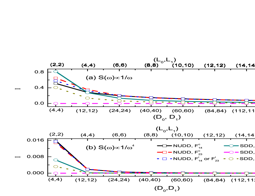
Figure 1: The factor $I$ as a function of the number of pulses $(L_{0},L_{1})$ for NUDD sequence (squares) and $(D_{0},D_{1})$ for SDD sequence (circles). The pulse sequences are compared for different filter functions $F(z)$ under the spectra (a) $S(\omega)\propto 1/\omega$ and (b) $S(\omega)\propto 1/\omega^{4}$, see Eq.(25).

Now, the performances of NUDD and SDD sequences in the two limiting cases, a common bath and two separated baths, are discussed. To ensure a relative fair comparison, in this study we assume both the total number of pulses and the total pulse sequence durations are the same for these two schemes, i.e. $L_{0}+(L_{0}+1)L_{1}=D_{0}+D_{1}$ and $T^{NUDD}=T^{SDD}$. In figure 1, the factor $I$[28], see Eq.(25), is used to measure the performances of NUDD and SDD sequences for different filter functions $F_{14}^{c}$, $F_{23}^{c}$, $F_{14}^{i}$ and $F_{23}^{i}$ under the spectra $S(\omega)\propto 1/\omega$ and $S(\omega)\propto 1/\omega^{4}$. The factors for different filter functions with the same sequence have obviously different performances if the number of pulses is small, while they almost coincide if the number of pulses becomes larger. In addition, the evaluation of the factor shows that SDD performs better than NUDD for the same filter function under $S(\omega)\propto 1/\omega$, while under $S(\omega)\propto 1/\omega^{4}$ NUDD performs similarly to SDD but is still outperformed by SDD over the range of larger number of pulses. Note that there is a special dot $(D_{0},D_{1})=(4,4)$ for the SDD sequence with filter function $F_{14}^{c}$, where it performs abnormally and worse than NUDD for the same filter function. We will come back to this point below. It is also interesting to notice that the data for SDD with $F_{23}^{c}$ is always zero but it is not for NUDD sequence with $F_{23}^{c}$. This means if the qubits are coupled to a common reservoir, SDD helps to protect the decoherence-free subspace while NUDD destroys it.

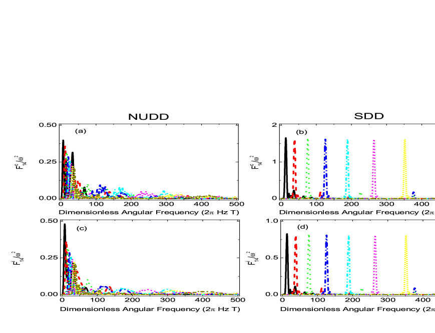
Figure 2: Modified filter functions, $F_{14}^{c}/\omega^{2}$ and $F_{14}^{i}/\omega^{2}$, as a function of dimensionless angular frequency $(\omega T)$  for NUDD and SDD sequences with the total pulse numbers studied in figure 1. This figure is related to the coherencce time regime and its layout is referred to reference[22].

Then, we employ the newly proposed approach[22],including the figure layout, to discuss why SDD performs better than NUDD and this question can be clarified in the coherence time regime. The coherence time regime is a range of frequency for a filter function, in which the error probabilities of several tens of percent are accepted. The accumulated error leading to decoherence in this regime is very large. For clarity, we focus on the filter functions, $F_{14}^{c}$ and $F_{14}^{i}$, and wrap the $1/\omega^{2}$ term into these functions, yielding modified filter functions $F_{14}^{c}/\omega^{2}$ and $F_{14}^{i}/\omega^{2}$. As shown in Eq.(23), the decoherence function $\chi(T)$ consists of the product of the spectrum $S(\omega)$ and the modified filter function. The decoherence function is minimum if the overlap between $S(\omega)$ and the modified filter function is minimum. The power law spectrum $S(\omega)$ considered here is a strong low-frequency noise and the intensity decreases as frequency increases. Smaller values of modified filter functions in the low-frequency spectral regime will lead to smaller values of decoherence function $\chi(T)$, and hence smaller factor $I$, supposing $T^{NUDD}=T^{SDD}$. In figure 2, the filter functions as a function of dimensionless angular frequency is shown for NUDD and SDD sequences with the pulse numbers considered in figure 1. As expected, both NUDD and SDD serve as high-pass filters and increasing total pulse number corresponds to a shift in spectral peak towards higher frequencies. Thus figure 1 reveals that the factor $I$ decreases with pulse number increasing. Furthermore, comparing figure 2(a) with figure 2(b) and figure 2(c) with figure 2(d), we observe the modified filter function for SDD peaks at higher frequencies than that for NUDD with the same total pulse number when this number becomes larger. Therefore, SDD performs better than NUDD when the pulse number is large, as shown in figure 1. However, compared with SDD, the modified filter function $F_{14}^{c}/\omega^{2}$ for NUDD peaks at almost the same frequencies but has a smaller value when the pulse number is small, such as $(L_{0},L_{1})=(2,2)$ or $(D_{0},D_{1})=(4,4)$. So it can be expected that NUDD performs better than SDD for filter function $F_{14}^{c}$ with this small pulse number, as shown in figure 1.

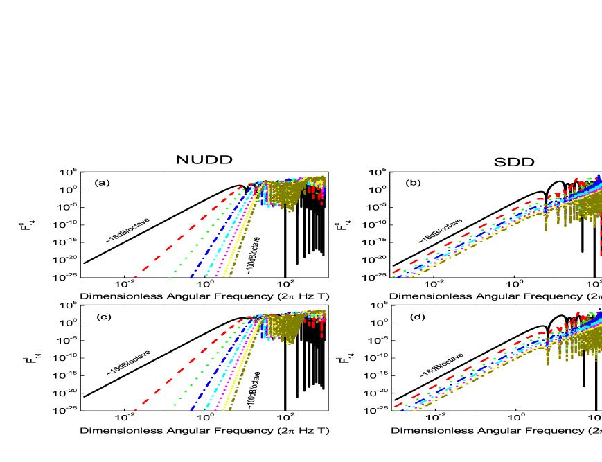
Figure 3: Log-Log plot of the filter functions, $F_{14}^{c}$ and $F_{14}^{i}$, as a function of dimensionless angular frequency $(\omega T)$  for NUDD and SDD sequences with the total pulse numbers studied in figure 1. This figure is related to the high-fidelity regime and its layout is referred to reference[22].

Here, the comparison of the filter functions between NUDD and SDD in another regime of interest, the high-fidelity regime, is also given. The high-fidelity regime, like the coherence time regime, is a range of frequency for a filter function, but in this regime the accumulated error bringing about decoherence is small. It turns up at short times $t\ll T_{2}$, where $T_{2}$ is the $1/e$ coherence time of a system. As before, we restrict our attention to the filter functions $F_{14}^{c}$ and $F_{14}^{i}$. The filter functions for the high-fidelity regime are shown graphically in figure 3, where the filter functions of NUDD and SDD are presented on a log-log plot for various values of $(L_{0},L_{1})$ or $(D_{0},D_{1})$. From figure 3(a) and 3(c), we find that NUDD sequence provides a filter function whose low-frequency rolloff increases from $\backsim 18$dB/octave to $\backsim 100$dB/octave as pulse number increases from $(L_{0},L_{1})=(2,2)$ to $(L_{0},L_{1})=(16,16)$. By contrast, the low-frequency rolloff for SDD is approximately constant, $\backsim 18$dB/octave, with each $(D_{0},D_{1})$. Here, rolloff is a term describing the steepness between the passband and the stopband of a filter function. The filter filters the noise in the stopband more efficiently, when the rolloff is steeper. Increasing rolloff means increasing the order of a filter and bringing the filter closer to the ideal response. If the rolloff is $6\eta dB/octave$, the order of the filter is considered as $\eta$. Then, as the total pulse number increases gradually, the filter order for NUDD becomes higher while the filter order for SDD stays about the same. Therefore, NUDD gives more flexibility and performs better than SDD, in terms of suppressing the low-frequency noise. Note that the performances of NUDD and SDD are analogous to the performances of UDD and CPMG in the high-fidelity regime for a single qubit, respectively[22]. The coherence time regime is concerned with the decoherence function while the high-fidelity regime provides small contributions to decoherence, but the high-fidelity regime draws more stringent scrutiny than the coherence time regime, because the high-fidelity regime is connected with predicted fault-tolerance error thresholds of $p_{th}=0.01\%$ derived from quantum error correction and the maximum allowable error must not surpass $p_{th}$ in quantum computing applications[22]. The illustration about these two regimes here helps to understand what changes when the pulses have nonzero $\tau_{\pi}$ in the following.

Now let us compare the finite-width filter function with the ideal filter function[25, 22] to find out what is affected by the finite-width pulses. In figure 4, we plot the ratio of the finite-width filter function $F_{14}^{c,r}$ (or $F_{14}^{i,r}$) to the ideal filter function $F_{14}^{c}$(or $F_{14}^{i}$) for NUDD and SDD with a given total pulse number and here we set $(L_{0},L_{1})=(6,6)$ or $(D_{0},D_{1})=(24,24)$. In these figures different traces correspond to different values of $\tau_{\pi}$ in units of the total pulse duration time $T$. From figure 4(a) and 4(c), it can be seen that the filter function for NUDD is affected in both coherence time regime and high-fidelity regime, still there is a mid frequency range which is nearly unaffected. Moreover, as the pulse duration $\tau_{\pi}$ increases, the influence on the filter function in the high-fidelity regime is more remarkable, and the mid frequency range becomes narrower. In comparison, figure 4(b) and 4(c) show that the filter function for SDD is nearly unaffected in the high-fidelity regime while the magnitude of the changes in coherence time regime is larger than that for NUDD. Similarly, for SDD the range which is nearly unaffected becomes narrower with the increasing of pulse duration $\tau_{\pi}$.

Fig.4 is ploted numerically, in which the sampling step is $0.0001$ from $0.001$ to $10$ and $100$ from $10$ to $10^{8}$. In the following, more details will be present. We first give out the analytical expression about the ratio of the finite-width filter function to the ideal fiter function. For convenience, we focus on the case of two independent reservoirs and the expression for SDD reads

$$R_{SDD} =\frac{F_{14,SDD}^{i,r}}{F_{14,SDD}^{i}}$$ (53)

$$=\cos^{2}(\frac{\omega\tau_{\pi}}{2})+\frac{\sin^{2}(\frac{\omega\tau_{\pi}}{4})}{\sin^{2}(\frac{\omega T}{4D_{j}})}\cos(\frac{\omega T}{2D_{j}})[\frac{\sin^{2}(\frac{\omega\tau_{\pi}}{4})}{\sin^{2}(\frac{\omega T}{4D_{j}})}\cos(\frac{\omega T}{2D_{j}})+2\cos(\frac{\omega\tau_{\pi}}{2})\cos(\omega T)]$$

It can be seen from Eq.(53) that there are singular points $\omega T=4kD_{j}\pi$, with $k$ being integral number and $\sin^{2}(\frac{\omega\tau_{\pi}}{4})\neq 0$. On the other hand, the expression for NUDD is written as

$$R_{NUDD} =\frac{F_{14,NUDD}^{i,r}}{F_{14,NUDD}^{i}}$$ (54)

$$=\frac{(f_{Re}^{(0),r})^{2}+(f_{Im}^{(0),r})^{2}+(f_{Re}^{(1),r})^{2}+(f_{Im}^{(1),r})^{2}}{(f_{Re}^{(0)})^{2}+(f_{Im}^{(0)})^{2}+(f_{Re}^{(1)})^{2}+(f_{Im}^{(1)})^{2}}$$

where $f_{Re}^{(n)}$, $f_{Im}^{(n)}$ and $f_{Re}^{(n),r}$, $f_{Im}^{(n),r}$ $(n=0,1)$ are real parts and image parts of the ideal filter function and of the imperfect filter function, respectively. They are given by

$$f_{NUDD}^{(n)}=f_{Re}^{(n)}+if_{Im}^{(n)}$$ (55)

$$f_{NUDD}^{(n),r}=f_{Re}^{(n),r}+if_{Im}^{(n),r}$$ (56)

with

$$f_{Re}^{(1)}=\sum\limits_{l_{1}=-L_{1}-1}^{L_{1}}(-1)^{l_{1}}\{\cos(\frac{\omega T}{2})\cos[\frac{\omega T}{2}\cos(\frac{l_{1}\pi}{L_{1}+1})]+\sin(\frac{\omega T}{2})\sin[\frac{\omega T}{2}\cos(\frac{l_{1}\pi}{L_{1}+1})]\}$$ (57)

$$f_{Im}^{(1)}=\sum\limits_{l_{1}=-L_{1}-1}^{L_{1}}(-1)^{l_{1}}\{-\cos(\frac{\omega T}{2})\sin[\frac{\omega T}{2}\cos(\frac{l_{1}\pi}{L_{1}+1})]+\sin(\frac{\omega T}{2})\cos[\frac{\omega T}{2}\cos(\frac{l_{1}\pi}{L_{1}+1})]\}$$ (58)

$$f_{Re}^{(0)}=\sum\limits_{l_{1}=0}^{L_{1}}\sum\limits_{l_{0}=-L_{0}-1}^{L_{0}}(-1)^{l_{0}}\{\cos(\frac{\omega\tau_{l_{1}}}{2})\cos[\frac{\omega\tau_{l_{1}}}{2}\cos(\frac{l_{0}\pi}{L_{0}+1})]+\sin(\frac{\omega\tau_{l_{1}}}{2})\sin[\frac{\omega\tau_{l_{1}}}{2}\cos(\frac{l_{0}\pi}{L_{0}+1})]\}$$ (59)

$$f_{Im}^{(0)}=\sum\limits_{l_{1}=0}^{L_{1}}\sum\limits_{l_{0}=-L_{0}-1}^{L_{0}}(-1)^{l_{0}}\{-\cos(\frac{\omega\tau_{l_{1}}}{2})\sin[\frac{\omega\tau_{l_{1}}}{2}\cos(\frac{l_{0}\pi}{L_{0}+1})]+\sin(\frac{\omega\tau_{l_{1}}}{2})\cos[\frac{\omega\tau_{l_{1}}}{2}\cos(\frac{l_{0}\pi}{L_{0}+1})]\}$$ (60)

$$f_{Re}^{(1),r}=\cos(\frac{\omega\tau_{\pi}}{2})f_{Re}^{(1)}+4\sin^{2}(\frac{\omega\tau_{\pi}}{4})\sin^{2}(\frac{\omega T}{2})$$ (61)

$$f_{Im}^{(1),r}=\cos(\frac{\omega\tau_{\pi}}{2})f_{Im}^{(1)}+2\sin^{2}(\frac{\omega\tau_{\pi}}{4})\sin(\omega T)$$ (62)

$$f_{Re}^{(0),r}=\cos(\frac{\omega\tau_{\pi}}{2})f_{Re}^{(0)}+4\sin^{2}(\frac{\omega\tau_{\pi}}{4})\sum\limits_{l_{1}=0}^{L_{1}}\sin^{2}(\frac{\omega\tau_{l_{1}}}{2})$$ (63)

$$f_{Im}^{(0),r}=\cos(\frac{\omega\tau_{\pi}}{2})f_{Im}^{(0)}+2\sin^{2}(\frac{\omega\tau_{\pi}}{4})\sum\limits_{l_{1}=0}^{L_{1}}\sin(\omega\tau_{l_{1}})$$ (64)

It is a tough task to list the singular points of Eq.(54) one by one, but we can study this problem numerically. Figure 5 is the enlarged view of figure 4(c) and (d) within three ranges, i.e. from $250$ to $1000$, from $9.99\times 10^{5}$ to $1\times 10^{6}$ and from $3.999\times 10^{6}$ to $4\times 10^{6}$. From figure 5(a), we can see that the singular points appear periodically for the SDD sequency, as predicted by Eq.(53). However, figure 5(b) indicates that no periodical singular points are obtained within the ranges considered. Therefore, the filter function for SDD is nearly unaffected in the high-fidelity regime, that is, before the first singular point $(\omega T=4D_{j}\pi=96\pi\approx 300,D_{j}=24)$ appears. In addition, SDD is affected by imperfect control pulses in the coherence time regime, that is, after the first singular point $(\omega T\approx 300)$ presents. The numerical results also suggest that in the coherence time regime the realistic filter function of NUDD is nearly equivalent to the ideal filter function.

4 Conclusions

In this paper we aim to provide some guidelines in the choice of sequences to be applied in experiments on the suppression of decoherence for a multi-qubit system. We derived the filter functions for NUDD and SDD sequences with zero-width or finite-width pulses in the pure-dephasing spin-boson model. The filter design perspective was used to analyze the performances of these sequences. The performances of two qubits initially in X state were discussed in detail.

The analysis shows that SDD outperforms NUDD for the bath with a soft cutoff while NUDD approaches SDD as the cutoff becomes harder. Second, if the qubits are coupled to a common reservoir, SDD helps to protect the decoherence-free subspace while NUDD destroys it. Third, when the imperfect control pulses with finite width are considered, NUDD is affected in both the high-fidelity regime and coherence time regime while SDD is obviously affected in the coherence time regime only. Note that SDD scheme protects multiqubit systems using multi-qubit operations while NUDD do it using only single-qubit operations. Therefore, future work for SDD will analyze the effect of the precision, with which pulse location of each qubit in a multi-qubit operation is specified. In addition, the discussion for the case with more than two qubits will be given.

References

List of figures

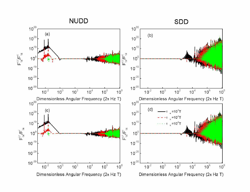
Figure 4: The ratio of the finite-width filter function $F_{14}^{c,r}$ (or $F_{14}^{i,r}$) to the ideal filter function $F_{14}^{c}$(or $F_{14}^{i}$) for NUDD with $(L_{0},L_{1})=(6,6)$ and SDD with $(D_{0},D_{1})=(24,24)$. In these figures different traces correspond to different values of $\tau_{\pi}$ in units of the total pulse duration time $T$.

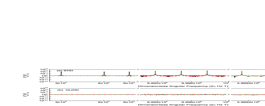
Figure 5: Enlarged view of figure 4(c) and (d) within the dimensionless angular frequency ranges from $250$ to $1000$, from $9.99\times 10^{5}$ to $1\times 10^{6}$ and from $3.999\times 10^{6}$ to $4\times 10^{6}$ for (a) SDD sequence and (b) NUDD sequence. The parameters are the same as that of figure 4.

References

- [1] M. Paternostro, M. S. Tame, G. M. Palma, and M. S. Kim. Entanglement generation and protection by detuning modulation. Phys. Rev. A, 74:052317, Nov 2006.
- [2] Rosario Franco, Giuseppe Compagno, Antonino Messina, and Anna Napoli. Generation of entangled two-photon binomial states in two spatially separate cavities. Open Systems & Information Dynamics, 13:463–470, 2006.
- [3] Jing Zhang, Yu-xi Liu, Chun-Wen Li, Tzyh-Jong Tarn, and Franco Nori. Generating stationary entangled states in superconducting qubits. Phys. Rev. A, 79:052308, May 2009.
- [4] Bruno Bellomo, Rosario Lo Franco, Sabrina Maniscalco, and Giuseppe Compagno. Entanglement trapping in structured environments. Phys. Rev. A, 78:060302, Dec 2008.
- [5] Bruno Bellomo, Rosario Lo Franco, and Giuseppe Compagno. Long-time preservation of nonlocal entanglement. Advanced Science Letters, 2(4):459–462, 2009.
- [6] Lorenza Viola and Seth Lloyd. Dynamical suppression of decoherence in two-state quantum systems. Phys. Rev. A, 58:2733–2744, Oct 1998.
- [7] Lorenza Viola, Emanuel Knill, and Seth Lloyd. Dynamical decoupling of open quantum systems. Phys. Rev. Lett., 82:2417–2421, Mar 1999.
- [8] E. L. Hahn. Spin echoes. Phys. Rev., 80:580–594, Nov 1950.
- [9] W.-K. Rhim, A. Pines, and J. S. Waugh. Violation of the spin-temperature hypothesis. Phys. Rev. Lett., 25:218–220, Jul 1970.
- [10] M. Mehring. Principles of high-resolution NMR in solids. Springer-Verlag in Berlin, New York, 1983.
- [11] U. Haeberlen. High Resolution NMR in Solids: Selective Averaging. Academic Press, New York, 1976.
- [12] H. Y. Carr and E. M. Purcell. Effects of diffusion on free precession in nuclear magnetic resonance experiments. Phys. Rev., 94:630–638, May 1954.
- [13] S. Meiboom and D. Gill. Modified spin-echo method for measuring nuclear relaxation times. Review of Scientific Instruments, 29(8):688 –691, Aug 1958.
- [14] K. Khodjasteh and D. A. Lidar. Fault-tolerant quantum dynamical decoupling. Phys. Rev. Lett., 95:180501, Oct 2005.
- [15] Kaveh Khodjasteh and Daniel A. Lidar. Performance of deterministic dynamical decoupling schemes: Concatenated and periodic pulse sequences. Phys. Rev. A, 75:062310, Jun 2007.
- [16] Xinhua Peng, Dieter Suter, and Daniel A Lidar. High fidelity quantum memory via dynamical decoupling: theory and experiment. Journal of Physics B: Atomic, Molecular and Optical Physics, 44(15):154003, 2011.
- [17] Götz S. Uhrig. Keeping a quantum bit alive by optimized -pulse sequences. Phys. Rev. Lett., 98:100504, Mar 2007.
- [18] Goren Gordon and Gershon Kurizki. Universal dephasing control during quantum computation. Phys. Rev. A, 76:042310, Oct 2007.
- [19] Musawwadah Mukhtar, Thuan Beng Saw, Wee Tee Soh, and Jiangbin Gong. Universal dynamical decoupling: Two-qubit states and beyond. Phys. Rev. A, 81:012331, Jan 2010.
- [20] Musawwadah Mukhtar, Wee Tee Soh, Thuan Beng Saw, and Jiangbin Gong. Protecting unknown two-qubit entangled states by nesting uhrig’s dynamical decoupling sequences. Phys. Rev. A, 82:052338, Nov 2010.
- [21] Zhen-Yu Wang and Ren-Bao Liu. Protection of quantum systems by nested dynamical decoupling. Phys. Rev. A, 83:022306, Feb 2011.
- [22] M. J. Biercuk, A. C. Doherty, and H. Uys. Dynamical decoupling sequence construction as a filter-design problem. Journal of Physics B: Atomic, Molecular and Optical Physics, 44(15):154002, 2011.
- [23] Götz S. Uhrig. Exact results on dynamical decoupling by pulses in quantum information processes. New Journal of Physics, 10(8):083024, 2008.
- [24] B. Lee, W. M. Witzel, and S. Das Sarma. Universal pulse sequence to minimize spin dephasing in the central spin decoherence problem. Phys. Rev. Lett., 100:160505, Apr 2008.
- [25] Michael J. Biercuk, Hermann Uys, Aaron P. VanDevender, Nobuyasu Shiga, Wayne M. Itano, and John J. Bollinger. Optimized dynamical decoupling in a model quantum memory. Nature, 458:996, 2009.
- [26] Michael J. Biercuk, Hermann Uys, Aaron P. VanDevender, Nobuyasu Shiga, Wayne M. Itano, and John J. Bollinger. Experimental uhrig dynamical decoupling using trapped ions. Phys. Rev. A, 79:062324, Jun 2009.
- [27] Hermann Uys, Michael J. Biercuk, and John J. Bollinger. Optimized noise filtration through dynamical decoupling. Phys. Rev. Lett., 103:040501, Jul 2009.
- [28] S. Pasini and G. S. Uhrig. Optimized dynamical decoupling for power-law noise spectra. Phys. Rev. A, 81:012309, Jan 2010.
- [29] K. Hornberger. Introduction to decoherence theory. In Andreas Buchleitner, Carlos Viviescas, and Markus Tiersch, editors, Entanglement and Decoherence, volume 768 of Lecture Notes in Physics, pages 221–276. Springer Berlin Heidelberg, 2009.
- [30] Kaveh Khodjasteh and Lorenza Viola. Dynamical quantum error correction of unitary operations with bounded controls. Phys. Rev. A, 80:032314, Sep 2009.
- [31] G. S. Agarwal. Saving entanglement via a nonuniform sequence of pulses. Physica Scripta, 82(3):038103, 2010.
- [32] E. C. G. Sudarshan. Equivalence of semiclassical and quantum mechanical descriptions of statistical light beams. Phys. Rev. Lett., 10:277–279, Apr 1963.
- [33] Roy J. Glauber. Photon correlations. Phys. Rev. Lett., 10:84–86, Feb 1963.
- [34] Götz S Uhrig. Exact results on dynamical decoupling by pulses in quantum information processes. New Journal of Physics, 10(8):083024, 2008.
- [35] Łukasz Cywiński, Roman M. Lutchyn, Cody P. Nave, and S. Das Sarma. How to enhance dephasing time in superconducting qubits. Phys. Rev. B, 77:174509, May 2008.
- [36] Kaveh Khodjasteh and Daniel A. Lidar. Rigorous bounds on the performance of a hybrid dynamical-decoupling quantum-computing scheme. Phys. Rev. A, 78:012355, Jul 2008.