Sparse Pseudospectral Approximation Method

Abstract

Multivariate global polynomial approximations – such as polynomial chaos or stochastic collocation methods – are now in widespread use for sensitivity analysis and uncertainty quantification. The pseudospectral variety of these methods uses a numerical integration rule to approximate the Fourier-type coefficients of a truncated expansion in orthogonal polynomials. For problems in more than two or three dimensions, a sparse grid numerical integration rule offers accuracy with a smaller node set compared to tensor product approximation. However, when using a sparse rule to approximately integrate these coefficients, one often finds unacceptable errors in the coefficients associated with higher degree polynomials.

By reexamining Smolyak’s algorithm and exploiting the connections between interpolation and projection in tensor product spaces, we construct a sparse pseudospectral approximation method that accurately reproduces the coefficients for basis functions that naturally correspond to the sparse grid integration rule. The compelling numerical results show that this is the proper way to use sparse grid integration rules for pseudospectral approximation.

1 Introduction

As the power and availability of computers has increased, the profile of simulation in scientific and engineering endeavors has risen. Computer simulations that model complex physical phenomena now regularly aid in decision making and design processes. However, the complexity and computational cost of the codes often render them impractical for design and uncertainty studies, where many runs at different input parameter values are necessary to compute statistics of interest. In such cases, designers use a relatively small number of high fidelity runs to build cheaper surrogate models, which are then used for the studies requiring many model evaluations.

It is now common to use a multivariate global polynomial of the input parameters as the surrogate, particularly when one desires estimates of integrated quantities such as mean and variance of simulation results. Additionally, the polynomial surrogate is typically much cheaper to evaluate as a function of the input parameters, which allows sampling and optimization studies at a fraction of the cost. In an uncertainty quantification context – where the input parameters often carry the interpretation of random variables – this polynomial approximation method appears under the labels polynomial chaos [1, 2] or stochastic collocation [3, 4], amongst others.

One of the primary disadvantages of the polynomial methods is the rapid growth in the work required to compute the approximation as the number of model input parameters increases; this generally limits the applicability of these methods to models with fewer than ten input parameters. To combat this apparent curse of dimensionality, many have proposed to use so-called sparse grid methods [5], which deliver comparable accuracy for some problems using far fewer function evaluations to build the surrogate. The sparse grid is a set of points in the input parameter space that is the union of carefully chosen tensor product grids. When the tensor grids are formed from univariate point sets with a nesting property, such as the Chebyshev points, the number of points in the union of tensor grids is greatly reduced – although this nesting feature is not necessary for the construction of the sparse grids. The points in the sparse grid can be used as a numerical integration rule [6, 7], where the weights are linear combinations of weights from the member tensor grids. Alternatively, the interpolating tensor product Lagrange polynomials constructed on the member tensor grids can be linearly combined in a similar fashion to yield a polynomial surrogate [8], since a linear combination of polynomials is itself a polynomial.

Another popular polynomial representation employs a multivariate orthogonal polynomial basis. When the coefficients of a series in this basis are computed by projecting the unknown function onto each basis, the series is a spectral projection or Fourier series [9, 10]; this is also known as the polynomial chaos expansion in an uncertainty quantification context [1, 2]. The series must be truncated for computation; convergence to the true function occurs in the mean-squared sense as one adds more basis polynomials. If the integrals in the projections are approximated with a numerical integration rule, this method is known as a pseudospectral projection [11, 12]. These integral approximations only require the simulation outputs evaluated at the quadrature points of the input space.

The question that naturally arises is: Which numerical integration rule is appropriate to approximate the Fourier coefficients? Some early attempts used Monte Carlo integration [13], but its relative inaccuracies overwhelm the spectral accuracy of the truncated Fourier series. Other attempts used tensor product Gaussian quadrature rules, but they do not scale to high dimensional parameter spaces due to the exponential increase in the number of quadrature points with dimension. The sparse-grid quadrature rules have shown promise for retaining the spectral accuracy while alleviating the curse of dimensionality. However, in practice this approach produces unacceptable errors in the coefficients associated with the higher order basis polynomials, which forces a much stricter truncation than might be expected for the number of function evaluations [14].

This paper presents a sparse pseudospectral approximation method (SPAM) for computing the coefficients of the truncated Fourier series with the points of the sparse grid integration rule that eliminates the error in the coefficients associated with higher degree polynomials. This allows the number of terms in the expansion to be consistent with the number of points in the sparse-grid integration rule. The key is to separately compute the coefficients of a tensor product polynomial expansion for each tensor grid in the sparse grid. The linear combination of the tensor weights used to produce the sparse-grid integration weights is then used to linearly combine the coefficients of each tensor expansion. We show that this method produces a pointwise equivalent polynomial surrogate to the one constructed from a linear combination of tensor product Lagrange polynomials. Therefore error bounds from that context can be applied directly.

Recently, in the context of spectral methods for discretized PDEs, Shen and coauthors [15, 16] proposed and analyzed a closely related sparse spectral approximation using a hierarchical basis of Chebyshev polynomials; the hierarchical structure results in increased efficiency. Their computation of the coefficients for the hierarchical basis follow a comparable construction to the one we present. However, their focus is on approximating the solution to a high-dimensional PDE, as opposed to more general function approximation.

The remainder of the paper is structured as follows. In Section 2, we review the relationship between Lagrange polynomial interpolation on a set of quadrature points and the pseudospectral approximation for univariate functions; we then extend this analysis to multivariate tensor product approximation. Section 2 closes with a review of Smolyak’s algorithm. In Section 3, we detail the SPAM for approximating the Fourier coefficients using the function evaluations at the sparse-grid integration points followed by some interesting analysis results. In Section 4, we present numerical experiments from (i) a collection of scalar bivariate functions and (ii) an elliptic PDE model with parameterized coefficients. In each experiment, we compare the approximate Fourier coefficients from the SPAM with ones computed directly with the sparse grid integration rule. Finally we conclude with a summary and discussion in Section 5.

2 Background and Problem Set-up

In this section, we briefly review the background necessary to understand the SPAM; in particular, we examine the relationship between the Lagrange interpolation on a set of Gaussian quadrature points and a pseudospectral approximation in a basis of orthonormal polynomials. One purpose of this review is to set up the notation, which departs slightly from the notation in the disparate references. For the orthogonal polynomials, we follow the notation of [17].

Consider a multivariate function $f:\mathcal{S}\rightarrow\mathbb{R}$, where the domain $\mathcal{S}\subset\mathbb{R}^{d}$ has a product structure

$$\mathcal{S}=\mathcal{S}_{1}\times\cdots\times\mathcal{S}_{d}.$$ (1)

Define a $d$-dimensional point $s=(s_{1},\dots,s_{d})\in\mathcal{S}$. The domain is equipped with a positive, separable weight function $w:\mathcal{S}\rightarrow\mathbb{R}_{+}$ where $w(s)=w_{1}(s_{1})\cdots w_{d}(s_{d})$ and

$$\int_{\mathcal{S}_{k}}s_{k}^{a}\,w_{k}(s_{k})\,ds_{k}<\infty,\qquad k=1,\dots,d,\quad a=1,2,\dots$$ (2)

The $w_{k}$ are normalized to integrate to 1, which allows the interpretation of $w(s)$ as a probability density function. In general, we consider functions which are square-integrable on $\mathcal{S}$, i.e.

$$\int_{\mathcal{S}}f(s)^{2}\,w(s)\,ds\;<\;\infty.$$ (3)

Such functions admit a convergent Fourier series in orthonormal basis polynomials,

$$f(s)\;=\;\sum_{i_{1}=1}^{\infty}\cdots\sum_{i_{d}=1}^{\infty}\hat{f}_{i_{1},\dots,i_{d}}\,\pi_{i_{1}}(s_{1})\cdots\pi_{i_{d}}(s_{d})\;=\;\sum_{\mathbf{i}\in\mathbb{N}^{d}}\hat{f}_{\mathbf{i}}\,\pi_{\mathbf{i}}(s),$$ (4)

where the equality is in the $L_{2}$ sense, $\mathbf{i}=(i_{1},\dots,i_{d})$ is a multi-index, and

$$\hat{f}_{\mathbf{i}}\;=\;\int_{\mathcal{S}}f(s)\,\pi_{\mathbf{i}}(s)\,w(s)\,ds$$ (5)

is the Fourier coefficient associated with the basis polynomial $\pi_{\mathbf{i}}(s)$. The $\pi_{i_{k}}(s_{k})$ are univariate polynomials in $s_{k}$ of degree $i_{k}-1$ that are orthonormal with respect to $w_{k}(s_{k})$. In general, a pseudospectral method uses a numerical integration rule to approximate a subset of the integrals (5); the remaining terms are discarded.

While any square-integrable function admits a convergent Fourier series in theory, the polynomial approximation methods perform best on a much smaller class of smooth functions; we will restrict our attention to such function classes when citing appropriate error bounds. Before diving into the multivariate approximation, we first review the univariate case.

2.1 Gaussian Quadrature, Collocation, Pseudospectral Methods

Consider the problem set-up above with $d=1$. Let $\mbox{\boldmath$\pi$}(s)=[\pi_{1}(s),\dots,\pi_{n}(s)]^{T}$ be a vector of the first $n$ polynomials that are orthonormal with respect to the weight function $w(s)$. The components of $\mbox{\boldmath$\pi$}(s)$ satisfy a recurrence relationship, which we can write in matrix form as

$$s\mbox{\boldmath$\pi$}(s)=\mathbf{J}\mbox{\boldmath$\pi$}(s)+\beta_{n+1}\pi_{n+1}(s)\mathbf{e}_{n},$$ (6)

where $\mathbf{e}_{n}$ is an $n$-vector of zeros with a one in the last entry, and $\mathbf{J}$ (known as the Jacobi matrix) is the symmetric, tridiagonal matrix containing the recurrence coefficients,

$$\mathbf{J}=\begin{bmatrix}\alpha_{1}&\beta_{1}&&&\\ \beta_{2}&\alpha_{2}&\beta_{3}&&\\ &\ddots&\ddots&\ddots&\\ &&\beta_{n-1}&\alpha_{n-1}&\beta_{n}\\ &&&\beta_{n}&\alpha_{n}\end{bmatrix}.$$ (7)

The zeros of $\pi_{n+1}(s)$ generate eigenvalue/eigenvector pairs of $\mathbf{J}$ by (6), which we write

$$\mathbf{J}=\mathbf{Q}\Lambda\mathbf{Q}^{T},\qquad\Lambda=\mathrm{diag}\big{(}[\lambda_{1},\dots,\lambda_{n}]\big{)},$$ (8)

where $\mathbf{Q}(i,j)=\pi_{i}(\lambda_{j})/\|\mbox{\boldmath$\pi$}(\lambda_{j})\|$ are the elements of the normalized eigenvectors. The zeros $\lambda_{j}$ of $\pi_{n+1}(s)$ are the points of the $n$-point Gaussian quadrature rule for $w(s)$; the quadrature weights $\nu_{j}\in\mathbb{R}_{+}$ are given by

$$\nu_{j}=\frac{1}{\|\mbox{\boldmath$\pi$}(\lambda_{j})\|^{2}},$$ (9)

which are the squares of the first component of the $j$th eigenvector. A Gaussian quadrature approximation to the integral is written

$$\int_{\mathcal{S}}f(s)\,w(s)\,ds\;\approx\;\mathcal{U}_{q}^{n}(f)\;=\;\sum_{j=1}^{n}f(\lambda_{j})\,\nu_{j}\;=\;\mathbf{f}^{T}\mbox{\boldmath$\nu$}.$$ (10)

The $\mathcal{U}_{q}^{n}$ denotes the linear operation of quadrature applied to $f$; the subscript $q$ is for quadrature. This notation will be used later when discussing sparse grids. The $n$-vector $\mathbf{f}$ contains the evaluations of $f(s)$ at the quadrature points, and the $n$-vector $\nu$ contains the weights of the quadrature rule. It will be notationally convenient to define the matrices

$$\mathbf{P}(i,j)=\pi_{i}(\lambda_{j}),\qquad\mathbf{W}=\mathrm{diag}([\sqrt{\nu_{1}},\dots,\sqrt{\nu_{n}}]),$$ (11)

and note that the orthogonal matrix of eigenvectors $\mathbf{Q}$ can be written $\mathbf{Q}=\mathbf{P}\mathbf{W}$.

The spectral collocation approximation of $f(s)$ constructs a Lagrange interpolating polynomial through the Gaussian quadrature points. Since the points are distinct, the $n-1$ degree interpolating polynomial is unique. We write this approximation $\mathcal{U}_{l}^{n}(f)$, where the subscript $l$ is for Lagrange interpolation, as

$$f(s)\;\approx\;\mathcal{U}_{l}^{n}(f)\;=\;\sum_{i=1}^{n}f(\lambda_{i})\,\ell_{i}(s)\;=\;\mathbf{f}^{T}\mathbf{l}(s).$$ (12)

The parameterized vector $\mathbf{l}(s)$ contains the Lagrange cardinal functions

$$\ell_{i}(s)=\prod_{j=1,\;j\not=i}^{n}\frac{s-\lambda_{j}}{\lambda_{i}-\lambda_{j}}.$$ (13)

By construction, the collocation polynomial $\mathcal{U}_{l}^{n}(f)$ interpolates $f(s)$ at the Gaussian quadrature points.

The pseudospectral approximation of $f(s)$ is constructed by first truncating its Fourier series at $n$ terms and approximating each Fourier coefficient with a quadrature rule. If we use the $n$-point Gaussian quadrature, then we can write the approximation as

$$f(s)\;\approx\;\mathcal{U}_{p}^{n}(f)\;=\;\sum_{i=1}^{n}\hat{f}_{i}\,\pi_{i}(s)\;=\;\hat{\mathbf{f}}^{T}\mbox{\boldmath$\pi$}(s),$$ (14)

where $\hat{f}_{i}$ is the pseudospectral coefficient,

$$\hat{f}_{i}=\sum_{j=1}^{n}f(\lambda_{j})\,\pi_{i}(\lambda_{j})\,\nu_{j},$$ (15)

and the vector $\hat{\mathbf{f}}$ contains all coefficient approximations; the subscript $p$ on $\mathcal{U}_{p}^{n}$ is for pseudospectral. Note that we have overloaded the notation by defining $\hat{f}_{i}$ as the pseudospectral coefficient (15), instead of the true Fourier coefficient in (5). We next state two lemmas about the relationship between the spectral collocation and pseudospectral approximations for future reference.

Lemma 1.

The vector of evaluations of $f$ at the quadrature points $\mathbf{f}$ is related to the pseudospectral coefficients $\hat{\mathbf{f}}$ by

$$\hat{\mathbf{f}}\;=\;\mathbf{Q}\mathbf{W}\mathbf{f}\;=\;\mathbf{P}\mathbf{W}^{2}\mathbf{f}.$$ (16)

Proof.

This is easily verified by equation (15) using the matrices defined in (11). ∎

Lemma 2.

The pseudospectral approximation $\mathcal{U}_{p}^{n}(f)$ is equal to the spectral collocation approximation $\mathcal{U}_{l}^{n}(f)$ for all $s\in\mathcal{S}$.

Proof.

By the uniqueness of the Lagrange polynomial interpolation, we can write $\mathbf{P}\mathbf{l}(s)=\mbox{\boldmath$\pi$}(s)$. Since $\mathbf{P}=\mathbf{Q}\mathbf{W}^{-1}$, we have $\mathbf{l}(s)=\mathbf{W}\mathbf{Q}^{T}\mbox{\boldmath$\pi$}(s)$. Then

$$\mathcal{U}_{l}^{n}(f) =\mathbf{f}^{T}\mathbf{l}(s)$$

$$=\mathbf{f}^{T}\mathbf{W}\mathbf{Q}^{T}\mbox{\boldmath$\pi$}(s)$$

$$=\hat{\mathbf{f}}^{T}\mbox{\boldmath$\pi$}(s)$$

$$=\mathcal{U}_{p}^{n}(f),$$

as required. ∎

Lemma 2 implies that the pseudospectral approximation $\mathcal{U}_{p}^{n}(f)$ interpolates $f(s)$ at the Gaussian quadrature points. However, the equivalence expressed in Lemma 2 breaks down in two important cases. When the number of terms in the orthogonal series is less than the number of points in the quadrature rules, the orthogonal series representation no longer produces the same polynomial as the Lagrange interpolant. Also, if a quadrature rule that is not the Gaussian quadrature rule is used to approximate the Fourier coefficients, then the discrete Fourier transform from Lemma 1 is no longer valid. The latter situation may occur if an alternative quadrature rule holds practical advantages over the Gaussian quadrature rule.

Remark 1.

We have restricted our attention to orthonormal polynomials and Gaussian quadrature rules for a given weight function. However, transformations similar to Lemma 1 apply for Chebyshev polynomials and Clenshaw-Curtis quadrature rules using a fast Fourier transform. For an insightful discussion of the comparisions between these methods of integration and approximation, see [18].

2.2 Tensor Product Extensions

When $d>1$, the above concepts extend directly via a tensor product construction. For a given multi-index $\mathbf{n}=(n_{1},\dots,n_{d})\in\mathbb{N}^{d}$, it is convenient to define the set of multi-indices

$$\mathcal{I}_{\mathbf{n}}=\{\mathbf{i}\;:\;\mathbf{i}\in\mathbb{N}^{d},\,1\leq i_{k}\leq n_{k},\,k=1,\dots,d\}.$$ (17)

We can use this index set to reference components of the tensor product approximations.

Tensor product Gaussian quadrature rules are constructed by taking cross products of univariate Gaussian quadrature rules. For multi-index $\mathbf{n}$, let $G_{\mathbf{n}}$ be the set of $d$-variate Gaussian quadrature points,

$$G_{\mathbf{n}}\;=\;\{\lambda_{\mathbf{i}}=(\lambda_{i_{1}},\dots,\lambda_{i_{d}})\;:\;\mathbf{i}\in\mathcal{I}_{\mathbf{n}}\},$$ (18)

where the points $\lambda_{i_{k}}$ with $i_{k}=1,\dots,n_{k}$ are the univariate quadrature points for $w_{k}(s_{k})$. The associated quadrature weights $W_{\mathbf{n}}$ are given by

$$W_{\mathbf{n}}\;=\;\big{\{}\,\nu_{\mathbf{i}}=\nu_{i_{1}}\cdots\nu_{i_{d}}\;:\;\mathbf{i}\in\mathcal{I}_{\mathbf{n}}\,\big{\}}.$$ (19)

In words, the tensor product quadrature weights are products of the univariate weights. To approximate the integral of $f(s)$, compute

$$\int_{\mathcal{S}}f(s)\,w(s)\,ds \approx(\mathcal{U}_{q}^{n_{1}}\otimes\cdots\otimes\mathcal{U}_{q}^{n_{d}})(f)$$

$$=\sum_{i_{1}=1}^{n_{1}}\cdots\sum_{i_{d}=1}^{n_{d}}f(\lambda_{i_{1}},\dots,\lambda_{i_{d}})\,\nu_{i_{1}}\cdots\nu_{i_{d}}$$

$$=\sum_{\mathbf{i}\in\mathcal{I}_{\mathbf{n}}}f(\lambda_{\mathbf{i}})\,\nu_{\mathbf{i}}$$

$$=\mathbf{f}_{\mathbf{n}}^{T}\,\mbox{\boldmath$\nu$}_{\mathbf{n}}$$

where $\mathbf{f}_{\mathbf{n}}$ is the vector of function evaluations at the tensor grid of quadrature points, and $\mbox{\boldmath$\nu$}_{\mathbf{n}}$ is a vector of the tensor product quadrature weights.

The spectral collocation approximation on the points $G_{\mathbf{n}}$ uses a basis of product-type Lagrange cardinal functions. Define the vector of these basis polynomials by

$$\mathbf{l}_{\mathbf{n}}(s)=\mathbf{l}_{n_{1}}(s_{1})\otimes\cdots\otimes\mathbf{l}_{n_{d}}(s_{d}),$$ (20)

where $\mathbf{l}_{n_{k}}(s_{k})$ is a vector of the univariate Lagrange cardinal functions constructed on the univariate quadrature rule defined by $\lambda_{i_{k}}$; see (13). Then the tensor product spectral collocation approximation for the multi-index $\mathbf{n}$ is given by

$$f(s) \approx(\mathcal{U}_{l}^{n_{1}}\otimes\cdots\otimes\mathcal{U}_{l}^{n_{d}})(f)$$ (21)

$$=\sum_{i_{1}=1}^{n_{1}}\cdots\sum_{i_{d}=1}^{n_{d}}f(\lambda_{i_{1}},\dots,\lambda_{i_{d}})\,\ell_{i_{1}}(s_{1})\cdots\ell_{i_{d}}(s_{d})$$ (22)

$$=\sum_{\mathbf{i}\in\mathcal{I}_{\mathbf{n}}}f(\lambda_{\mathbf{i}})\,\ell_{\mathbf{i}}(s)$$ (23)

$$=\mathbf{f}_{\mathbf{n}}^{T}\,\mathbf{l}_{\mathbf{n}}(s).$$ (24)

The tensor product pseudospectral approximation uses a product type multivariate orthonormal polynomial basis, which is simply a Kronecker product of the univariate orthonormal polynomials. For a multi-index $\mathbf{n}$, let $\mbox{\boldmath$\pi$}_{n_{k}}(s_{k})$ be the vector of univariate polynomials that are orthonormal with respect to $w_{k}(s_{k})$ for $k=1,\dots,d$. Then the vector

$$\mbox{\boldmath$\pi$}_{\mathbf{n}}(s)=\mbox{\boldmath$\pi$}_{n_{1}}(s_{1})\otimes\cdots\otimes\mbox{\boldmath$\pi$}_{n_{d}}(s_{d})$$ (25)

contains polynomials that are orthonormal with respect to $w(s)$; we can uniquely reference a component of the vector $\mbox{\boldmath$\pi$}_{\mathbf{n}}(s)$ by $\pi_{\mathbf{i}}(s)$ with $\mathbf{i}\in\mathcal{I}_{\mathbf{n}}$. The tensor product pseudospectral approximation for the multi-index $\mathbf{n}$ is given by

$$f(s) \approx\;(\mathcal{U}_{p}^{n_{1}}\otimes\cdots\otimes\mathcal{U}_{p}^{n_{d}})(f)$$ (26)

$$=\sum_{i_{1}=1}^{n_{1}}\cdots\sum_{i_{d}=1}^{n_{d}}\hat{f}_{i_{1},\dots,i_{d}}\,\pi_{i_{1}}(s_{1})\cdots\pi_{i_{d}}(s_{d})$$ (27)

$$=\sum_{\mathbf{i}\in\mathcal{I}_{\mathbf{n}}}\hat{f}_{\mathbf{i}}\,\pi_{\mathbf{i}}(s)$$ (28)

$$=\hat{\mathbf{f}}_{\mathbf{n}}^{T}\,\mbox{\boldmath$\pi$}_{\mathbf{n}}(s),$$ (29)

where $\hat{\mathbf{f}}_{\mathbf{n}}$ is the vector of pseudospectral coefficients

$$\hat{f}_{\mathbf{i}} =\sum_{j_{1}=1}^{n_{1}}\cdots\sum_{j_{d}=1}^{n_{d}}f(\lambda_{j_{1}},\dots,\lambda_{j_{d}})\,\pi_{i_{1}}(\lambda_{j_{1}})\cdots\pi_{i_{d}}(\lambda_{j_{d}})\,\nu_{j_{1}}\cdots\nu_{j_{d}}$$ (30)

$$=\sum_{\mathbf{j}\in\mathcal{I}_{\mathbf{n}}}f(\lambda_{\mathbf{j}})\,\pi_{\mathbf{i}}(\lambda_{\mathbf{j}})\,\nu_{\mathbf{j}}.$$ (31)

The extensions of Lemmas 1 and 2 are then straightforward. For the multi-index $\mathbf{n}$, define the matrices

$$\mathbf{Q}=\mathbf{Q}_{n_{1}}\otimes\cdots\otimes\mathbf{Q}_{n_{d}},\qquad\mathbf{P}=\mathbf{P}_{n_{1}}\otimes\cdots\otimes\mathbf{P}_{n_{d}},\qquad\mathbf{W}=\mathbf{W}_{n_{1}}\otimes\cdots\otimes\mathbf{W}_{n_{d}}.$$ (32)

The proofs of Lemmas 1 and 2 hold with

$$\mathbf{f}=\mathbf{f}_{\mathbf{n}},\qquad\hat{\mathbf{f}}=\hat{\mathbf{f}}_{\mathbf{n}},\qquad\mathbf{l}(s)=\mathbf{l}_{\mathbf{n}}(s),\qquad\mbox{\boldmath$\pi$}(s)=\mbox{\boldmath$\pi$}_{\mathbf{n}}(s).$$ (33)

This is easily verified by employing the mixed product property of Kronecker products. In words, we have that the Lagrange interpolant constructed on a tensor product of Gaussian quadrature points (i.e., tensor product collocation) produces the same polynomial approximation as a truncated Fourier expansion with a tensor product basis, where the coefficients are computed with the tensor product Gaussian quadrature rule (i.e., tensor product pseudospectral). This equivalence occurs when the number of quadrature points in each variable is equal to the number of univariate basis polynomials in each variable; in other words, the number of points is the maximum degree plus one in each variable.

2.3 Smolyak’s Algorithm and Sparse Grids

The inescapable challenge for tensor product approximation is the exponential increase in the work required to compute the approximation as the dimension increases. An $n$-point quadrature rule in each of $d$ dimensions uses $n^{d}$ function evaluations. Thus, tensor product approximation quickly becomes infeasible beyond a handful of dimensions. Smolyak’s algorithm [19] attempts to alleviate this curse of dimensionality while retaining integration and interpolation accuracy for certain classes of functions.

The majority of sparse grid applications in the literature rely on Smolyak’s algorithm. The most common derivation starts by defining a linear operation (e.g., integration, interpolation, or projection) on a univariate function. We can generalize the notation used in (10), (12), and (14) by writing the linear operation as $\mathcal{U}^{m}(f)$. However, it is common to reinterpret the parameter $m$ in this context as a choice for how the number of points grows as $m$ is incremented. For example, $n_{m}=m$ for $m>0$ would correspond to (10), (12), and (14). Another common growth relationship is

$$n_{m}=2^{m}-1,\quad m\geq 1.$$ (34)

Such a relationship is useful when the quadrature/interpolation point sets are nested, i.e., the points of the $n$-point rule are a subset of the points in the $2n+1$ rule. This notably occurs for rules based on (i) Chebyshev points [17], (ii) Gauss-Patterson quadrature formulas [20], or (iii) equidistant points. In the case of a closed region of interpolation/integration, one may include and reuse the endpoints of the interval in the sequence of approximations; see for example the popular Clenshaw-Curtis integration rules [21]. Nested point sets can greatly increase efficiency if $f(s)$ is very expensive.

Define $|\mathbf{m}|=m_{1}+\cdots+m_{d}$. Given a univariate linear operator, Smolyak’s method can be written

$$\mathcal{A}=\sum_{\mathbf{m}\in\mathcal{I}}c(\mathbf{m})\,(\mathcal{U}^{m_{1}}\otimes\cdots\otimes\mathcal{U}^{m_{d}}).$$ (35)

In the standard formulation [8, 6], the set of admissible multi-indices $\mathcal{I}$ is

$$\mathcal{I}\;=\;\big{\{}\,\mathbf{m}\in\mathbb{N}^{d}\;:\;l+1\leq|\mathbf{m}|\leq l+d\,\big{\}}$$ (36)

for a given level parameter $l$. In this case, the coefficients $c(\mathbf{m})$ are

$$c(\mathbf{m})\;=\;(-1)^{l+d-|\mathbf{m}|}\,{d-1\choose l+d-|\mathbf{m}|}.$$ (37)

However, adaptive and anisotropic versions of Smolyak’s algorithm may contain different choices for $\mathcal{I}$ and $c(\mathbf{m})$; such variations are useful if a function’s variability can be primarily attributed to a subset of the inputs. See [22, 23] for details on such methods.

For our purposes, it is sufficient to note that Smolyak’s algorithm amounts to a linear combination of tensor product operations. The specific tensor products are chosen so that no constituent tensor grid contains too many nodes. In the case of nested univariate rules, a node may be common to many tensor products. In practice, one may structure the computation to evaluate the function once per node in the union of tensor product grids – as opposed to once per node per tensor grid. This greatly simplifies the sparse grid integration, which can be written as a set of nodes and weights. If a node is common to multiple constituent tensor grids, then its corresponding weight is computed as a linear combination of the tensor grid weights; the coefficients of the linear combination are exactly $c(\mathbf{m})$. It is worth noting that the weights of a sparse grid rule can be negative, which precludes its use as a positive definite weighted inner product.

3 Sparse Pseudospectral Approximation Method

In practice, one may wish to take advantage of the relatively small number of points in the sparse grid quadrature rule when computing a pseudospectral approximation. This is often done by first truncating the Fourier series representation of $f(s)$ (see (5)), and then approximating its spectral coefficients with a sparse grid quadrature rule. Unfortunately, choosing the parameters of the sparse grid rule that will accurately approximate the integral formulation of the Fourier coefficient is not straightforward. The is because – in constrast to tensor product approximation – the Lagrange interpolating polynomial is not equivalent to a truncated pseudospectal approximation with sparse grid integration, where the number of basis polynomials is equal to the number of points in the quadrature rule. The general wisdom has been to truncate conservatively for a sparse grid quadrature rule constrained by a computational budget; such heuristics become more complicated when anisotropic sparse grid rules are used.

The SPAM approaches this problem from a different perspective; it is merely the proper application of Smolyak’s algorithm to the tensor product pseudospectral projection. We take advantage of the equivalence between tensor product pseudospectral and spectral collocation approximations to construct spectral approximations that naturally correspond to a given sparse grid quadrature rule. In essence, since the sparse grid quadrature rule is constructed by taking linear combinations of tensor product quadrature rules, we can take the same linear combination of tensor product pseudospectral expansions to produce an approximation in a basis of multivariate orthogonal polynomials; a linear combination of expansions can be easily computed by linearly combining the pseudospectral coefficients corresponding to the same basis polynomial. Each tensor product pseudospectral expansion is simply a transformation from the Lagrange basis using Lemma 1. In the numerical examples of Section 4, we show compelling evidence that this procedure is superior to directly applying the sparse grid quadrature rule to the integral formulation of the Fourier coefficients.

More precisely, let $\mathcal{I}$ and $c(\mathbf{m})$ be the admissible index set and coefficient function for a given sparse grid quadrature rule. Then the sparse pseudospectral approximation is given by

$$f(s) \approx\mathcal{A}_{p}(f)$$ (38)

$$=\sum_{\mathbf{m}\in\mathcal{I}}\,c(\mathbf{m})\,(\mathcal{U}_{p}^{m_{1}}\otimes\cdots\otimes\mathcal{U}_{p}^{m_{d}})(f)$$ (39)

$$=\sum_{\mathbf{m}\in\mathcal{I}}\,c(\mathbf{m})\,\hat{\mathbf{f}}_{\mathbf{m}}^{T}\,\mbox{\boldmath$\pi$}_{\mathbf{m}}(s)$$ (40)

where $\hat{\mathbf{f}}_{\mathbf{m}}$ and $\mbox{\boldmath$\pi$}_{\mathbf{m}}(s)$ are defined as in (29). In practice, we linearly combine the coefficients corresponding to common basis polynomials. With a slight abuse of notation, let $\{\mbox{\boldmath$\pi$}(s)\}$ be the set of basis polynomials corresponding to a vector $\mbox{\boldmath$\pi$}(s)$; the common basis set for $\mathcal{A}_{p}(f)$ is defined by

$$\Pi=\bigcup_{\mathbf{m}\in\mathcal{I}}\,\{\mbox{\boldmath$\pi$}_{\mathbf{m}}(s)\}.$$ (41)

Then we can write

$$\mathcal{A}_{p}(f)=\sum_{\pi(s)\in\Pi}\hat{f}_{\pi}\,\pi(s).$$ (42)

The coefficient corresponding to $\pi(s)$ is given by

$$\hat{f}_{\pi}=\sum_{\mathbf{m}\in\mathcal{I}}\,c(\mathbf{m})\,\hat{f}_{\mathbf{i},\mathbf{m}},$$ (43)

where

$$\hat{f}_{\mathbf{i},\mathbf{m}}=\left\{\begin{array}[]{cl}\hat{f}_{\mathbf{i}}&\mbox{ if $\pi(s)=\pi_{\mathbf{i}}(s)$ with $\mathbf{i}\in\mathcal{I}_{\mathbf{m}}$,}\\ 0&\mbox{ otherwise.}\end{array}\right.$$ (44)

In words, (42) simply rearranges the terms in the sum so that each polynomial basis appears only once. The next theorem allows us to apply existing analysis results for sparse grid interpolation schemes to the SPAM.

Theorem 1.

Under the conditions of Lemma 2, the sparse pseudospectral approximation $\mathcal{A}_{p}(f)$ is point-wise equivalent to the sparse grid interpolation approximation.

Proof.

Using the tensor product version of Lemma 2, we can write

$$\mathcal{A}_{p}(f) =\sum_{\mathbf{m}\in\mathcal{I}}\,c(\mathbf{m})\,\hat{\mathbf{f}}_{\mathbf{m}}^{T}\,\mbox{\boldmath$\pi$}_{\mathbf{m}}(s)$$

$$=\sum_{\mathbf{m}\in\mathcal{I}}\,c(\mathbf{m})\,\mathbf{f}_{\mathbf{m}}^{T}\,\mathbf{l}_{\mathbf{m}}(s),$$

where $\mathbf{f}_{\mathbf{m}}$ and $\mathbf{l}_{\mathbf{m}}(s)$ are defined in (21). This completes the proof. ∎

As a result of this theorem, all of the error analysis for sparse grid collocation and interpolation methods applies directly to the sparse pseudospectral approximation. We refer the interested reader to references [8, 6, 5] for such details. Next, we prove an interesting fact about the mean of $\mathcal{A}_{p}(f)$.

Corollary 1.

The mean of the sparse pseudospectral approximation $\mathcal{A}_{p}(f)$ is equal to the mean of $f(s)$ approximated with the associated sparse grid quadrature rule.

Proof.

By orthogonality, the mean of a polynomial expanded in an orthonormal basis is equal to the coefficient of the zero degree term, which is 1. Define $\hat{f}_{\mathbf{1}}$ to be the coefficient of the constant term in $\mathcal{A}_{p}(f)$. The constant term also appears in each constituent tensor product pseudospectral approximation; denote this by $\hat{f}_{\mathbf{1},\mathbf{m}}$ for the multi-index $\mathbf{m}$. Therefore, by (44),

$$\hat{f}_{\mathbf{1}} =\sum_{\mathbf{m}\in\mathcal{I}}\,c(\mathbf{m})\,\hat{f}_{\mathbf{1},\mathbf{m}}$$

$$=\sum_{\mathbf{m}\in\mathcal{I}}\,c(\mathbf{m})\,(\mathcal{U}_{q}^{m_{1}}\otimes\cdots\otimes\mathcal{U}_{q}^{m_{d}})(f),$$

which is exactly the definition of sparse grid integration. ∎

3.1 Discrete Orthogonality

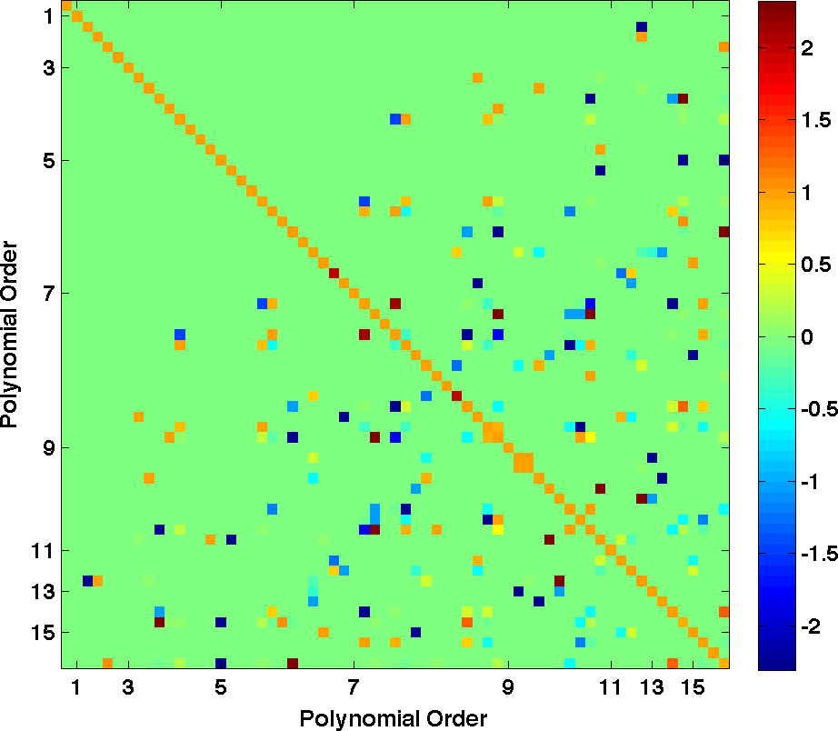
We will see in the numerical results in the next section that – across all test cases – the pseudospectral coefficients corresponding to the higher order polynomials are inaccurate when computed directly with the sparse grid integration rule. This occurs because the higher order basis functions are not orthonormal with respect to the sparse grid quadrature rule. However, when the integrations are performed using the SPAM, the basis polynomials are orthonormal. This becomes apparent by looking at the SPAM coefficients for each basis polynomial in the set $\Pi$ from (41).

Theorem 2.

Let $f(s)=\phi(s)$ for some $\phi(s)\in\Pi$ from (41). Then

$$\hat{f}_{\pi}=\left\{\begin{array}[]{cl}1&\mbox{ if $\pi(s)=\phi(s)$,}\\ 0&\mbox{ otherwise,}\end{array}\right.$$ (45)

where $\hat{f}_{\pi}$ is from (43).

Proof.

Using Proposition 3 from [8], we have $\mathcal{A}_{p}(f)=f$ for $f=\phi\in\Pi$, which implies that $\mathcal{A}_{p}$ is a projector for the polynomial space defined by $\mathrm{span}\,(\Pi)$. Noting that the elements of $\Pi$ are linearly independent completes the proof. ∎

Figure 1a numerically verifies the orthonormality of the elements of $\Pi$ using the SPAM; Figure 1b demonstrates the loss of orthonormality for the higher order elements of $\Pi$ for a discrete inner product defined by the points and weights of the sparse grid integration rule. We use $d=2$ and $l=4$, and we order the basis polynomials by their degree. Notice that some of the lower order basis polynomials are orthonormal with respect to a discrete norm defined by the sparse grid quadrature rule. This is due to the degree of exactness of the sparse grid quadrature rule; see [24] for more details.

(a) SPAM

(b) Sparse grid integration

Figure 1: Orthonormality of the elements in $\Pi$ from (41) using SPAM or directly approximated with the sparse grid integration rule with dimension $d=2$ and level $l=4$. The sparse grid was built from univariate Gauss-Legendre quadrature rules with growth rule (34).

4 Numerical Experiments

In the following numerical experiments, we compare the coefficients computed with the SPAM to direct approximation of the Fourier coefficients with the corresponding sparse grid quadrature rule. To make the comparison fair, we apply the sparse grid rule directly to each coefficient corresponding to the basis set (41) for the sparse pseudospectral approximation. We construct each sparse grid rule using (i) univariate non-nested Gauss-Legendre quadrature points for a uniform weight function on the square $[-1,1]^{2}$, (ii) $n_{m}$ defined as in (34), and (iii) $\mathcal{I}$ and $c(\mathbf{m})$ defined as in (36) and (37). The choice of the uniform weight function implies the $\pi_{i}(s)$ are the normalized Legendre polynomials for the pseudospectral approximation. For all experiments, we compute the largest feasible tensor product pseudospectral approximation and call the resulting coefficients the truth. In all cases, the apparent decay in the tensor product pseudospectral coefficients assures us that we have used a sufficiently high order approximation to bestow the title truth.

4.1 Five Bivariate functions

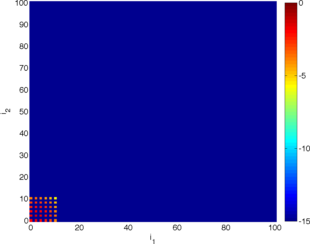
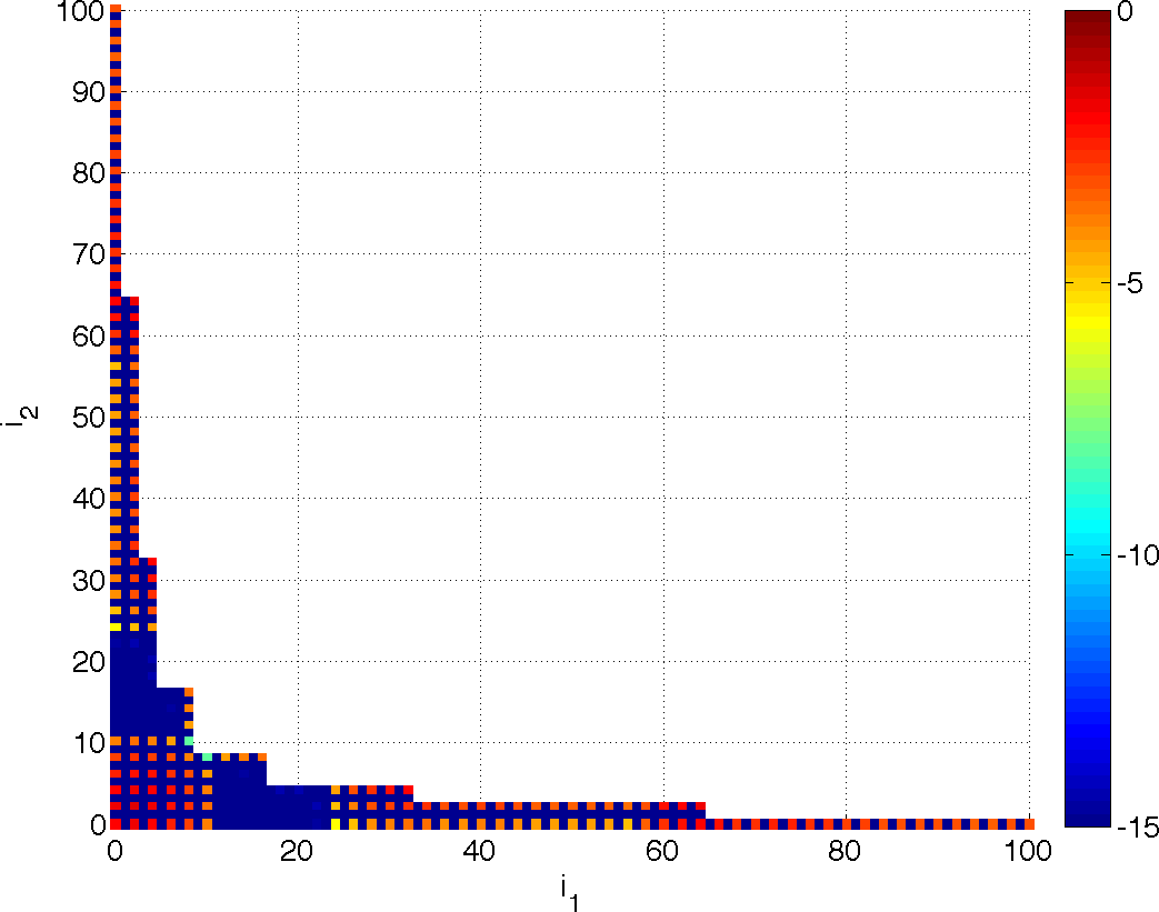
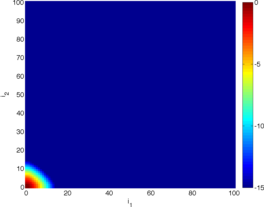
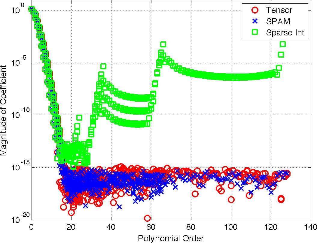
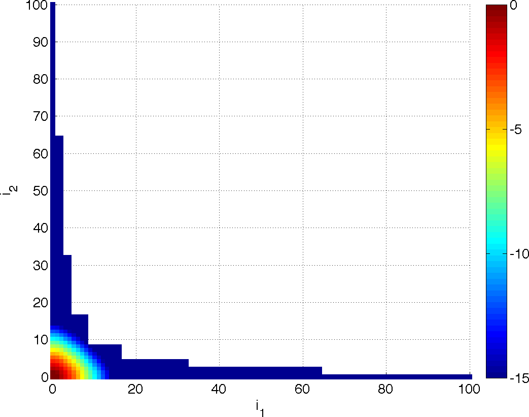
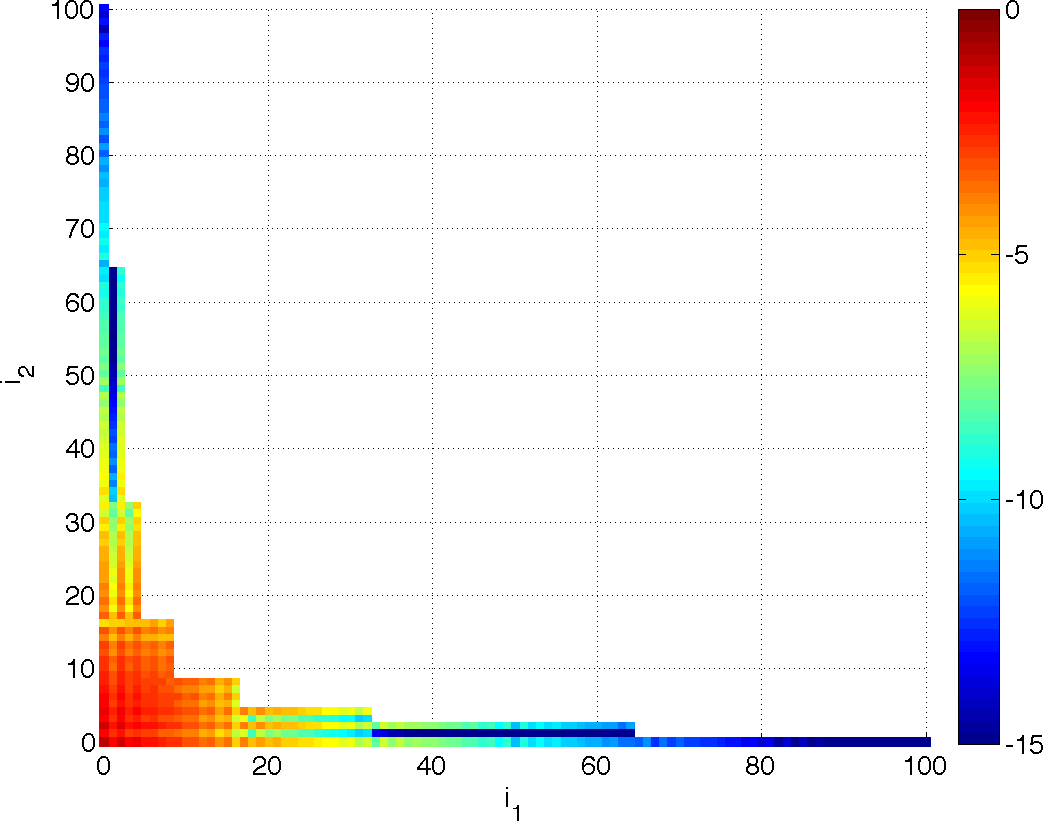
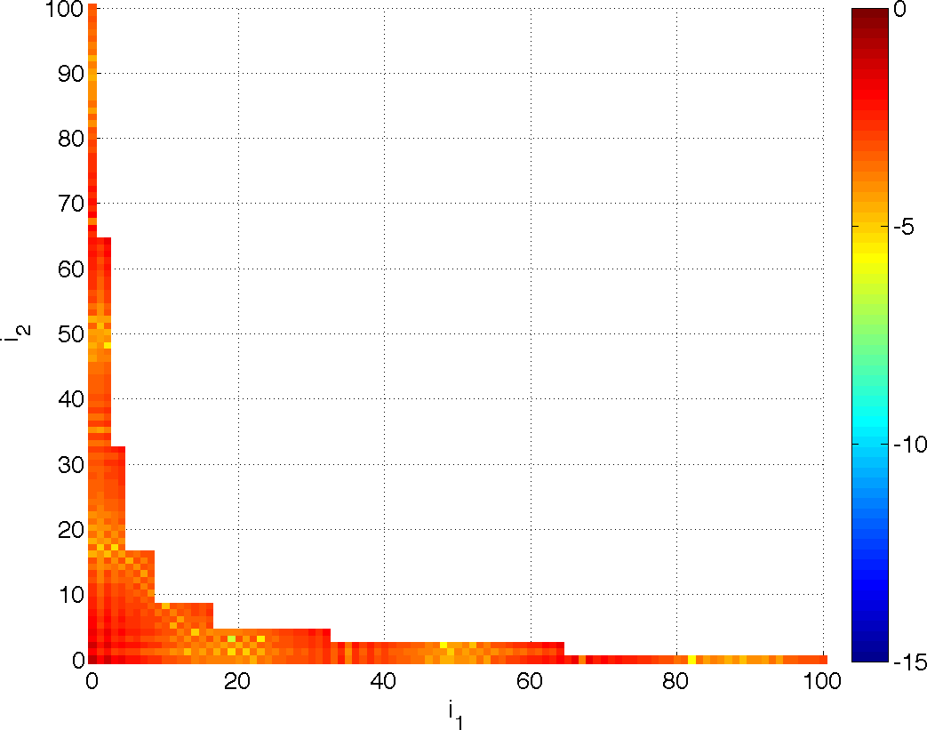
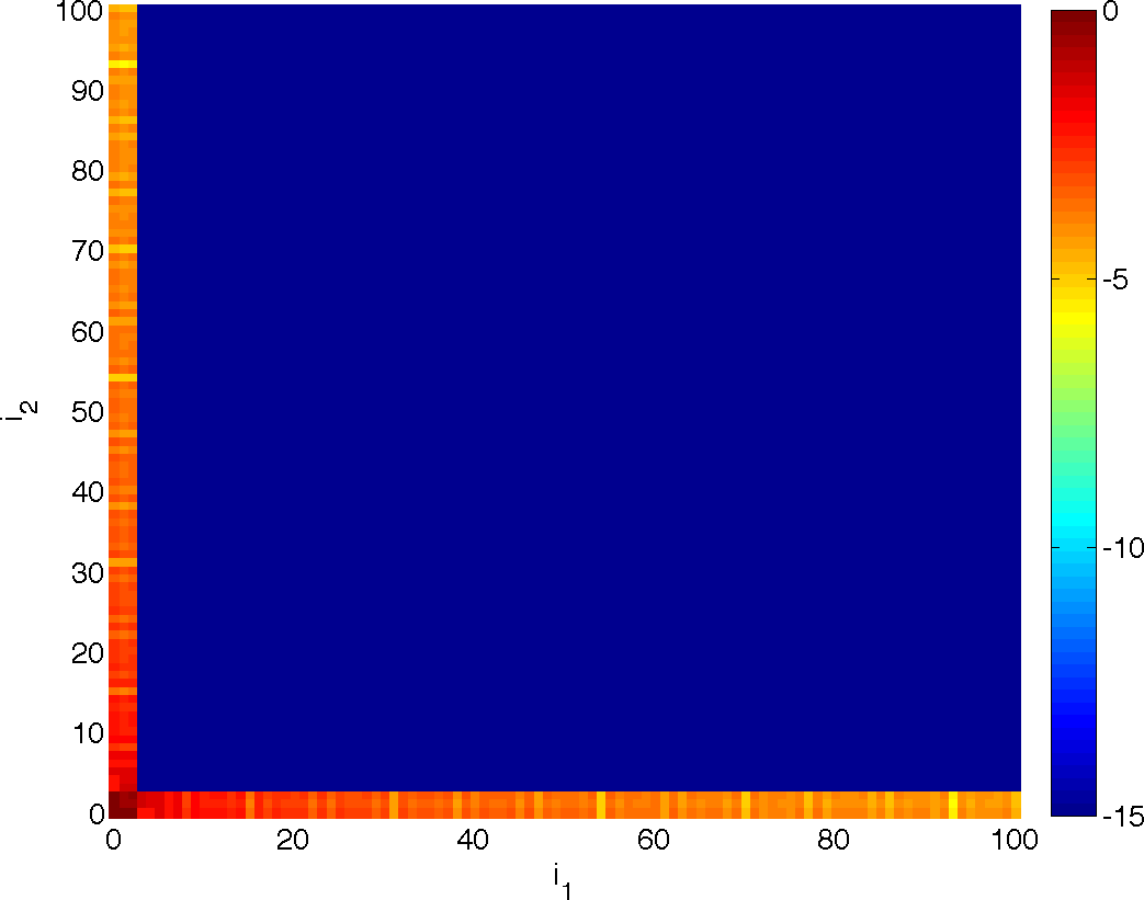
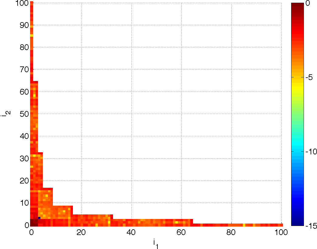
In the first experiment, we compare both methods on five bivariate functions; see Table 1. For each function, we compute a tensor product pseudospectral approximation of order 255 in each variable – 65,536 total quadrature points. We plot the log of the magnitude of the pseudospectral coefficients with a surface plot to visually observe their decay. We then plot the log of the magnitude of the sparse pseudospectral coefficients corresponding to a level $l=7$ sparse grid compared to the same sparse grid approximation of the Fourier coefficients.

#	$f(s_{1},s_{2})$
1	$s_{1}^{10}s_{2}^{10}$
2	$e^{s_{1}+s_{2}}$
3	$\sin(5(s_{1}-0.5))+\cos(3(s_{2}-1))$
4	$1/(2+16(s_{1}-0.1)^{2}+25(s_{2}+0.1)^{2})$
5	$(|s_{1}-0.2|+|s_{2}+0.2|)^{3}$

Table 1: The five bivariate test functions.

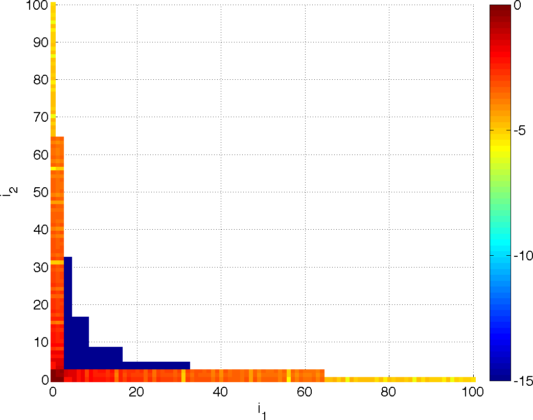
With a level 7 grid, sparse pseudospectral approximation contains a maximum univariate degree of 129. For each test function, the corresponding set of figures contains

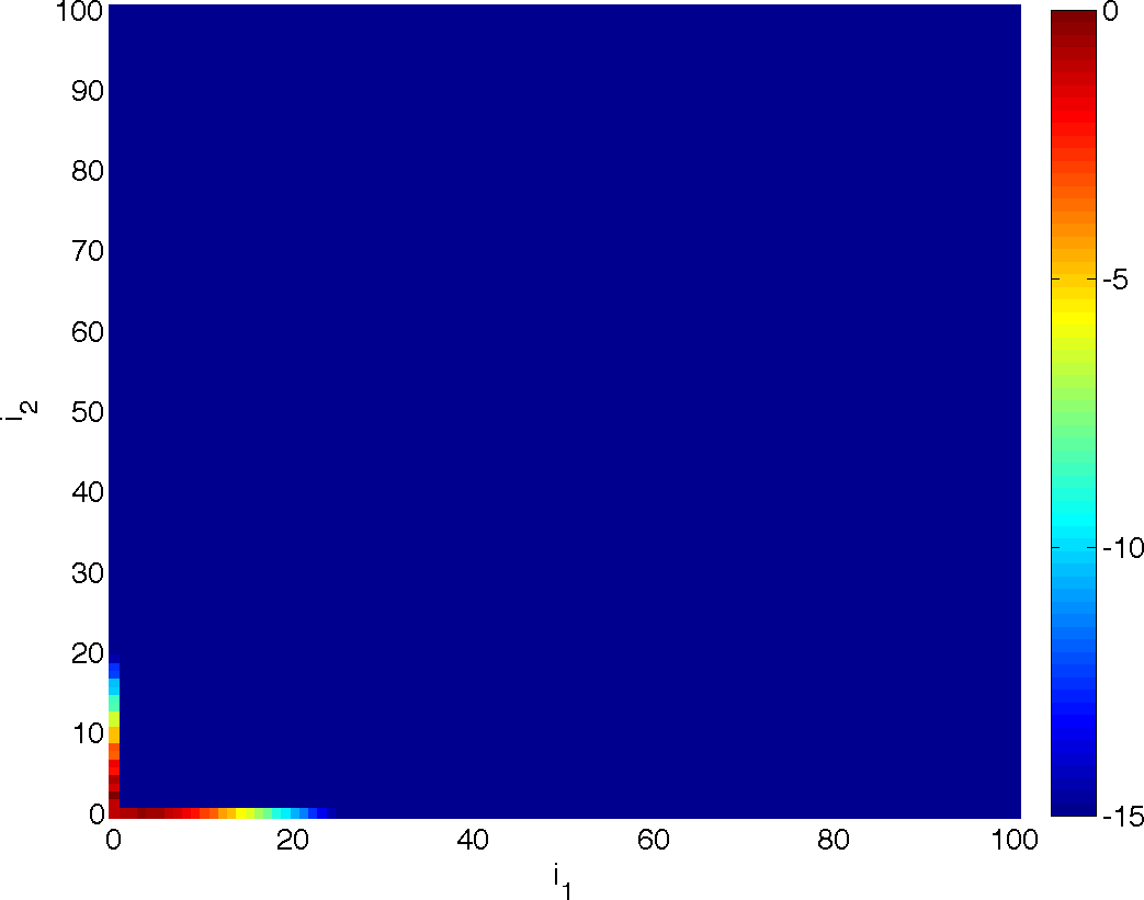
1. the tensor product pseudospectral coefficients up to maximum univariate degree 100,

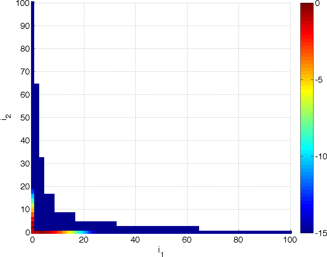
2. the SPAM coefficients up to maximum univariate degree 100,

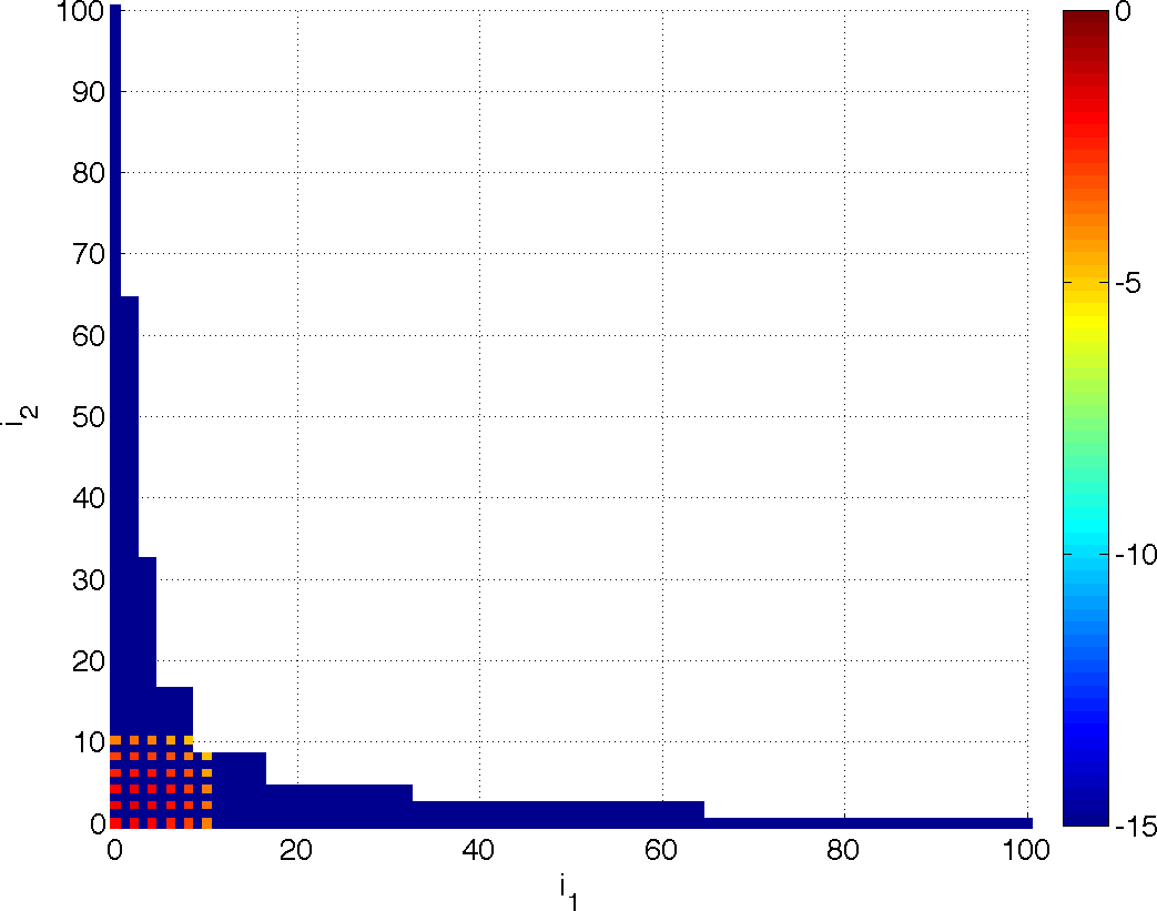
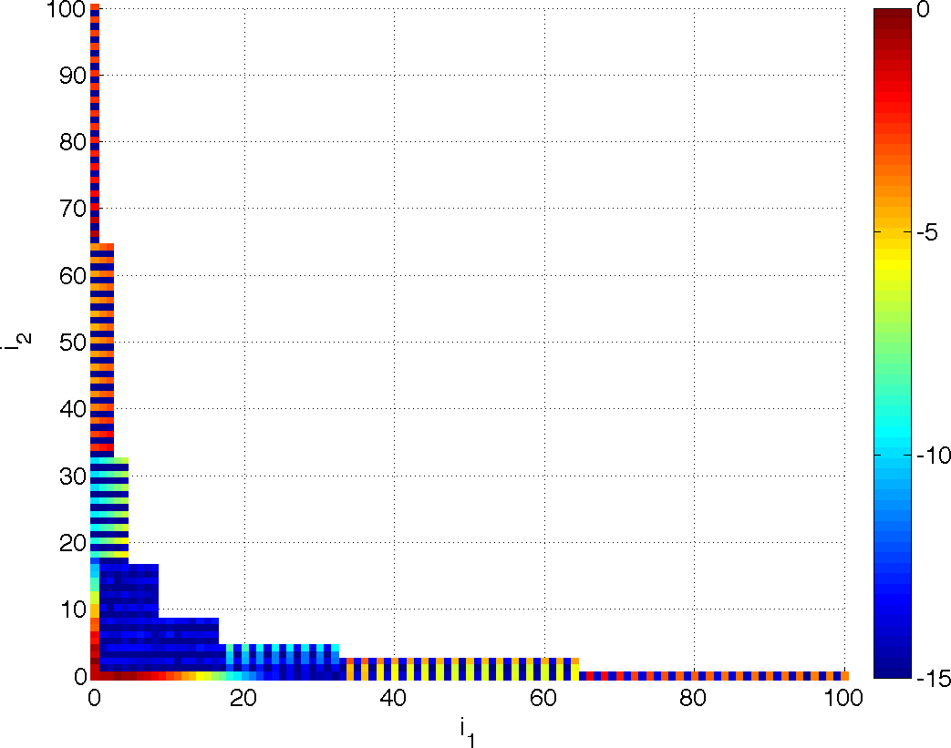
3. the sparse grid integration approximation of the Fourier coefficients up to maximum univariate degree 100,

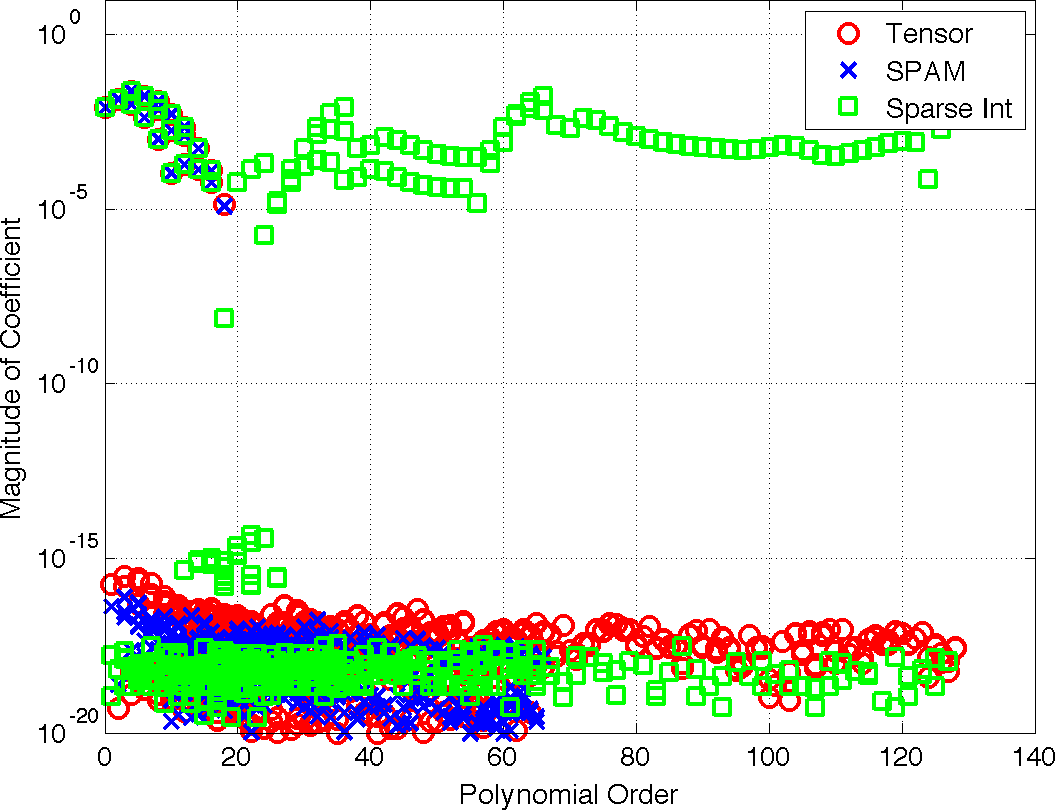
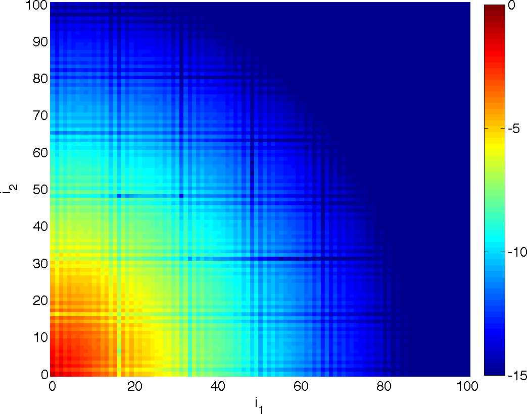
4. a summary plot with coefficients up to univariate degree 129 ordered by total order.

As a general comment, we see that the sparse grid integration produces largely incorrect values for coefficients associated with higher degree polynomials. More specific comments for the individual test functions are as follows:

1. $s_{1}^{10}s_{2}^{10}$: This function evaluates the performance of the methods on a monomial. We know that coefficients associated with polynomials of degree greater than 10 in either $s_{1}$ or $s_{2}$ should be zero by orthogonality. Additionally, since the monomial is an even function over the domain with a symmetric weight function, the coefficients corresponding to odd degree polynomials in either variable ought to be zero. This is verified in the tensor product pseudospectral coefficients and respected by the SPAM coefficients. However, the direct sparse integration produces non-zero values for coefficients that should be zero. See Figure 2.

2. $e^{s_{1}+s_{2}}$: This function is analytic in both variables with rapid decay of the Fourier coefficients. Observe that the direct sparse integration yields large values for coefficients corresponding to the higher order polynomials. See Figure 3.

3. $\sin(5(s_{1}-0.5))+\cos(3(s_{2}-1))$: In the language of the ANOVA decomposition [25], this function has only main effects. Thus, the Fourier coefficients for polynomials with mixed terms corresponding to interaction effects should be zero. Again, this is apparent in the tensor product pseudospectral coefficients, and it is respected by the SPAM coefficients. The direct sparse integration, however, produces non-zero values for coefficients of the mixed polynomials; see Figure 4.

4. $1/(2+16(s_{1}-0.1)^{2}+25(s_{2}+0.1)^{2})$: The pseudospectral coefficients of this rational function decay relatively slowly; notice it needs up to degree 40 polynomials in each variable to reach numerical precision, according to the tensor product pseudospectral coefficients. The SPAM coefficients do a much better job capturing the true decay of the Fourier coefficients than the direct integration method, which does not appear to decay at all. See Figure 5.

5. $(|s_{1}-0.2|+|s_{2}+0.2|)^{3}$: This function has discontinuous first derivatives, so we expect only first order algebraic convergence of its Fourier coefficients; on a log scale they decay very slowly. However, the interaction effects disappear after degree three in either variable. Again, this is visible in the tensor product pseudospectral coefficients and respected by the SPAM coefficients, but the direct sparse grid integration produces non-zero values for coefficients that ought to be zero. See Figure 6.

In general, we find that the SPAM coefficients are significantly more accurate than the direct application of the sparse grid integration rules to the Fourier coefficients. This observation is somewhat counterintuitive. One may expect that the sparse grid rule, by evaluating the product of the function times the basis polynomial at more locations, would yield a more accurate approximation. But this is clearly not the case for these examples. The decreased accuracy in the coefficients computed with the sparse grid integration rule is a result of the nonorthogonality of the basis polynomials with respect to a discrete inner product defined by the sparse grid integration rule; see Section 3.1.

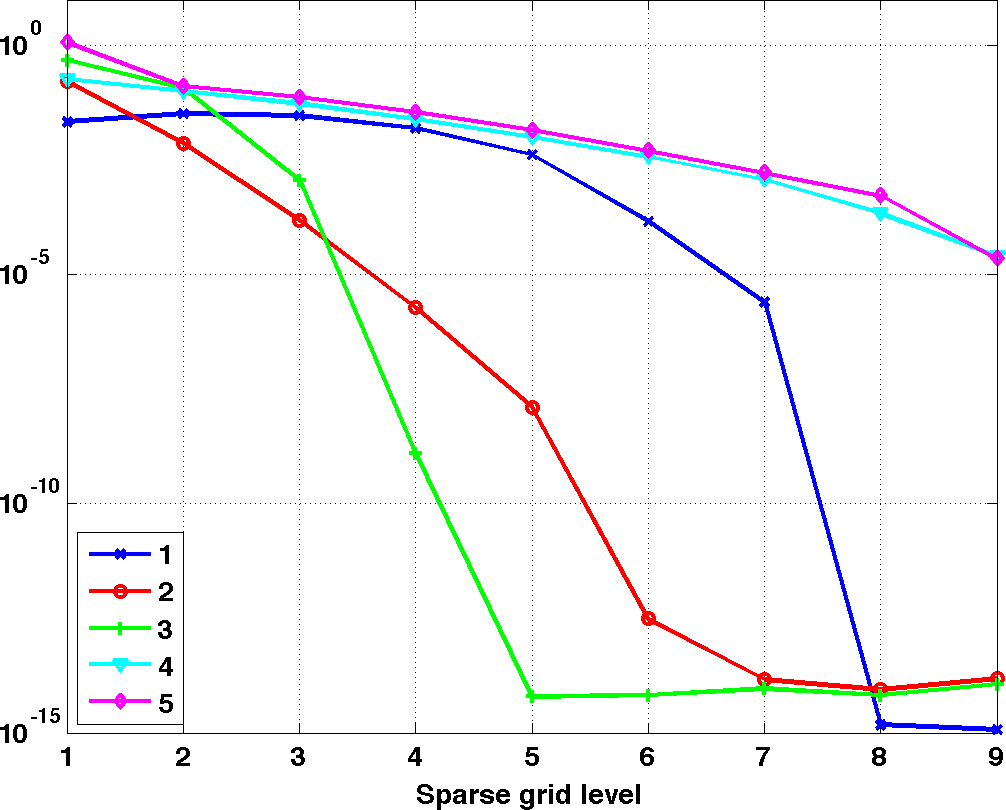
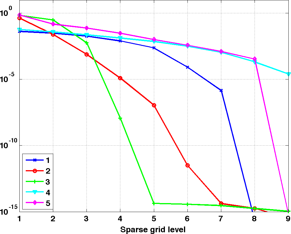
In Figure 7c, we plot the decay of the truncation error for the sparse approximations as the level increases. We approximate the truncation error by the sum of squares of the neglected coefficients from the tensor product expansion. Since both approximations use the same basis sets, this approximate truncation error is identical. In Figures 7a and 7b we plot the decay in the error of the approximated coefficients as the level increases; the error in the coefficients is squared and summed. We see that the error in the SPAM coefficients decays roughly like the truncation error, while the error in the direct sparse grid integration does not decay. Of course, this summary plot ignores what is most visible in Figures 2-6, which is that some of the coefficients associated with lower order polynomials may be approximated well; it is the coefficients of the higher order terms that contain most of the error.

(a) Tensor $100\times 100$

(b) Coefficient decay

(c) SPAM

(d) Sparse grid integration

Figure 2: Fourier coefficient approximations for $s_{1}^{10}s_{2}^{10}$.

(a) Tensor $100\times 100$

(b) Coefficient decay

(c) SPAM

(d) Sparse grid integration

Figure 3: Fourier coefficient approximations for $e^{s_{1}+s_{2}}$.

(a) Tensor $100\times 100$

(b) Coefficient decay

(c) SPAM

(d) Sparse grid integration

Figure 4: Fourier coefficient approximations for $\sin(5(s_{1}-0.5))+\cos(3(s_{2}-1))$.

(a) Tensor $100\times 100$

(b) Coefficient decay

(c) SPAM

(d) Sparse grid integration

Figure 5: Fourier coefficient approximations for $1/(2+16(s_{1}-0.1)^{2}+25(s_{2}+0.1)^{2})$.

(a) Tensor $100\times 100$

(b) Coefficient decay

(c) SPAM

(d) Sparse grid integration

Figure 6: Fourier coefficient approximations for $(|s_{1}-0.2|+|s_{2}+0.2|)^{3}$.

(a) SPAM coefficient error

(b) Sparse grid integration coefficient error

(c) Truncation error

Figure 7: Comparison of truncation error to error coefficient approximation between SPAM and direct sparse grid integration for each of the five test functions, numbered according to Table 1.

4.2 PDE with Random Input Data

The last numerical example we examine is a linear elliptic diffusion equation with a stochastic diffusion coefficient. Let $D=[0,1]\times[0,1]$ and $(\Omega,\mathcal{B},P)$ be a complete probability space. We seek the function $u:D\times\Omega\rightarrow\mathbb{R}$ such that the following holds $P$-a.e.:

$$\begin{split}-\nabla\cdot(a(x,\omega)\nabla u(x,\omega))&=1,\quad x\in D,\\ u(x)&=0,\quad x\in\partial D.\end{split}$$ (46)

Instead of the whole solution $u$, we are interested in computing the response function

$$g(\omega)=\int_{D}u(x,\omega)dx$$ (47)

which is the spatial mean of $u$ over $D$.

The diffusion coefficient $a(x,\omega)$ is modeled as a random field with exponential correlation:

$$C(x,y)\equiv E[a(x,\omega)a(y,\omega)]=\sigma^{2}e^{\|x-y\|_{1}/L}$$ (48)

where $\sigma=0.1$ is the standard deviation of the field and $L=1$ is the correlation length. It is approximated through a truncated Karhunen-Loéve expansion [26]:

$$a(x,\omega)\;\approx\;\hat{a}_{d}(x,s(\omega))\;=\;a_{0}(x)\,+\,\sum_{k=1}^{d}\sqrt{\lambda_{k}}a_{k}(x)\,s_{k}(\omega),$$ (49)

where $a_{0}(x)=\mu=0.2$ is the mean of the random field, $(\lambda_{k},a_{k}(x))$, $k=1,\dots,d$ are eigenvalue-eigenfunction pairs for the covariance operator:

$$\int_{D}C(x,y)a_{k}(x)dx=\lambda_{k}a_{k}(y),\quad y\in D,$$ (50)

and $s=(s_{1},\dots,s_{d})$ are uncorrelated, uniform random variables on $[-1,1]$. We make the further modeling assumption that the random variables are independent. Define $\Gamma=[-1,1]^{d}$ to be the range of $s$ and

$$w(s)=\left\{\begin{array}[]{cl}1/2^{d}&s\in[-1,1]^{d}\\ 0&\mbox{ otherwise}\end{array}\right.$$ (51)

to be the density of $s$. The eigenvalues and eigenfunctions are computed using a pseudo-analytic procedure described in [2]. The eigenvalues are sorted in decreasing order, and we use the first $d=5$ eigenvalues/eigenfunctions to approximate the random field.

Let $\pi_{i}:[-1,1]\rightarrow\mathbb{R}$, $i=1,2,\dots$ be the normalized Legendre polynomial of order $i-1$. For a given multi-index $\mathbf{i}=(i_{1},\dots,i_{d})$, define the tensor product polynomial

$$\pi_{\mathbf{i}}(s)=\pi_{i_{1}}(s_{1})\dots\pi_{i_{d}}(s_{d}).$$ (52)

Given a set $\mathcal{I}$ of multi-indices, we approximate $g(\omega)$ by

$$\hat{g}(\omega)=\sum_{\mathbf{i}\in\mathcal{I}}\hat{g}_{\mathbf{i}}\pi_{\mathbf{i}}(s(\omega))$$ (53)

where the unknown coefficients $\hat{g}_{\mathbf{i}}$ are computed through pseudospectral projection using both SPAM and sparse grid integration. For a given $s$, the corresponding response $g$ is computed by solving

$$\begin{split}-\nabla\cdot(\hat{a}_{d}(x,s)\nabla u(x)&=1,\quad x\in D,\\ u(x)&=0,\quad x\in\partial D,\\ g&=\int_{D}u(x)dx.\end{split}$$ (54)

These equations are discretized using piecewise linear finite elements over quadrilateral mesh cells of size $1/512$, which gave a spatial error of $\mathcal{O}(10^{-6})$. The resulting linear algebraic equations are solved via preconditioned GMRES using an algebraic multigrid preconditioner with tolerance of $10^{-12}$. The finite element equations were implemented and solved using a variety of packages within the Trilinos solver framework [27]. The resulting SPAM and sparse grid integrations were provided by the Dakota package [28].

Note that instead of using the growth relationship in (34), we choose

$$n_{m}=2m-1,\quad m\geq 1.$$ (55)

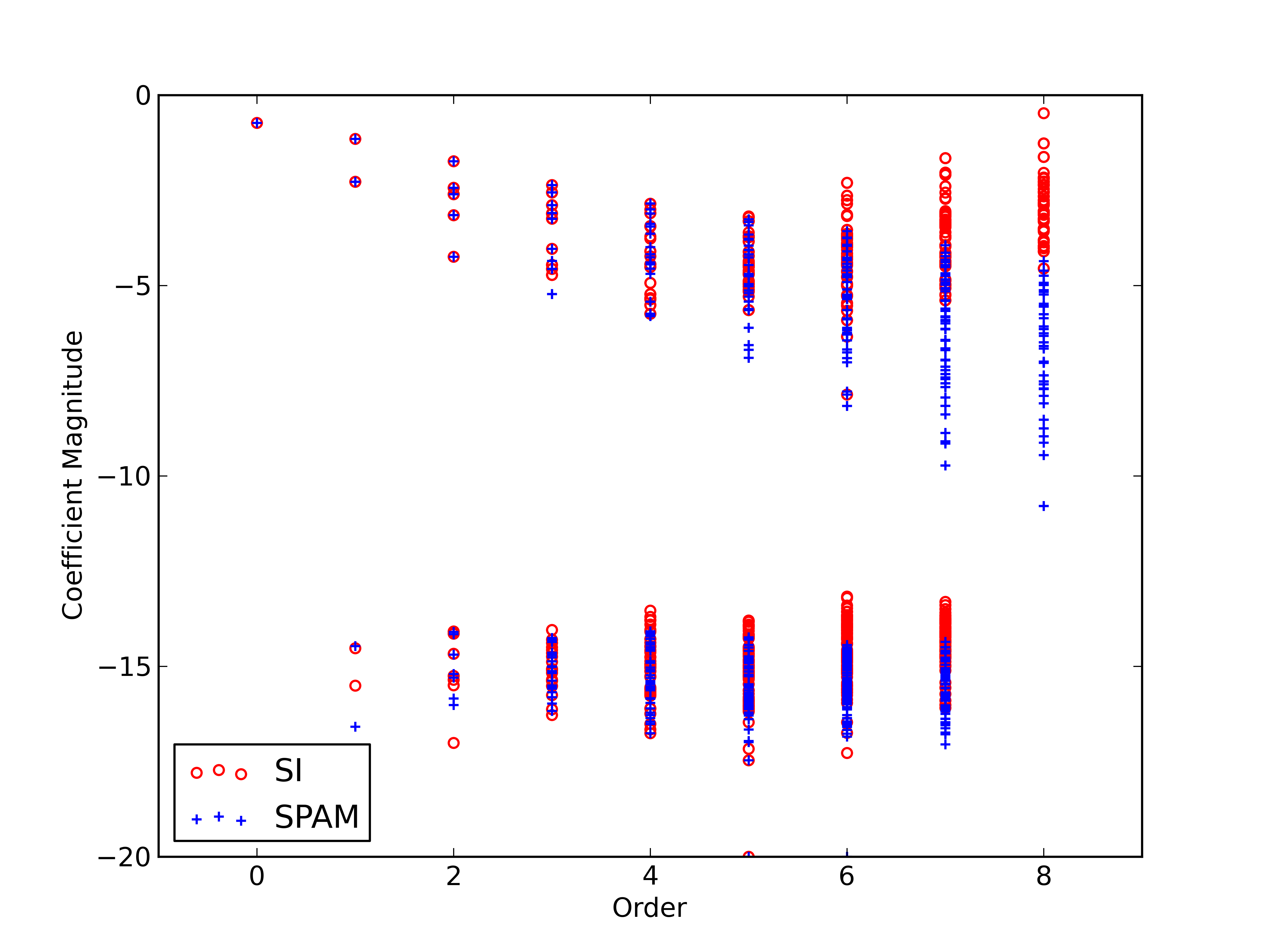
This growth relationship yields tensor grids with many fewer points compared to (34). The multiplication factor $2$ ensures that all tensor grids will share the mid-point of the domain, which reduces the total number of function evaluations. The corresponding coefficients of the stochastic response function $g$ are plotted in Figure 8 by the degree of the corresponding multivariate polynomial. The level parameter for the sparse grid is 4.

One can see as the order of the polynomials increases, the coefficients generated by SPAM decay as they should, whereas those generated through direct sparse integration begin to diverge for the higher order polynomials. Note, however, that the difference is not as pronounced compared to the bivariate test cases. We attribute this to the use of the growth relationship (55), as opposed to (34) used with the bivariate functions.

Figure 8: Comparison of approximate Fourier coefficients of the stochastic response (53) of the linear diffusion problem (46) using SPAM and sparse integration for dimension $d=5$ and level $l=4$. The figure plots the coefficients according to the degree of associated polynomial.

5 Conclusions

Sparse grid integration rules are constructed as linear combinations of tensor product quadrature rules. By taking advantage of the equivalence between the tensor product Lagrange interpolant and a pseudospectral approximation with a tensor product orthogonal polynomial basis, we can linearly combine the tensor product polynomial expansions associated with each tensor grid quadrature rule to produce a sparse pseudospectral approximation. We have numerically compared this approach to direct sparse grid integration of the Fourier coefficients. The experiments show convincingly that the direct integration approach produces inaccurate approximations of the Fourier coefficients associated with the higher order polynomial basis functions, while the SPAM coefficients are much more accurate.

The difference between SPAM and the sparse grid integration of the Fourier coefficients is present in all Smolyak type approximations – including anisotropic and adaptive variants. While not presented explicitly in this paper due to space limitations, the authors have conducted similar studies on such variants with similar results. The conclusions are clear. Given a function evaluated at the nodes of a sparse grid integration rule, the proper way to approximate the Fourier coefficients of an orthogonal expansion is the SPAM.

References

- [1] D. Xiu, G. E. Karniadakis, The Wiener-Askey polynomial chaos for stochastic differential equations, SIAM Journal of Scientific Computing 24 (2002) 619 – 644.
- [2] R. Ghanem, P. D. Spanos, Stochastic Finite Elements: A Spectral Approach, Springer-Verlag, New York, 1991.
- [3] D. Xiu, J. S. Hesthaven, High order collocation methods for differential equations with random inputs, SIAM Journal of Scientific Computing 27 (2005) 1118 – 1139.
- [4] I. Babus̆ka, F. Nobile, R. Tempone, A stochastic collocation method for elliptic partial differential equations with random input data, SIAM Journal of Numerical Analysis 45 (2007) 1005 – 1034.
- [5] H.-J. Bungartz, M. Griebel, Sparse grids, Acta Numerica (2004) 147–269.
- [6] E. Novak, K. Ritter, High dimensional integration of smooth functions over cubes, Numerische Mathematik 75 (1) (1996) 79–97.
- [7] F. Nobile, R. Tempone, C. G. Webster, A sparse grid stochastic collocation method for partial differential equations with random input data, SIAM Journal of Numerical Analysis 46 (2008) 2309 – 2345.
- [8] V. Barthelmann, E. Novak, K. Ritter, High dimensional polynomial interpolation on sparse grids, Advances in Computer Mathematics 12 (2000) 273–288.
- [9] G. Szegö, Orthogonal Polynomials, American Mathematical Society, Providence, RI, 1939.
- [10] C. F. Dunkl, Y. Xu, Orthogonal Polynomials in Several Variables, Cambridge University Press, 2001.
- [11] D. Xiu, Efficient collocational approach for parametric uncertainty analysis, COMMUNICATIONS IN COMPUTATIONAL PHYSICS 2 (2) (2007) 293–309.
-
[12]
O. P. L. Maitre, M. T. Reagan, H. N. Najm, R. G. Ghanem, O. M. Knio,
A
stochastic projection method for fluid flow: Ii. random process, Journal of
Computational Physics 181 (1) (2002) 9 – 44.
doi:DOI:10.1006/jcph.2002.7104.
URL http://www.sciencedirect.com/science/article/pii/S00219%99102971044 -
[13]
M. T. Reagan, H. N. Najm, R. G. Ghanem, O. M. Knio,
Uncertainty quantification in reacting-flow simulations through non-intrusive
spectral projection, Combustion and Flame 132 (3) (2003) 545 – 555.
doi:DOI:10.1016/S0010-2180(02)00503-5.
URL http://www.sciencedirect.com/science/article/pii/S00102%18002005035 - [14] M. S. Eldred, C. G. Webster, P. G. Constantine, Evaluation of non-intrusive approaches for Wiener-Askey generalized polynomial chaos, AIAA Paper (2008-1892).
- [15] J. Shen, L.-L. Wang, Sparse spectral approximations of high-dimensional problems based on hyperbolic cross, SIAM Journal of Numerical Analysis 48 (2010) 1087–1109.
- [16] J. Shen, H. Yu, Efficient spectral sparse grid methods and applications to high-dimensional elliptic problems, SIAM J. Sci. Comput. 32 (2010) 3228–3250.
- [17] W. Gautschi, Orthogonal Polynomials: Computation and Approximation, Clarendon Press, Oxford, 2004.
- [18] L. N. Trefethen, Is Gauss quadrature better than Clenshaw-Curtis?, SIAM Review 50 (2008) 67–87.
- [19] S. Smolyak, Quadrature and interpolation formulas for tensor products of certain classes of function, Soviet Math. Dokl. 4 (1963) 240–143.
- [20] T. N. L. Patterson, The optimum addition of points to quadrature formulae, Mathematics of Computation 22 (1968) 847–856.
- [21] C. W. Clenshaw, A. R. Curtis, A method for numerical integration on an automatic computer, Numerische Mathematik 2 (1960) 197–205.
- [22] F. Nobile, R. Tempone, C. G. Webster, An anisotropic sparse grid stochastic collocation method for partial differential equations with random input data, SIAM Journal of Numerical Analysis 46 (2008) 2411–2442.
- [23] T. Gerstner, M. Griebel, Numerical integration using sparse grids, Numerical Algorithms 18 (1998) 209–232.
[24]
E. Novak, K. Ritter, Simple
cubature formulas with high polynomial exactness, Constructive Approximation
15 (1999) 499–522, 10.1007/s003659900119.
URL http://dx.doi.org/10.1007/s003659900119 - [25] R. Liu, A. B. Owen, Estimating mean dimensionality of analysis of variance decompositions, Journal of the American Statistical Association 101 (2006) 712–721.
- [26] M. Loève, Probability Theory II, Springer-Verlag, 1978.
- [27] M. Heroux, R. Bartlett, V. Howle, R. Hoekstra, J. Hu, T. Kolda, R. Lehoucq, K. Long, R. Pawlowski, E. Phipps, A. Salinger, H. Thornquist, R. Tuminaro, J. Willenbring, A. Williams, K. Stanley, An overview of the Trilinos package, ACM Trans. Math. Softw. 31 (3), http://trilinos.sandia.gov/.
- [28] M. S. Eldred, B. M. Adams, D. M. Gay, L. P. Swiler, K. Haskell, W. J. Bohnhoff, J. P. Eddy, W. E. Hart, J.-P. Watson, P. D. Hough, T. G. Kolda, DAKOTA, a multilevel parallel object-oriented framework for design optimization, parameter estimation, uncertainty quantification, and sensitivity analysis, Tech. Rep. SAND2006-6337, Sandia National Laboratories (2006).