Uncharged compactlike and fractional Lorentz-violating BPS vortices in the CPT-even sector of the standard model extension

Abstract

We have investigated and verified the existence of stable uncharged Bogomol’nyi-Prasad-Sommerfeld (BPS) vortices in the framework of an Abelian Maxwell-Higgs model supplemented with CPT-even and Lorentz-violating (LV) terms belonging to the gauge and Higgs sectors of the standard model extension. The analysis is performed in two situations: first, one by considering the Lorentz violation only in the gauge sector and then in both gauge and Higgs sectors. In the first case, it is observed that the model supports vortices somehow equivalent to the ones appearing in a dielectric medium. The Lorentz violation controls the radial extension (core of the solution) and the magnetic field amplitude of the Abrikosov-Nielsen-Olesen vortices, yielding compactlike defects in an alternative and simpler way than that of $k-$field models. At the end, we consider the Lorentz-violating terms in the gauge and Higgs sectors. It is shown that the full model also supports compactlike uncharged BPS vortices in a modified vacuum, but this time there are two LV parameters controlling the defect structure. Moreover, an interesting novelty is introduced by the LV-Higgs sector: fractional vortex solutions.

I
Introduction

The investigation of stable vortex configurations has been an issue of permanent interest since the pioneering proposal of Abrikosov-Nielsen-Olesen (ANO) ANO . In the early 1990s, vortex configurations were analyzed in the context of planar theories including the Chern-Simons term CS , which provided the possibility of having charged vortices CSV . The Chern-Simons vortex configurations support Bogomol’nyi-Prasad-Sommerfeld (BPS) solutions and present important connections with the physics of anyons and the fractional quantum Hall effect Ezawa . The Chern-Simons vortices were studied with nonminimal coupling CSV1 , and they remain a topic of intensive investigation with recent developments CSV2 ; Bolog . Generalized Chern-Simons vortex solutions were recently examined in the presence of a noncanonical kinetic term Hora1 and k-field terms (high-order derivative terms) Compact1 . Generalized vortex solutions were also attained in the contexts of the Abelian Maxwell-Higgs (AMH) model Hora1b and twinlike models HoraTwin . The k-field theories work with nonlinear functions of the usual kinetic term to obtain new solutions for nonlinear systems, with interesting applications in cosmology and inflation Cosmology , dark matter DM , tachyon matter Tachyon , ghost condensates GC and topological defects kfield . Concerning topological defects, the higher-order kinetic terms engender the formation of k-defects (compactlike solutions), structures whose core can be much smaller than the one of the usual solutions kfield ; Hora2 ; Hora3 . When a k-defect presents a compact support, it is dubbed a compacton Compact2 ; Compact3 . In the present work, we show that the inclusion into the AMH model of Lorentz-violating (LV) terms-belonging to the theoretical framework of the standard model extension (SME)- can yield compactlike vortex solutions and also fractional quantization of the magnetic flux.

Lorentz symmetry violation has been much investigated in the past few years, having as a theoretical framework the standard model extension Colladay , based on the idea of a spontaneous Lorentz-symmetry breaking in a theory defined at the Planck scale Samuel . The SME incorporates LV terms, generated as non-null vacuum expectation values of Lorentz tensors, in all sectors of the standard model. The investigations in the context of the SME concern mainly the fermion sector Fermion ; Fermion2 ; Fermion3 , extensions involving gravity Gravity ,Gravity2 , and the gauge sector Jackiw -Klink3 . The gauge sector of the SME is composed of a CPT-odd part (the Carroll-Field-Jackiw term Jackiw ) and a CPT-even part, which is represented by the tensor $\left(k_{F}\right)_{\mu\nu\alpha\beta}.$ The electrodynamics modified by this term has been investigated since 2002, with a twofold purpose: to scrutinize the new physical properties induced by its 19 Lorentz-violating coefficients and to impose tight upper bounds on the magnitude of these coefficients.  The CPT-even tensor $\left(k_{F}\right)_{\mu\nu\alpha\beta}$ has the same symmetries as the Riemann tensor, and a double null trace, $\left(k_{F}\right)^{\mu\nu}{}_{\mu\nu}=0$. References. KM1 ; KM2 , stipulated the existence of 10 components sensitive to birefringence and 9 that are called nonbirefringent. The 10 birefringent components are severely constrained to the level of $1$ part in $10^{32}$ by spectropolarimetry data of cosmological sources KM1 ; KM2 . The nonbirefringent coefficients are constrained by other tests, involving the study of Cherenkov radiation Cherenkov2 , the absence of emission of Cherenkov radiation by ultrahigh energy cosmic rays Klink2 ; Klink3 , and the subleading birefringent behavior of the nonbirefringent parameters Qasem , able to yield upper bounds of up to $1$ part in $10^{37}$ on these coefficients. The gauge sector of the SME has also been investigated in the context of arbitrary dimensional operators Kostelec .

Effects of Lorentz violation on topological defects have been investigated in distinct scenarios. Some works have examined the role played by Lorentz-violating terms on defects defined in the framework of scalar systems Defects , revealing the associated properties and preservation of the linear stability. In another line, the existence of monopole solutions in the presence of the Lorentz-violating Carroll-Field-Jackiw term was first studied in Ref. Monopole1 . Recently, the existence of monopoles in the framework of a rank-2 antisymmetric Kalb-Ramond tensor field, generated in a spontaneous symmetry breaking, was analyzed in Ref. Monopole2 , unveiling some similarities between the profiles of the antisymmetric Kalb-Ramond monopole and the usual O(3) one. A more complete study of topological defects in the context of field theories endowed with a tensor which spontaneously breaks Lorentz symmetry was accomplished in Ref. Seifert . Up the moment, there is no report of works investigating vortex solutions in the presence of Lorentz-violating terms, except for a preliminary contribution Baeta2 . There are some addressing vortex configurations in noncommutative scenarios which yield Lorentz symmetry only as a by-product Gamboa .

In this work, we investigate for the first time the formation of stable uncharged vortex configurations in the context of a Lorentz-violating and CPT-even AMH electrodynamics in two situations: (i) with a Lorentz-violating term only in the gauge sector, and (ii) introducing Lorentz-violating terms simultaneously in the gauge and Higgs sectors of the model. In both cases the Higgs sector is endowed with a particular and appropriated fourth-order self-interacting potential. In the first case, one verifies the existence of BPS solutions, governed by analogue equations to the AMH model. The Lorentz-violating parameter appears as a key element for defining an effective electrical coupling constant and modifying the mass of the boson fields. The vortex profiles, generated by numerical methods, reveal that the Lorentz- violating parameter acts as an element able to control the radial extension of the defect (vortex core), in a similar way as observed in k-field theories which engender compactlike structures. Finally, in order to address a more complete Lorentz-violating framework supporting vortex solutions, we consider the AMH model with two CPT-even Lorentz-violating terms in the Higgs sector as well. We achieve the equations of motion and evaluate the fourth-order potential (compatible with the BPS solutions), which entails two vacua. After showing that the Higgs LV parameter induces energy instability, we find the self-interacting potential (endowed with only one vacuum) and BPS equations for the stable uncharged vortices. We finally demonstrate that the asymptotic solutions are only compatible with a modified vortex ansatz that yields fractional magnetic flux quantization.

II The theoretical framework

The basic framework of our investigation is a CPT-even and Lorentz-violating AMH model. The proposal consists in supplementing the usual Maxwell-Higgs Lagrangian (that provides the ANO solutions) with the CPT-even terms belonging to the structure of the standard model extension, that is,

$$\mathcal{L}_{1+3} =\mathcal{-}\frac{1}{4}F_{\mu\nu}F^{\mu\nu}-\frac{1}{2}\kappa^{\rho\alpha}F_{\rho\sigma}F_{\alpha}^{\text{ \ }\sigma}$$

$$+\left|\mathcal{D}_{\mu}\phi\right|^{2}+\left(k_{\phi\phi}\right)^{\mu\nu}\left(\mathcal{D}_{\mu}\phi\right)^{\ast}\left(\mathcal{D}_{\nu}\phi\right)$$ (1)

$$-\frac{1}{2}\left(k_{\phi F}\right)^{\mu\nu}F_{\mu\nu}\left|\phi\right|^{2}-U\left(\left|\phi\right|\right).$$

Here, $\kappa^{\mu\nu}=\left(k_{F}\right)^{\mu\alpha\nu}{}_{\alpha}$ is a traceless tensor containing the nine nonbirefringent components of the CPT-even gauge sector Altschul , $\left(k_{\phi\phi}\right)^{\mu\nu};$ and $\left(k_{\phi F}\right)^{\mu\nu}$ are dimensionless real symmetric and antisymmetric tensors, respectively, representing the complete Abelian Lorentz-violating and CPT-even Higgs sector of the SME Colladay . Note that $\left(K_{F}\right)^{\mu\alpha\nu\beta}{}$ is the CPT-even tensor that encloses 19 components, 10 birefringent and 9 nonbirefringent KM1 ; KM2 . The term $D_{\mu}\phi=\partial_{\mu}\phi-ieA_{\mu}\phi$ is the usual covariant derivative, $e$ is the electromagnetic coupling constant, and $U\left(\left|\phi\right|\right)$ is a fourth-order self-interaction scalar potential suitable for yielding BPS equations.

The equations of motion for the full system are

$$\left.\partial_{\nu}F^{\nu\mu}+\kappa^{\mu\alpha}\partial_{\nu}F_{\text{ }\alpha}^{\nu}-\kappa^{\nu\alpha}\partial_{\nu}F_{\text{ \ }\alpha}^{\mu}\right.$$

$$\left.\hskip 28.45274pt+\left(k_{\phi F}\right)^{\nu\mu}\partial_{\nu}(\phi^{\ast}\phi)=eJ^{\mu}+e\left(k_{\phi\phi}\right)^{\mu\alpha}J_{\alpha},\right.$$ (2)

$$\mathcal{D}_{\mu}\mathcal{D}^{\mu}\phi+\left(k_{\phi\phi}\right)^{\mu\alpha}\mathcal{D}_{\mu}\mathcal{D}_{\alpha}\phi+\frac{1}{2}\left(k_{\phi F}\right)^{\mu\nu}F_{\mu\nu}\phi+\frac{\partial U}{\partial\phi^{\ast}}=0,$$ (3)

where the current $J_{\alpha}$ is given by

$$J_{\mu}=i[\phi\left(\mathcal{D}_{\mu}\phi\right)^{\ast}-\phi^{\ast}\mathcal{D}_{\mu}\phi].$$ (4)

In the stationary regime, the Gauss’s law is given by

$$\left.\left[\left(1+\kappa_{00}\right)\delta_{ij}-\kappa_{ij}\right]\partial_{i}\partial_{j}A_{0}\right.$$

$$\left.\hskip 28.45274pt+\epsilon_{ija}\kappa_{0i}\partial_{j}B_{a}-\left(k_{\phi F}\right)_{0j}\partial_{j}(\phi^{\ast}\phi)=e\mathcal{J}_{0},\right.$$ (5)

where

$$\mathcal{J}_{0}=2e\left[1+\left(k_{\phi\phi}\right)_{00}\right]A_{0}\left|\phi\right|^{2}+\left(k_{\phi\phi}\right)_{0i}J_{i}.$$ (6)

It reveals that uncharged solutions now require $\kappa_{0i}=\left(k_{\phi F}\right)_{0j}=0,$ and $\left(k_{\phi\phi}\right)_{0i}=0$, conditions that decouple the electric and magnetic sectors. The Ampère’s law is

$$\left.\left(\epsilon_{jbc}-\epsilon_{jac\ }\kappa_{ab}-\kappa_{ja}\epsilon_{abc}\right)\!\partial_{b}B_{c}-\kappa_{0i}\partial_{j}\partial_{j}A_{0}\right.$$

$$\left.\hskip 28.45274pt+\kappa_{0j}\partial_{j}\partial_{i}A_{0}+\left(k_{\phi F}\right)_{12}\epsilon_{ij}\partial_{j}\left[\phi^{\ast}\phi\right]=e\mathcal{J}_{i}.\right.$$ (7)

with

$$\mathcal{J}_{i}=J_{i}-\left(k_{\phi\phi}\right)_{ij}J_{j}+\left(k_{\phi\phi}\right)_{0i}J_{0}\mathbf{.\ }$$ (8)

On the other hand, the Higgs equation is

$$\left.\left[\delta_{ij}-\left(k_{\phi\phi}\right)_{ij}\right]\mathcal{D}_{i}\mathcal{D}_{j}\phi-ie\left(k_{\phi\phi}\right)_{0j}A_{0}\mathcal{D}_{j}\phi\right.$$

$$\left.-ie\left(k_{\phi\phi}\right)_{0j}\mathcal{D}_{j}\left(A_{0}\phi\right)+e^{2}\left[1+\left(k_{\phi\phi}\right)_{00}\right]A_{0}^{2}\phi\right.$$ (9)

$$\left.-\left(k_{\phi F}\right)_{0i}\phi\partial_{i}A_{0}-\left(k_{\phi F}\right)_{12}B\phi-\frac{\partial U}{\partial\phi^{\ast}}=0.\right.$$

In the sequel we will particularize this theoretical model in two situations of interest for studying vortex solutions.

III Compactlike uncharged BPS vortices in a simpler Lorentz-violating AMH model

We first consider an AMH model in which the Lorentz violation is only represented by the nonbirefringent CPT-even gauge term of the SME while the Higgs sector is supposed unaffected by Lorentz-violating terms, $\left(k_{\phi\phi}\right)_{\mu\nu}=0$, $\left(k_{\phi F}\right)^{\mu\nu}=0.$ Hence, the model (1) is reduced to the form,

$$\mathcal{L}=-\frac{1}{4}F_{\alpha\beta}F^{\alpha\beta}-\frac{1}{2}\kappa^{\rho\alpha}F_{\rho\sigma}F_{\alpha}{}^{\sigma}+\left|\mathcal{D}_{\mu}\phi\right|^{2}-U\left(\left|\phi\right|\right).$$ (10)

For this case, the fourth-order self-interaction scalar potential, $U\left(\left|\phi\right|\right)$, compatible with BPS solutions is

$$U\left(\left|\phi\right|\right)=\frac{e^{2}}{2\left(1-s\right)}\left(v^{2}-\left|\phi\right|^{2}\right)^{2},$$ (11)

where $s=\mbox{tr}\left(\kappa_{ij}\right)$ and $v$ plays the role of the vacuum expectation value of the scalar field.

Considering the corresponding stationary Gauss’s law, the condition $\kappa_{0i}=0$ is the one that decouples the electric and magnetic sectors (appropriate to achieving uncharged vortex solutions). With it, Eq. (5) is reduced to

$$\left[\left(1+\kappa_{00}\right)\delta_{ab}-\kappa_{ab}\right]\partial_{a}\partial_{b}A_{0}{}=2e^{2}A_{0}\left|\phi\right|^{2}.$$ (12)

An uncharged vortex has null electric field, being compatible with the temporal gauge, $A_{0}=0$, for which the Gauss’s law is trivially fulfilled. Further, in such a gauge the modified stationary Ampere’s law becomes

$$\left(\epsilon_{jbc}-\epsilon_{jac\ }\kappa_{ab}-\kappa_{ja}\epsilon_{abc}\right)\!\partial_{b}B_{c}=eJ_{i},$$ (13)

where we have used $F_{ij}=\epsilon_{ijk}B_{k},$ $F_{0i}=E^{i}$.

On the other hand, the stationary equation for the complex scalar field is

$$\nabla^{2}\phi-i2eA_{j}\partial_{j}\phi-e^{2}A_{j}^{2}\phi+\frac{e^{2}}{1-s}\phi\left(v^{2}-\left|\phi\right|^{2}\right)=0.$$ (14)

The stationary canonical energy density in temporal gauge $\left(A_{0}=0\right)$ takes the form

$$\mathcal{E} =\frac{1}{2}\left[\left(1-s\right)\delta_{ab}+\kappa_{ab}\right]B_{a}B_{b}$$

(15)

$$+\left|\mathcal{D}_{k}\phi\right|^{2}+\frac{e^{2}}{2\left(1-s\right)}\left(v^{2}-\left|\phi\right|^{2}\right)^{2}.$$

As it will be clear in the next section, this situation is compatible with the existence of ANO-like vortices in the framework of Lorentz-violating field theories.

III.1 Uncharged vortex configurations

In order to search for stable vortex configurations, we work in cylindrical coordinates $\left(r,\theta,z\right)$, and state the usual ansatz for static rotationally symmetric vortex solutions, with the fields parametrized as

$$A_{\theta}=-\frac{a\left(r\right)-n}{er},~{}\ \ \phi=vg\left(r\right)e^{in\theta},$$ (16)

where $a\left(r\right)$, $g\left(r\right)$ are regular scalar functions at $r=0$ (such that the fields $A_{\theta}$ and $\phi$ are finite) satisfying the following boundary conditions:

$$g\left(r\rightarrow 0\right)\rightarrow 0\;,\;\;a\left(r\rightarrow 0\right)\rightarrow n,$$ (17)

and $n$ is the winding number of the topological solution. In this ansatz the magnetic field is aligned with the $z$ axis, $B=\left(0,0,B\left(r\right)\right)$, and it holds

$$B\left(r\right)=-\frac{a^{\prime}}{er}.$$ (18)

By considering the ansatz (16), we then rewrite Eqs. (13) and(14), attaining the following system of differential equations:

$$\left(1-s\right)B^{\prime}+2ev^{2}\frac{ag^{2}}{r}=0,$$ (19)

$$g^{\prime\prime}+\frac{g^{\prime}}{r}-\frac{1}{r^{2}}a^{2}g+\frac{e^{2}v^{2}}{1-s}g\left(1-g^{2}\right)=0,$$ (20)

where

$$s=\kappa_{rr}+\kappa_{\theta\theta},$$ (21)

is the parity-even parameter controlling the Lorentz-violating effects. It is important to note that the introduction of the ansatz (16) produces equations dependent only on $r$, with no reference to the z dimension anymore. In this sense, Eqs. (19) and (20) effectively describe the physics of a planar system.

In order to obtain BPS solutions, we should search for a set of first-order differential equations that describe the dynamics of the system. These first-order equations are found by writing the energy of the system as a sum of squared terms and requiring its minimization. By using the ansatz (16) and Eq. (18) in Eq. (15), the resulting energy density for the uncharged vortex is

$$\mathcal{E} =\frac{1}{2}\left(1-s\right)\left[\frac{a^{\prime}}{er}\pm\frac{ev^{2}}{1-s}\left(1-g^{2}\right)\right]^{2}$$

(22)

$$+v^{2}\left[g^{\prime}\mp\frac{ag}{r}\right]^{2}\mp v^{2}\frac{a^{\prime}}{r}\pm v^{2}\frac{\left(ag^{2}\right)^{\prime}}{r}.$$

The squared brackets in (22) yield the wanted BPS equations

$$g^{\prime}=\pm\frac{ag}{r},$$ (23)

$$-\frac{a^{\prime}}{er}=B=\pm\frac{ev^{2}}{1-s}\left(1-g^{2}\right).$$ (24)

Under BPS equations the energy density (22) reads

$$\mathcal{E}_{BPS}=\mp v^{2}\frac{a^{\prime}}{r}\pm v^{2}\frac{\left(ag^{2}\right)^{\prime}}{r},$$ (25)

whose integration under the boundary conditions,

$$g\left(r\rightarrow\infty\right)\rightarrow 1,\text{ \ \ }a\left(r\rightarrow\infty\right)\rightarrow 0,$$ (26)

leads to topological vortex solutions possessing a finite total BPS energy,

$$E_{BPS}=\pm\left(2\pi v^{2}\right)n=ev^{2}\left|\Phi_{B}\right|.$$ (27)

Here, $\Phi_{B}$ is the magnetic flux associated with the vortex

$$\Phi_{B}=\int B\left(r\right)d^{2}\mathbf{r}=\frac{2\pi}{e}n.$$ (28)

By using the BPS equations one notices that the energy density (25) can also be expressed as

$$\mathcal{E}_{BPS}=\left(1-s\right)B^{2}+2v^{2}\left(\frac{ag}{r}\right)^{2},$$ (29)

which is a positive-definite expression for $s<1$.

A first observation is that the Lorentz-violating coefficient does not modify the minimum energy of the system, given by Eq.(27). Under BPS conditions, the magnetic field is the relevant term for describing the profile of the energy density associated with the minimum solution. It is also interesting to note that the BPS equations (23) and (24) have the same structure as the BPS equations describing the AMH vortex. The difference consists in the presence of the Lorentz-violating parameter, $s,$ in the second equation given by (24), while the first one remains unchanged. As observed below, the LV parameter acts as an element able to control both the radial extension and the amplitude of the defect. The second BPS equation (24) can be used to define an effective electric charge, $e/\sqrt{1-s}$, which holds in the “vacuum” of this Lorentz-violating field theory. This redefinition reveals that this theory can be interpreted as an effective electrodynamics in a medium pervaded by the Lorentz-breaking tensor background.

In this context, an interesting parallel can to be drawn between the present model and some effective Maxwell-Higgs Lagrangians in which the Maxwell term is replaced by $G\left(\phi\right)F_{\mu\nu}F^{\mu\nu},$ where $G\left(\phi\right)$ is dubbed the “dielectric function” because it introduces a dielectric constant in the equations of motion Dielectric , making them similar to the ones that hold in a continuum medium. Under the vortex ansatz (16), the models Dielectric provide the following BPS equation for the magnetic field: $B=\pm\frac{ev^{2}}{G}\left(1-g^{2}\right),$ which becomes equal to Eq. (24) when the replacement $G\rightarrow(1-s)$ is done. It reveals that the Lorentz-violating model here proposed, whenever subjected to the vortex ansatz (16), provides vortex solutions in a dielectric medium.

With the purpose of performing the asymptotic and numerical analysis of the fields in dimensionless form, we introduce the dimensionless variable $t=evr$ and implement the changes

$$\displaystyle{g\left(r\right)\rightarrow\bar{g}\left(t\right),\ \text{\ }a\left(r\right)\rightarrow\bar{a}\left(t\right),}~{}$$

$$\displaystyle{B\left(r\right)\rightarrow ev^{2}\bar{B}\left(t\right),~{}~{}\mathcal{E}_{BPS}\rightarrow v^{2}\bar{\mathcal{E}}_{BPS}.}$$

The BPS equations written in a dimensionless form are

$$\bar{g}^{\prime} =\pm\frac{\bar{a}\bar{g}}{t},$$ (31)

$$-\frac{\bar{a}^{\prime}}{t} =\bar{B}=\pm\frac{1}{1-s}\left(1-\bar{g}^{2}\right).$$ (32)

Notice that Eq. (32), with asymptotic conditions (17), determines the magnetic field magnitude at the origin,

$$\bar{B}(0)=\frac{1}{1-s}.$$ (33)

III.2 Asymptotic behavior of the BPS vortex

Before computing the numerical solutions of the BPS equations, we analyze the asymptotic behavior of the vortex solutions. First, we study the behavior when $t\rightarrow 0$ and solve the BPS equations (31) and (32) by using a power-series method, achieving

$$\bar{g}\left(t\right) =Gt^{\left|n\right|}-\frac{G^{2}}{4\left(1-s\right)}t^{\left|n\right|+2}+\mathcal{\ldots},$$ (34)

$$\bar{a}\left(t\right) =n-\frac{\ t^{2}}{2\left(1-s\right)}+\frac{G^{2}~{}t^{2\left|n\right|+2}}{2\left(1-s\right)(\left|n\right|+1)}+\mathcal{\ldots}.$$ (35)

The specific value of $G$ cannot be determined by the behavior of the fields around the origin, but it can be fixed by requiring an adequate asymptotic behavior at infinity. A similar situation appears in Ref. CSV .

For $t\rightarrow+\infty$, it holds that $\bar{g}=1-\delta g$ and $\bar{a}=\delta a$, with $\delta g$ and $\delta a$ being small correction terms. After substituting such forms in (31) and (32), we obtain the following set of linearized differential equations for $\delta g$ and $\delta a$:

$$\left(\delta g\right)^{\prime}=-\frac{\delta a}{t},~{}\ \frac{\left(\delta a\right)^{\prime}}{t}=-\frac{2\left(\delta g\right)}{1-s},$$ (36)

whose solutions satisfying the appropriate behavior at infinity are

$$\delta g =\left(\gamma_{s}\right)^{-1}K_{0}\left(\gamma_{s}t\right)\sim\left(m_{s}r\right)^{-1/2}\exp\left(-m_{s}r\right),$$ (37)

$$\delta a =tK_{1}\left(\gamma_{s}t\right)\sim\left(m_{s}r\right)^{1/2}\exp\left(-m_{s}r\right)\text{ ,}$$ (38)

where $t=evr$, with $\gamma_{s}=\sqrt{2/(1-s)}$. Here, $m_{s}$ is the mass of the bosonic fields, given by

$$m_{H}=m_{A}=m_{s}=ev\sqrt{\frac{2}{1-s}}\text{.}$$ (39)

In particular, these asymptotic solutions clearly show how the Lorentz-violating parameter controls the distance over which the bosons propagate: the mass increases with $s$. The heavier the bosons are, the shorter the range of the interaction mediated, and vice versa. Note that the effective charge (and boson mass) increases while $s$ varies from $0$ to $1.$ Thus, the Lorentz-violating medium affects the distance over which the bosons propagate (i.e., the penetration length). In the limit $s\rightarrow 1$, the effective charge and the boson mass diverge, defining an extremely short-ranged theory. In this limit, the vortex core length tends to zero. Obviously, there is a correspondence between the interaction range and the spatial extension of the defect, to be confirmed by analyzing the vortex profiles. Therefore, the asymptotic analysis of the BPS equations show that their solutions satisfy the vortex boundary conditions in (17) and (26).

III.3 Numerical solutions for a BPS vortex

Now, we investigate the profiles of the Lorentz-violating BPS solutions using numerical procedures to solve the differential equations (31) and (32). In particular, we comment on the main aspects in which they differ from the usual Maxwell-Higgs vortex solutions.

In Figs. 1–4, we present some profiles (for the winding number $n=1$) for the Higgs field, gauge field, magnetic field and energy density of the uncharged BPS vortex. This set of graphs reveals the role played by the Lorentz-violating coefficient, $s$, on the BPS vortex solutions. In all of them the value $s=0$ reproduces the profile of the vortex solution of the Maxwell-Higgs model ANO which is depicted by a solid black line. Also, all of the legends are given in Fig. 1.

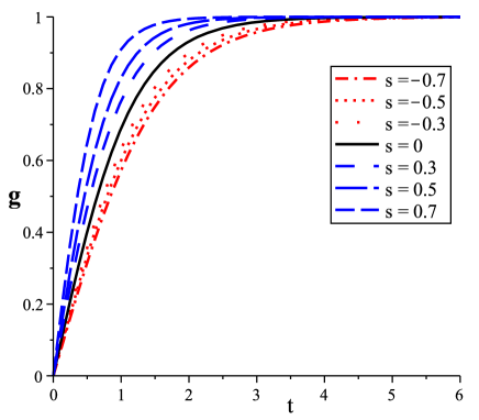
Figure 1: Scalar field $\bar{g}(t)$ (Solid black line, $s=0$, is the BPS solution for the Maxwell-Higgs model).

Figures 1 and 2 depict the numerical results obtained for the Higgs field and vector potential, showing that the profiles are drawn around the ones corresponding to the Maxwell-Higgs model. These profiles become wider for $s<0$, saturating more smoothly as $s$ becomes more negative. Otherwise, for an increasing parameter in the range $0<s<1$, the profiles continuously shrink reaching the smallest thickness for $s\rightarrow 1$.

Figure 2: Vector potential $\bar{a}(t)$.

Figure 3 depicts the magnetic field behavior. The profiles are lumps centered at the origin whose amplitudes are proportional to $(1-s)^{-1}$; hence, for $s\rightarrow 1$ higher amplitudes and narrower profiles are obtained. For $s<0$ and increasing values of $|s|$ the magnetic field profile becomes wider and wider, while its intensity continuously diminishes.

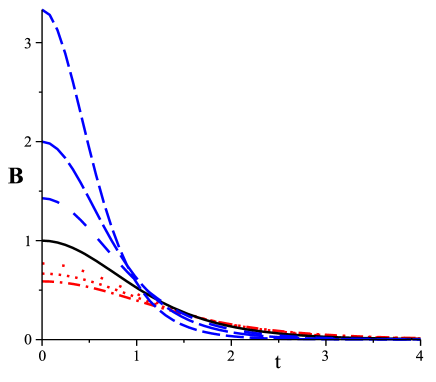
Figure 3: Magnetic field $\bar{B}(t)$.

Figure 4 shows the energy density profiles which are very similar to the magnetic field ones, but are more localized and possess greater amplitudes. This is an expected result: once the extension of the defect is reduced, its amplitude should increase in order to keep the total energy constant.

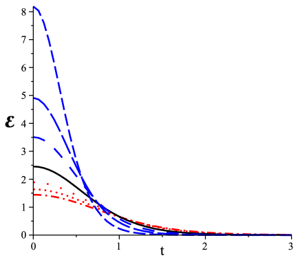
Figure 4: Energy density $\bar{\mathcal{E}}(t)$.

Both profiles belonging to the magnetic field and the energy density are useful to estimate the extension of the defect in the radial dimension. We thus note that the defect shrinks (becoming a compactlike structure) while the parameter increases inside the range $0<s<1$. It indicates that Lorentz violation works as a factor able to reduce the extension of the defect profiles. Such a reduction occurs simultaneously to the diminishment of the interaction range, revealing the consistency of this description. In the limit $s\rightarrow 1$, the theory provides a nearly null core vortex (compatible with a nearly null range).

IV Uncharged compactlike BPS vortices with fractional magnetic flux in a Lorentz-violating AMH model

In this section, we investigate uncharged vortices in a broader LV environment, keeping non-null Lorentz-violating terms in both the gauge and Higgs sectors of the Lagrangian (1). In order to restrain our study to uncharged vortices ($A_{0}=0)$ , we should require

$$\kappa_{0i}=0,\text{ }\left(k_{\phi\phi}\right)_{0i}=0,\text{ }\left(k_{\phi F}\right)_{0j}=0,$$ (40)

for which Lagrangian (1) is reduced to

$$\mathcal{L}_{1+3} =\mathcal{-}\frac{1}{4}F_{ij}F^{ij}-\frac{1}{2}\kappa^{ij}F_{i\sigma}F_{j}^{\text{ \ }\sigma}$$

$$+\left|\mathcal{D}_{i}\phi\right|^{2}+\left(k_{\phi\phi}\right)^{ij}\left(\mathcal{D}_{i}\phi\right)^{\ast}\left(\mathcal{D}_{j}\phi\right)$$ (41)

$$-\frac{1}{2}\left(k_{\phi F}\right)^{ij}F_{ij}\left|\phi\right|^{2}-U\left(\left|\phi\right|\right).$$

Under the temporal gauge the Gauss’s law is trivially solved, and Eqs. (7) and (9) are reduced to the form

$$\left(\epsilon_{jbc}-\epsilon_{jac\ }\kappa_{ab}-\kappa_{ja}\epsilon_{abc}\right)\!\partial_{b}B_{c}+\left(k_{\phi F}\right)_{ij}\partial_{j}\left[\phi^{\ast}\phi\right]$$

$$\hskip 85.35826pt=eJ_{i}-e\left(k_{\phi\phi}\right)_{ij}J_{j},$$ (42)

$$\left[\mathcal{\delta}_{ij}-\left(k_{\phi\phi}\right)_{ij}\right]\mathcal{D}_{i}\mathcal{D}_{j}\phi-\left(k_{\phi F}\right)^{ij}F_{ij}\phi-\frac{\partial U}{\partial\phi^{\ast}}=0.$$ (43)

In order to search for stable vortex configurations, we work in cylindrical coordinates $\left(r,\theta,z\right),$  implementing a modified vortex ansatz

$$\phi=\frac{v}{\Gamma^{1/2}}g\left(r\right)e^{in\theta/\Lambda},~{}\ A_{\theta}=-\frac{a\left(r\right)-n/\Lambda}{er},$$ (44)

whose form yields regular behavior for the system at $r=0$, whenever the following boundary conditions are satisfied

$$a\left(0\right)=\frac{n}{\Lambda},~{}\ \ g\left(0\right)=0.$$ (45)

In Eq. (44), in the absence of LV effects, $v$ is the vacuum expectation value of the Higgs field and $n$ the winding number of the topological solutions. The parameters $\Gamma$ and $\Lambda$ include the contributions of the Lorentz violation to the vacuum expectation of the Higgs field and the behavior of the field $a$ at the origin, respectively. As it will be shown later, the asymptotic analysis at origin of the BPS equations (49) and (51) reveals that the vortex solutions stemming from this Lorentz-violating model can only be reconciled with the modified ansatz (44). Nevertheless, the magnetic field keeps being defined as Eq.(18).

By substituting the ansatz (44) in the Ampère’s law (42), one achieves the condition

$$\left(k_{\phi\phi}\right)_{r\theta}=0,$$ (46)

and the differential equation,

$$\left(1-s\right)B^{\prime}+\frac{v^{2}}{\Gamma}\left(k_{\phi F}\right)_{r\theta}\left(g^{2}\right)^{\prime}+2e\frac{v^{2}}{\Gamma}\frac{ag^{2}}{r}\left[1-\left(k_{\phi\phi}\right)_{\theta\theta}\right]=0,$$ (47)

where $s=\kappa_{rr}+\kappa_{\theta\theta}$.

The Higgs equation of motion (43) now is

$$\left[1-\left(k_{\phi\phi}\right)_{rr}\right]\left(g^{\prime\prime}+\frac{g^{\prime}}{r}\right)-\left[1-\left(k_{\phi\phi}\right)_{\theta\theta}\right]\frac{a^{2}}{r^{2}}g$$

$$\hskip 56.9055pt+\left(k_{\phi F}\right)_{r\theta}Bg+\frac{\Gamma}{2v^{2}}\frac{\partial U}{\partial g}=0.$$

This equation can only be written as a first-order differential equation if we assume a generalized self-duality condition, that is,

$$g^{\prime}=\pm\Lambda\frac{ag}{r},$$ (49)

with the parameter $\Lambda$ conveniently defined as

$$\Lambda=\sqrt{\frac{1-\left(k_{\phi\phi}\right)_{\theta\theta}}{1-\left(k_{\phi\phi}\right)_{rr}}}.$$ (50)

The BPS equation (49) also allows us to integrate the Ampère’s law (47), yielding another first-order equation involving $a^{\prime}$

$$-\frac{a^{\prime}}{er}=B=\pm\frac{ev^{2}}{1-s}\left(1-g^{2}\right),$$ (51)

which is the second BPS equation. It is exactly the same one obtained in the previous section (see Eq. (24)). Then, by using the BPS equations in (LABEL:NHiggs3a) it is possible to compute the BPS fourth-order self-interacting potential,

$$U\left(g\right)=\frac{e^{2}v^{4}}{2\left(1-s\right)}\left(1-g^{2}\right)^{2},$$ (52)

that written in terms of the Higgs field gives

$$U\left(\left|\phi\right|\right)=\frac{\Gamma^{2}e^{2}}{2\left(1-s\right)}\left(\frac{v^{2}}{\Gamma}-\left|\phi\right|^{2}\right)^{2},$$ (53)

with

$$\Gamma =\eta\pm\frac{\left(k_{\phi F}\right)_{r\theta}}{e},$$ (54)

$$\eta =\sqrt{\left[1-\left(k_{\phi\phi}\right)_{\theta\theta}\right]\left[1-\left(k_{\phi\phi}\right)_{rr}\right]}.$$ (55)

It reveals that this theory may support two different vacua,

$$\left|\phi\right|=\frac{v}{\sqrt{\eta\pm\displaystyle\frac{\left(k_{\phi F}\right)_{r\theta}}{e}}},$$ (56)

induced by the coefficient $\left(k_{\phi F}\right)_{r\theta}.$ We point out that for each vacuum in (56) there exists topological defect solutions of definite vorticity, once the $\left(+\right)$ vacuum supports defects having only a positive winding number $\left(n>0\right)$ whereas the $\left(-\right)$ vacuum is related to vortices with negative winding number $\left(n<0\right)$. It is known that the Maxwell-Higgs solutions present the following correspondence: the ones represented with $a\left(r\right)$ and $g\left(r\right)$ for $n>0$ are mapped in solutions with $n<0$ by doing $a\left(r\right)\rightarrow-a\left(r\right)$ and $g\left(r\right)\rightarrow g\left(r\right)$. This correspondence is broken in a theory endowed with the vacuum (56), which could be associated with the breaking of the discrete symmetry connecting the solutions with $n>0$ and $n<0$. The physical soundness of this hypothesis is still to be verified after analysis concerning energy stability.

Now, adopting the conditions (40) and setting the temporal gauge $\left(A_{0}=0\right)$, we evaluate the energy density for this stationary and uncharged system as

$$\mathcal{E} =\frac{1}{2}\left(1-\kappa_{jj}\right)B^{2}+\left|\mathcal{D}_{j}\phi\right|^{2}-\left(k_{\phi\phi}\right)_{ij}\left(\mathcal{D}_{i}\phi\right)^{\ast}\left(\mathcal{D}_{j}\phi\right)$$

$$\quad+\left(k_{\phi F}\right)_{12}B\left|\phi\right|^{2}+U\left(\left|\phi\right|\right).$$ (57)

After replacing the ansatz (44) and implementing the BPS procedure, it is rewritten as

$$\mathcal{E} =\frac{1}{2}\left(1-s\right)\left[B\mp\frac{ev^{2}}{1-s}\left(1-g^{2}\right)\right]^{2}$$

$$\quad+\frac{v^{2}}{\Gamma}\left[1-\left(k_{\phi\phi}\right)_{rr}\right]\left[\!\frac{{}}{{}}g^{\prime}\mp\Lambda\frac{ag}{r}\right]^{2}$$ (58)

$$\quad\pm Bev^{2}\mp e\frac{v^{2}}{\Gamma}\eta Bg^{2}\pm 2\frac{v^{2}}{\Gamma}\eta\frac{ag}{r}g^{\prime}.$$

Requiring energy minimization, the squared brackets must vanish, yielding the BPS equations (51) and (49), respectively.

Imposing the BPS conditions in Eq. (58), one achieves the BPS energy density which is simplified to the form

$$\mathcal{E}_{BPS}=\mp v^{2}\frac{a^{\prime}}{r}\pm\eta\frac{v^{2}}{\Gamma}\frac{\left(ag^{2}\right)^{\prime}}{r},$$ (59)

whose integration, considering the following asymptotic conditions,

$$a\left(\infty\right)=0,~{}\ \ g\left(\infty\right)=1,$$ (60)

leads to the total BPS energy

$$E_{BPS}=\frac{v^{2}}{\Lambda}\left|n\right|.$$ (61)

So, we must notice that the total BPS energy is not affected by the difference between the two vacua (56), associated, in principle, with the spontaneous breaking of some discrete symmetry.

It is very interesting to note that magnetic flux is now a multiple of the fractional ratio $2\pi/e\Lambda,$ that is,

$$\Phi_{B}=\int B\left(r\right)d^{2}\mathbf{r}=\frac{2\pi}{e\Lambda}n,$$ (62)

indicating that this model provides fractional vortex solutions, which have been recently reported in condensed matter literature PRL . Note that the relation between the total energy and magnetic flux, $H_{\min}=ev^{2}\left|\Phi_{B}\right|,$ continues to be valid.

By using the BPS equations, the energy density (59) can be written as

$$\mathcal{E}_{BPS}=\frac{e^{2}v^{4}\eta}{\left(1-s\right)\Gamma}\left(\frac{\Gamma}{\eta}-g^{2}\right)\left(1-g^{2}\right)+2v^{2}\frac{\eta\Lambda}{\Gamma}\left(\frac{ag}{r}\right)^{2},$$ (63)

which is not a positive-definite expression. The energy density (57) shows explicitly that the parameter $\left(k_{\phi F}\right)_{r\theta}$ is responsible for this energy instability. Hence, one must require $\left(k_{\phi F}\right)_{r\theta}=0$ for assuring energy stability. Under such condition we have $\Gamma=\eta$, and Eq. (63) provides a positive-definite BPS energy density

$$\mathcal{E}_{BPS}=\left(1-s\right)B^{2}+2v^{2}\Lambda\left(\frac{ag}{r}\right)^{2},$$ (64)

whenever $s<1$ and $\left(k_{\phi\phi}\right)_{rr},\left(k_{\phi F}\right)_{\theta\theta}<1$.  Similarly, with $\left(k_{\phi F}\right)_{r\theta}=0$, the truly BPS self-interacting potential becomes

$$U=\frac{e^{2}\eta^{2}}{2\left(1-s\right)}\left(\frac{v^{2}}{\eta}-\left|\phi\right|^{2}\right)^{2},$$ (65)

providing a unique modified vacuum,

$$\left|\phi\right|\mathbf{=}\frac{v}{\sqrt{\eta}}\mathbf{,}$$ (66)

that supports solutions with two vorticities, as is usual. So, we highlight that the consistent uncharged vortex solutions of this model are the ones ruled by Eqs. (49) and (51), with self-interacting potential (65), and the modified vacuum expectation value (66). Note that the LV Higgs coefficients modify the usual self-duality condition (23) and the vacuum of the Maxwell-Higgs model.

One should still discuss the reason that requires the modified vortex ansatz (44). First, note that if we had supposed the usual ansatz (16), one would have achieved the same BPS equations given by (49) and (51). On the other hand, performing the series expansion at $r=0$ of the regular functions $g\left(r\right),a\left(r\right)$ fulfilling the BPS equations, we obtain

$$g\left(r\right) =Gr^{\left|n\right|}-\frac{\Lambda G\left(ev\right)^{2}}{4\left(1-s\right)}r^{\left|n\right|+2}+\mathcal{\ldots},$$ (67)

$$a\left(r\right) =\frac{n}{\Lambda}-\frac{\left(evr\right)^{2}}{2\left(1-s\right)}+\frac{\left(Gev\right)^{2}~{}r^{2\left|n\right|+2}}{2\left(1-s\right)\left(\left|n\right|+1\right)}+\mathcal{\ldots},$$ (68)

where $G$ is a constant. It is easy to notice that the expansion (68) is incompatible with the usual ansatz (16), stating an inconsistency. In order to avoid it we have adopted the new ansatz (44), keeping the field $A_{\theta}$ finite at $r=0.$

We now present the asymptotic behavior at $r=\infty$. By setting

$$g\left(r\right)=1+\delta g,~{}\ \ \ a\left(r\right)=\delta a,$$ (69)

and after solving the linearized BPS equations for $\delta g$ and $\delta a$, we obtain

$$\delta g =-\frac{G_{1}}{ev}\sqrt{\frac{\Lambda\left(1-s\right)}{2}}K_{0}\left(rev\sqrt{\frac{2\Lambda}{1-s}}\right),~{}\ \$$ (70)

$$\delta a =G_{1}~{}r~{}K_{1}\left(rev\sqrt{\frac{2\Lambda}{1-s}}\right),$$ (71)

from which we observe that the mass of the gauge and Higgs fields is

$$m_{A}=m_{H}=ev\sqrt{\frac{2\Lambda}{1-s}}.$$ (72)

In this case, notice that there are two LV parameters modifying the mass. For a fixed $\Lambda$, it holds the behavior described after Eq. (39) for compactlike defects. For a fixed $s,$ we observe that the mass increases with $\Lambda$, in opposition to its dependence with $s.$

In order to facilitate the numerical analysis of the vortex profiles, we first introduce the dimensionless variable, $t=ev\Lambda^{1/2}r,$ and the following field redefinitions:

$$g\left(r\right)\rightarrow\bar{g}\left(t\right),~{}\ \ a\left(r\right)\rightarrow\frac{\bar{a}\left(t\right)}{\Lambda};$$ (73)

with the new variable, the BPS equations (49) and (51) are rewritten as

$$\bar{g}^{\prime}=\pm\frac{\bar{a}\bar{g}}{t},\text{ \ \ }-\frac{\bar{a}^{\prime}}{t}=\bar{B}=\pm\frac{1-\bar{g}^{2}}{\left(1-s\right)},$$ (74)

assuming the same form as Eqs. (31) and (32). This shows that under the conditions that provide uncharged vortex configurations the broader model of Lagrangian (1) also supports compactlike solutions with controllable size as well.

However, note that the field rescaling (73) into the full Lagrangian (1) does not yield the model of Lagrangian (10) at all.  It is important to note that a simple field rescaling in the Lagrangian (10) does not lead to the fractional vortices engendered by Lagrangian (1). In this sense, note that the rescaling$\ \bar{a}\rightarrow\bar{a}/\Lambda$ whenever applied into Eq. (35) leads to

$$\bar{a}\left(t\right)=\frac{n}{\Lambda}-\frac{\ t^{2}}{2\left(1-s\right)\Lambda}+\frac{G^{2}~{}t^{2\left|n\right|+2}}{2\left(1-s\right)(\left|n\right|+1)\Lambda}+\mathcal{\ldots}.$$ (75)

This equation is consistent with the ansatz (44), indicating fractional magnetic flux. Nevertheless, it does not represent the original magnetic field for the uncharged vortex stemming from Lagrangian (10). Indeed, while this series leads to $B(0)=\left[\left(1-s\right)\Lambda\right]^{-1}$, the correct result is the one of Eq. (33). This means that the physical equivalence between the models belonging to the Lagrangians (1) and (10) could be established by performing adequate coordinates and field transformations, as discussed below using polar coordinates and by means of a general coordinate system in the Appendix.

Once the BPS equations are equal, and the asymptotic conditions are qualitatively similar, one asserts that the vortex profiles stemming from Eqs. (49) and (51) present the same behavior of the ones depicted in Figs. 1, 2, 3, 4. In this way, a numerical evaluation of the new corresponding profiles becomes unnecessary.

There exist some maps connecting the models of Lagrangians (1) and (10). For example, in polar coordinates such mapping is easily observed: it involves a simultaneous rescaling of the radial coordinate and the gauge field. By writing the energy density (57) with $\left(k_{\phi F}\right)_{12}=0$ in polar coordinates, we have

$$E =2\pi{\displaystyle\int}dr~{}r\left[\frac{1}{2}\left(1-s\right)B^{2}+\frac{v^{2}}{\Lambda}\left(g^{\prime}\right)^{2}+v^{2}\Lambda\frac{\left(ag\right)^{2}}{r^{2}}\right.$$ (76)

$$~{}\ \ \ \ \ \left.~{}\ \ \ \ \ \ \ \ \ \ \ \ +\frac{v^{4}e^{2}}{2\left(1-s\right)}\left(1-g^{2}\right)^{2}\right].$$

Performing the rescaling,

$$r=\frac{\bar{r}}{\Lambda^{1/2}},\ \ a\left(r\right)\rightarrow\frac{a\left(\bar{r}\right)}{\Lambda},~{}\ \ g\left(r\right)\rightarrow g\left(\bar{r}\right),~{}$$ (77)

we obtain

$$E =\frac{2\pi}{\Lambda}{\displaystyle\int}d\bar{r}~{}\bar{r}\left\{\frac{1}{2}\left(1-s\right)\left(\frac{a^{\prime}}{e\bar{r}}\right)^{2}+v^{2}\left[\left(g^{\prime}\right)^{2}+\frac{\left(ag\right)^{2}}{\bar{r}^{2}}\right]\right.$$

$$~{}\ \ \ \ \left.\ ~{}\ \ \ \ \ \ \ \ \ \ \ \ +\frac{v^{4}e^{2}}{2\left(1-s\right)}\left(1-g^{2}\right)^{2}\right\}.$$ (78)

The term in bracket is the energy density (15), expressed in polar coordinates, for the vortices of the simpler model studied in Sec. III. In Cartesian coordinates this mapping would be more involved, including a rotation followed by a coordinate rescaling in order to transform the Higgs sector of the Lagrangian (1) into the one of (10). Obviously, such transformations would also affect the gauge sector by adding LV Higgs contributions to the already existent LV gauge parameters. At this point, it would still be necessary to perform a gauge field rescaling in order to transform completely (1) into (10). This set of transformations is easily performed in polar coordinates, as shown in (77).

V Conclusions

In this work, we have investigated the existence of stable uncharged BPS vortex configurations in the framework of an Abelian Maxwell-Higgs model supplemented with CPT-even and Lorentz-violating terms belonging to the gauge and Higgs sectors of the standard model extension. Our study has accounted two situations: the first one considered LV terms only in the gauge sector while the second case regarded the full model. In both cases we have restrained the investigation to uncharged topological solutions. In the first case, we have found the equations of motion and implemented the usual ansatz for static and rotationally symmetric vortex solutions. By applying the Bogomol’nyi method to the energy density, the first-order BPS equations were achieved, exhibiting a similar structure to the ones of the Abelian Maxwell-Higgs model which supports the ANO vortices. A numerical procedure was used to unveil the profiles of the BPS vortex solutions. Although the governing equations present the same structure, the LIV parameter, $s$, appears as a key element that allows us to control the thickness (radial extent) of the defect while spanning the available range $\left(s<1\right)$: the larger is the value of the LIV parameter, $s$; the narrower is the profile of the vortex, and vice versa. The intensity of the magnetic field increases with $s$, tending to a maximal value when $s\rightarrow 1,$ a limit in which the length of the defect and the interaction range tends to zero. Our results offer the possibility of controlling the extension of the defect without modifying the kinetic sector or the Higgs potential of the model. In this theoretical framework, Lorentz violation (for $0<s<1$) plays a role similar to some nonlinear kinetic terms usual in k-field theories, which yield compactlike defects Hora1 ; Compact1 ; kfield ; Hora2 ; Hora3 . Despite the profile shrinking observed here, analogous to the one verified in k-field compactlike defects (see Ref. Hora2 ), one should point out some advantages of the Lorentz-violating compactlike solutions: the BPS character, the preservation of the usual kinetic sector of the Maxwell-Higgs theory, and the direct correspondence between the defect thickness and the range of the interaction. Moreover, this result opens a new window: the chance of employing models with Lorentz violation as an effective theory to address some situations wherein k-field models have been applied (see Refs.Cosmology ; DM ; Tachyon ; GC ; kfield ), with special attention to topological defects. More specifically, the possibility of controlling the interaction range and the size of the defect may allow interesting applications to the investigation of vortex configurations in some condensed matter frameworks, where the penetration length depends on the properties of system.

One should remark that the vortex solutions provided by Eqs. (23) and (24) do not exhibit space anisotropy, although the LV parity-even coefficients usually yield anisotropic stationary solutions (see Ref.Paulo1 ). This indicates that the vortex ansatz selects only the parity-even solutions not endowed with space anisotropy. We still remember that the vortex configurations obtained in this Lorentz-violating model are somehow equivalent to the ones yielded by the effective Maxwell-Higgs electrodynamics of Ref. Dielectric , which describes vortex configurations in a continuum medium. Note that in this situation it does not make sense to consider vacuum upper bounds on the Lorentz-violating coefficients, once the role of the Lorentz-violating coefficient is to state the presence of the dielectric medium. This interpretation turns sensible the profile analysis performed in this work for the range $-1<s<1$, which obviously involves magnitudes much higher than the upper bounds usually stated, for example, in an electrodynamics in the vacuum.

Lastly, we have addressed the case where the Lorentz violation is present in the Higgs and gauge sectors simultaneously. The equations of motion were determined, being possibly compatible with BPS equations defined in the context of a theory with two different vacua, each one supporting a definite vorticity solution. The energy density was carried out, revealing that only one of the Higgs LV coefficients yields solutions with energy stability, so that we have adopted $\left(k_{\phi F}\right)_{r\theta}=0.$ The remaining theory provides stable uncharged vortices (with both vorticities) in a unique vacuum. It has implied BPS equations consisting of a modified duality relation and compatible with a new rotationally symmetric vortex ansatz. After an appropriated coordinate and field rescaling, such equations recover the BPS equations of the first case (with Lorentz violation only in the gauge sector), leading to vortex solutions with similar profiles but different magnetic flux. In this case, however, the defect profiles are controlled by two LV parameters, $\Lambda$ and $s,$ that play opposite roles on the spatial extension and the range of the interaction. For a fixed $\Lambda,$ we recover the same phenomenology described for the first case. For a fixed $s,$ the size of the vortex should diminish with an increasing $\Lambda.$ Hence, we notice that $\Lambda$ and $s$ act as competing parameters, providing a larger control on the solution.  The crucial difference between the first and the second model is entailed with the new vortex ansatz required to imply consistent solutions at origin. Such difference engenders an interesting novelty: vortices with fractional magnetic flux, which is a feature of interest in condensed matter systems, as, for example, in recent models for superconductivity PRL where the vortex solutions have a fractional structure. Finally, we highlight that the fractional BPS solutions are explicitly defined in the context of a modified vacuum theory, in accordance with Eq.(66). The point is that in the presence of the LV-Higgs parameters, the self-interacting fourth-order potential must be given as in Eq. (65) for ensuring the existence of BPS solutions.  In the Appendix, we discuss the equivalence between the models of Lagrangians (1) and (10). Such an equivalence leads to the conclusion that the simpler model of Lagrangian (10) should also possess fractional solutions, in principle uncovered, and only revealed by suitable coordinate transformations.

New developments in this Lorentz-violating environment are now under way, mainly in connection with the search for charged vortex configurations, in the absence of the Chern-Simons term, when the Higgs sector is supplemented with a richer self-interacting potential Carlisson2 . Finally, an interesting investigation would be to verify the existence of topological defects in the non-Abelian sector of the SME.

VI Appendix

In this Appendix we comment on the existence of a coordinate transformation stating the equivalence of the models of Lagrangians (1) and (10) at first order in the Lorentz-violating parameters. This coordinate transformation can be generally written as

$$x^{\mu} =\left(M^{-1}\right)^{\mu}{}_{\nu}x^{\prime\nu},~{}\ \ \partial_{\mu}=M^{\nu}{}_{\mu}\partial_{\nu}^{\prime},$$

$$A_{\mu} =M^{\nu}{}_{\mu}A_{\nu}^{\prime},~{}\ \mathcal{D}_{\mu}\phi=M^{\nu}{}_{\mu}\mathcal{D}_{\nu}^{\prime}\phi.$$

We can show that this transformation yields

$$\mathcal{L}_{\phi} =\left|\mathcal{D}_{\mu}\phi\right|^{2}+\left(k_{\phi\phi}\right)^{\mu\nu}\left(\mathcal{D}_{\mu}\phi\right)^{\ast}\left(\mathcal{D}_{\nu}\phi\right)$$

$$=\left[g^{\mu\nu}+\left(k_{\phi\phi}\right)^{\mu\nu}\right]\left(\mathcal{D}_{\mu}\phi\right)^{\ast}\left(\mathcal{D}_{\nu}\phi\right)$$

$$=g^{\prime\alpha\beta}\left(\mathcal{D}_{\alpha}^{\prime}\phi\right)^{\ast}\left(\mathcal{D}_{\beta}^{\prime}\phi\right),$$ (80)

where $g^{\prime\alpha\beta}$ is a new metric tensor related to $g^{\mu\nu}$ via the equation

$$\left[g^{\mu\nu}+\left(k_{\phi\phi}\right)^{\mu\nu}\right]M^{\alpha}{}_{\mu}M^{\beta}{}_{\nu}=g^{\prime\alpha\beta}.$$ (81)

At the first order, $M^{\alpha}{}_{\mu}$ can be written as

$$M^{\alpha}{}_{\mu}=\delta^{\alpha}{}_{\mu}+m^{\alpha}{}_{\mu},$$ (82)

which, when replaced in Eq.(81) leads to

$$g^{\alpha\beta}+m^{\beta\alpha}+m^{\alpha\beta}+\left(k_{\phi\phi}\right)^{\alpha\beta}=g^{\prime\alpha\beta}.$$ (83)

At this point, we can organize the possible maps into two possibilities.

VI.1 First case

A preliminary case is addressed when one requires

$$m^{\beta\alpha}=m^{\alpha\beta}=-\frac{1}{2}\left(k_{\phi\phi}\right)^{\alpha\beta},$$ (84)

so that Eq. (82) reads as

$$M^{\alpha}{}_{\mu}=\delta^{\alpha}{}_{\mu}-\frac{1}{2}\left(k_{\phi\phi}\right)^{\alpha}{}_{\mu},$$ (85)

and the metric remains unaffected, $g^{\alpha\beta}=g^{\prime\alpha\beta}.$ Within this context, one explicitly evaluates

$$\mathcal{L}_{F} =\mathcal{-}\frac{1}{4}F_{\mu\nu}F^{\mu\nu}-\frac{1}{2}\kappa^{\rho\alpha}F_{\rho\sigma}F_{\alpha}^{\text{ \ }\sigma}$$

$$=\mathcal{-}\frac{1}{4}F_{\alpha\beta}^{\prime}F^{\prime\alpha\beta}-\frac{1}{2}\kappa^{\prime\alpha\delta}F_{\alpha\beta}^{\prime}F_{\delta}^{\prime}~{}^{\beta},$$ (86)

where we have defined

$$\kappa^{\prime\alpha\delta}=\kappa^{\alpha\delta}-\left(k_{\phi\phi}\right)^{\alpha\delta}.$$ (87)

Therefore, under the coordinate transformation (85), and at first order in the LV parameters, the full Lagrangian,

$$\mathcal{L} =\mathcal{-}\frac{1}{4}F_{\mu\nu}F^{\mu\nu}-\frac{1}{2}\kappa^{\rho\alpha}F_{\rho\sigma}F_{\alpha}^{\text{ \ }\sigma}+\left|\mathcal{D}_{\mu}\phi\right|^{2}$$ (88)

$$+\left(k_{\phi\phi}\right)^{\mu\nu}\left(\mathcal{D}_{\mu}\phi\right)^{\ast}\left(\mathcal{D}_{\nu}\phi\right)-U\left(\left|\phi\right|\right),$$

becomes equivalent to

$$\mathcal{L}=\mathcal{-}\frac{1}{4}F_{\mu\nu}^{\prime}F^{\prime\mu\nu}-\frac{1}{2}\kappa^{\prime\rho\alpha}F_{\rho\sigma}^{\prime}F_{\alpha}^{\prime\text{ \ }\sigma}+\left|\mathcal{D}_{\mu}^{\prime}\phi\right|^{2}-U\left(\left|\phi\right|\right),$$ (89)

revealing that the Lorentz-violating terms were moved from the scalar to the gauge sector.

VI.2 Second case

Another possibility consists in taking

$$m^{\alpha\beta}=-m^{\beta\alpha},$$ (90)

so that $M^{\alpha}{}_{\mu}$ is an orthogonal matrix at first order. The metric relation (83) is now

$$g^{\prime\alpha\beta}=g^{\alpha\beta}+\left(k_{\phi\phi}\right)^{\alpha\beta},$$ (91)

representing a nondiagonal matrix. At first order,

$$M^{\alpha}{}_{\mu}M^{\beta}{}_{\nu} =\delta^{\alpha}{}_{\mu}\delta^{\beta}{}_{\nu}+\delta^{\alpha}{}_{\mu}m^{\beta}{}_{\nu}+m^{\alpha}{}_{\mu}\delta^{\beta}{}_{\nu},$$

(92)

$$g^{\mu\nu}M^{\alpha}{}_{\mu}M^{\beta}{}_{\nu} =g^{\alpha\beta}~{},~{}\left(k_{\phi\phi}\right)^{\mu\nu}M^{\alpha}{}_{\mu}M^{\beta}{}_{\nu}=\left(k_{\phi\phi}\right)^{\alpha\beta}.$$

Using the first-order relations (92), after some algebra we can explicitly show that

$$\mathcal{L}_{F} =\mathcal{-}\frac{1}{4}F_{\mu\nu}F^{\mu\nu}-\frac{1}{2}\kappa^{\rho\alpha}F_{\rho\sigma}F_{\alpha}^{\text{ \ }\sigma}$$

$$=\mathcal{-}\frac{1}{4}F_{\mu\nu}^{\prime}F^{\prime\mu\nu}-\frac{1}{2}\kappa^{\prime\rho\alpha}F_{\rho\sigma}^{\prime}F_{\alpha}^{\prime\text{ \ }\sigma},$$ (93)

with the redefinition (87). Therefore, at first order in LIV parameters, under the coordinate transformation (VI), the full Lagrangian (88) becomes

$$\mathcal{L}^{\prime} =\mathcal{-}\frac{1}{4}F_{\mu\nu}^{\prime}F^{\prime\mu\nu}-\frac{1}{2}\kappa^{\prime\rho\alpha}F_{\rho\sigma}^{\prime}F_{\alpha}^{\prime}{}^{\sigma}$$

$$+g^{\prime\mu\nu}\left(\mathcal{D}_{\mu}^{\prime}\phi\right)^{\ast}\left(\mathcal{D}_{\nu}^{\prime}\phi\right)-U\left(\left|\phi\right|\right),$$ (94)

with the observation that the metric $g^{\prime\mu\alpha}$ is nondiagonal. It can be achieved as a set of transformations (at first order) turning $g^{\prime\mu\nu}$ diagonal, and stating the equivalence of the models of Lagrangians (88) and (94).

We have thus stated the equivalence between the models (88) and (89) at first order in the Lorentz-violating parameters. Notwithstanding, a more involved transformation may be found assuring the full equivalence at any order. This fact is related to physical observability of the LV parameters in the scalar and gauge sectors of the model. For a more complete discussion about this point, see Sec. II, part C, of Ref. Gravity2 . The physical equivalence of the models of Lagrangians (1) and (10) [with $\left(k_{\phi F}\right)^{\mu\nu}=0$] leads to the conclusion that the fractional vortex configurations are explicit solutions of the model of Lagrangian (1) and hidden solutions of the Lagrangian (10).

- (1) A. Abrikosov, Sov. Phys. JETP 32, 1442 (1957); H. Nielsen and P. Olesen, Nucl. Phys.B61, 45 (1973).
- (2) S. Deser, R. Jackiw, and S. Templeton, Ann. Phys. (NY) 140, 372 (1982); G.V. Dunne, arXiv:hep-th/9902115.
- (3) R. Jackiw and E. J. Weinberg, Phys. Rev. Lett. 64, 2234 (1990); R. Jackiw, K. Lee, and E.J. Weinberg, Phys. Rev. D42, 3488 (1990); J. Hong, Y. Kim, and P.Y. Pac, Phys. Rev. Lett. 64, 2230 (1990); G.V. Dunne, Self-Dual Chern-Simons Theories (Springer, Heidelberg, 1995).
- (4) Z.F. Ezawa, Quantum Hall Effects, ( World Scientific, 2000 ).
- (5) P.K. Ghosh, Phys. Rev. D 49, 5458 (1994); T. Lee and H. Min, Phys. Rev. D 50, 7738 (1994).
- (6) N. Sakai and D. Tong, J. High Energy Phys. 03, 019 (2005); G. S. Lozano, D. Marques, E. F. Moreno, and F. A. Schaposnik, Phys. Lett. B 654, 27 (2007).
- (7) S. Bolognesi and S.B. Gudnason, Nucl. Phys. B805, 104 (2008).
- (8) D. Bazeia, E. da Hora, C. dos Santos, and R. Menezes, Phys. Rev. D 81, 125014 (2010).
- (9) C. dos Santos, Phys. Rev. D 82, 125009 (2010).
- (10) D. Bazeia, E. da Hora, C. dos Santos, and R. Menezes, Eur. Phys. J. C 71, 1833 (2011).
- (11) D. Bazeia, E. da Hora, and R. Menezes, Phys. Rev. D 85, 045005 (2012).
- (12) C. Armendariz-Picon, T. Damour, and V. Mukhanov, Phys. Lett. B 458, 209 (1999).
- (13) C. Armendariz-Picon and E. A. Lim, J. Cosmol. Astropart. Phys. 08, 007 (2005).
- (14) A. Sen, J.High Energy Phys. 07, 065 (2002).
- (15) N. Arkani-Hamed, H.-C. Cheng, M. A. Luty, and S. Mukohyama, J.High Energy Phys. 05, 074 (2004); N. Arkani-Hamed, P. Creminelli, S. Mukohyama, and M. Zaldarriaga, J. Cosmol. Astropart. Phys. 04, 001 (2004); S. Dubovsky, J. Cosmol. Astropart. Phys. 07, 009 (2004); D. Krotov, C. Rebbi, V. Rubakov, and V. Zakharov, Phys.Rev. D 71, 045014 (2005); A. Anisimov and A. Vikman, J. Cosmol. Astropart. Phys. 04, 009 (2005).
- (16) E. Babichev, Phys. Rev. D 74, 085004 (2006); Phys. Rev. D 77, 065021 (2008).
- (17) D. Bazeia, E. da Hora, R. Menezes, H. P. de Oliveira, and C. dos Santos, Phys. Rev. D 81, 125016 (2010).
- (18) C. dos Santos and E. da Hora, Eur. Phys. J. C 70, 1145 (2010); Eur. Phys. J. C 71, 1519 (2011); D. Bazeia, E. da Hora, D. Rubiera-Garcia, Phys. Rev. D 84, 125005 (2011).
- (19) P. Rosenau and J.M. Hyman, Phys. Rev. Lett. 70, 564 (1993); P. Rosenau and E. Kashdan, Phys. Rev. Lett. 104, 034101(2010).
- (20) C. Adam, P. Klimas, J. Sánchez-Guillén, and A. Wereszczyński, J. Math. Phys. 50, 102303 (2009); C. Adam, N. Grandi, J. Sanchez-Guillen and A. Wereszczynski, J. Phys. A 41, 212004 (2008); C. Adam, P Klimas, J Sánchez-Guillén and A. Wereszczynski, J. Phys. A 42, 135401 (2009).
- (21) D. Colladay and V. A. Kostelecky, Phys. Rev. D 55, 6760 (1997); D. Colladay and V. A. Kostelecky, Phys. Rev. D 58, 116002 (1998); S. R. Coleman and S. L. Glashow, Phys. Rev. D 59, 116008 (1999); S.R. Coleman and S.L. Glashow, Phys. Rev. D 59, 116008 (1999).
- (22) V. A. Kostelecky and S. Samuel, Phys. Rev. Lett. 63, 224 (1989); Phys. Rev. Lett. 66, 1811 (1991); Phys. Rev. D 39, 683 (1989); Phys. Rev. D 40, 1886 (1989); V. A. Kostelecky and R. Potting, Nucl. Phys. B 359, 545 (1991); Phys. Lett. B381, 89 (1996); V. A. Kostelecky and R. Potting, Phys. Rev. D 51, 3923 (1995).
- (23) B. Altschul, Phys. Rev. D 70, 056005 (2004); G. M. Shore, Nucl. Phys. B717, 86 (2005); D. Colladay and V. A. Kostelecky, Phys. Lett. B 511, 209 (2001); O. G. Kharlanov and V. Ch. Zhukovsky, J. Math. Phys. 48, 092302 (2007); R. Lehnert, Phys. Rev. D 68, 085003 (2003); V.A. Kostelecky and C. D. Lane, J. Math. Phys. 40, 6245 (1999); R. Lehnert, J. Math. Phys. 45, 3399 (2004); V. A. Kostelecky and R. Lehnert, Phys. Rev. D 63 , 065008 (2001); W. F. Chen and G. Kunstatter, Phys. Rev. D 62, 105029 (2000); B. Goncalves, Y. N. Obukhov, and I. L. Shapiro, Phys.Rev.D 80, 125034 (2009).
- (24) M. Gomes, J. R. Nascimento, A. Yu. Petrov, and A. J. da Silva, Phys. Rev. D 81, 045018 (2010); T. Mariz, J. R. Nascimento, A. Yu. Petrov, Phys. Rev. D 85, 125003 (2012); T. Mariz, J. R. Nascimento, and A.Yu. Petrov, Phys. Rev. D 85, 125003 (2012); G. Gazzola, H. G. Fargnoli, A. P. Baeta Scarpelli, M. Sampaio, and M. C. Nemes, J. Phys. G 39, 035002 (2012); A. P. Baeta Scarpelli, Marcos Sampaio, M. C. Nemes, and B. Hiller, Eur. Phys. J. C 56, 571 (2008); F.A. Brito, L.S. Grigorio, M.S. Guimaraes, E. Passos, and C. Wotzasek, Phys.Rev. D 78, 125023 (2008); F.A.Brito, E. Passos, and P.V. Santos, Europhys. Lett. 95, 51001 (2011).
- (25) K. Bakke and H. Belich, J. Phys. G 39,085001 (2012); K. Bakke, H. Belich, and E. O. Silva, J. Math. Phys. 52, 063505 (2011); J. Phys. G 39, 055004 (2012); Ann. Physik (Leipzig) 523, 910 (2011).
- (26) V. A. Kostelecky, Phys. Rev. D 69, 105009 (2004); V. A. Kostelecky, N. Russell, and J. D. Tasson, Phys. Rev. Lett. 100, 111102 (2008); V. A. Kostelecky and J. D. Tasson, Phys. Rev. Lett. 102, 010402 (2009); Q. G. Bailey and V.A. Kostelecky, Phys.Rev. D 74, 045001 (2006); Q. G. Bailey, Phys.Rev. D 80, 044004 (2009); V.A. Kostelecky and R. Potting, Phys.Rev. D 79, 065018 (2009); Q. G. Bailey, Phys. Rev. D 82, 065012 (2010); V.B. Bezerra, C.N. Ferreira and J.A. Helayel-Neto, Phys.Rev. D 71, 044018 (2005); J.L. Boldo, J.A. Helayel-Neto, L.M. de Moraes, C.A.G. Sasaki and V.J. V. Otoya, Phys. Lett. B 689, 112 (2010).
- (27) V. A. Kostelecky and J. D. Tasson, Phys. Rev. D 83, 016013 (2011).
- (28) S.M. Carroll, G.B. Field, and R. Jackiw, Phys. Rev. D 41, 1231 (1990).
- (29) V. A. Kostelecky and M. Mewes, Phys. Rev. Lett. 87, 251304 (2001).
- (30) V. A. Kostelecky and M. Mewes, Phys. Rev. D 66, 056005 (2002); V. A. Kostelecky and M. Mewes, Phys. Rev. Lett. 97, 140401 (2006).
- (31) B. Altschul, Nucl. Phys. B796, 262 (2008); B. Altschul, Phys. Rev. Lett. 98, 041603 (2007); C. Kaufhold and F.R. Klinkhamer, Phys. Rev. D 76, 025024 (2007).
- (32) F.R. Klinkhamer and M. Risse, Phys. Rev. D 77, 016002 (2008); F.R. Klinkhamer and M. Risse, Phys. Rev. D 77, 117901 (2008).
- (33) F. R. Klinkhamer and M. Schreck, Phys. Rev. D 78, 085026 (2008).
- (34) Q. Exirifard, Phys. Lett. B 699, 1 (2011).
- (35) V. A. Kostelecky and M. Mewes, Phys. Rev. D 80, 015020 (2009); M. Cambiaso, R. Lehnert, and R. Potting, Phys.Rev. D 85 085023 (2012); M. Mewes, Phys. Rev. D 85, 116012 (2012).
- (36) M.N. Barreto, D. Bazeia, and R. Menezes, Phys.Rev. D73, 065015 (2006); A. de Souza Dutra, M. Hott, and F. A. Barone, Phys. Rev. D 74, 085030 (2006); D. Bazeia, M. M. Ferreira Jr., A. R. Gomes, and R. Menezes, Physica D (Amsterdam) 239, 942 (2010); A. de Souza Dutra, and R. A. C. Correa, Phys. Rev. D 83, 105007 (2011).
- (37) N.M. Barraz Jr., J.M. Fonseca, W.A. Moura-Melo, and J.A. Helayël-Neto, Phys.Rev. D 76, 027701 (2007); A. P. Baeta Scarpelli and J. A. Helayel-Neto, Phys.Rev. D 73, 105020 (2006).
- (38) M.D. Seifert, Phys. Rev. Lett. 105, 201601 (2010).
- (39) M.D. Seifert, Phys.Rev. D 82, 125015 (2010).
- (40) A. P. Baeta Scarpelli, H. Belich, J. L. Boldo, and J. A. Helayel-Neto, Phys.Rev. D 67, 085021 (2003).
- (41) H. Falomir, J. Gamboa, J. Lopez-Sarrion, F. Mendez, and A. J. da Silva, Phys.Lett. B 632, 740 (2006); Phys. Rev. D 74, 047701 (2006).
- (42) B. Altschul, Phys. Rev. Lett. 98, 041603 (2007).
- (43) R. Casana, M. M. Ferreira Jr., A. R. Gomes, and P.R. D. Pinheiro, Eur. Phys. J. C 62, 573 (2009); Q. G. Bailey and V. A. Kostelecky, Phys. Rev. D 70, 076006 (2004).
- (44) J. Lee and S. Nam, Phys. Lett. B 261, 437 (1991); D. Bazeia, Phys. Rev. D 46, 1879 (1992).
- (45) E. Babaev, J. Jäykkä, M. Speight, Egor Babaev, Phys. Rev. Lett. 103, 237002 (2009); M. A. Silaev, Phys. Rev. B 83, 144519 (2011).
- (46) R. Casana, M. M. Ferreira Jr., E. da Hora, and C. Miller work under development.