Multimodal transition and excitability of a neural oscillator

Abstract

We analyze the response of the Morris-Lecar model to a periodic train of short current pulses in the period-amplitude plane. For a wide parameter range encompassing both class 2 and class 3 behavior in the Hodgkin’s classification there is a multimodal transition between the set of odd modes and the set of all modes. It is located between the 2:1 and 3:1 locked-in regions. It is the same dynamic instability as the one discovered earlier in the Hodgkin-Huxley model and observed experimentally in squid giant axons. It appears simultaneously with the bistability of the states 2:1 and 3:1 in the perithreshold regime. These results imply that the multimodal transition may be a universal property of resonant neurons.

I Introduction

In 1948 Hodgkin studied the response of neurons to stimulation by a constant current Hodgkin1948 . He summarized his findings by dividing neurons into three classes: those having continuous relation between the current amplitude and response frequency (type 1), those with a discontinuous jump of response frequency at the stimulus threshold (type 2), and those which spike only once or twice to the constant current stimulus (type 3). Most mammalian neurons are believed to be of type 1 Wilson1999 . Some models in this category are the Connor model of molluscan neurons Connor1977 ; Ermentrout1996 , the theta neuron Ermentrout1986 ; Hoppensteadt1997 ; Gutkin1998 , the Wang-Buzsaki model of hippocampal interneurons Wang1996 , and the Wilson-Cowan model of a relaxation oscillator Hoppensteadt1997 . Well known examples of type 2 neurons include Hodgkin-Huxley (HH) HH1952 , fast-spiking cortical cells Tateno2004 ; Tateno2006 , Morris-Lecar (ML) Morris1981 ; Rinzel1998 and Hindmarsh-Rose Hindmarsh1984 models. Some neuron models are known to exhibit different types of excitability, depending on parameter values. Prescott et al. Prescott2008 showed in the ML model, originally used to describe the barnacle giant muscle fiber, that change of one parameter was sufficient to switch between type 1, type 2, and type 3 dynamics.

There is more evidence that the spike initiation mechanism is not a fixed property of the neuron. In some experiments the squid giant axons had type 3 instead of type 2 excitability Clay1998 ; Clay2005 . The discrepancy between the type 2 behavior of the HH model and experiment was explained by modifying a single parameter in the term describing the potassium current Clay2008 . In a recent study of the periodically stimulated HH model by the present author it was found that the firing rate may be either continuous or discontinuous function of the current amplitude, depending on the stimulus frequency Borkowski2011 . Bistable behavior at the excitation threshold appears at non-resonant frequencies Borkowski2011 . When brief stimuli arrive at resonant frequencies, the HH neuron may respond with arbitrarily low firing rate. The dependence of the firing rate on the current amplitude scales with a square root above the threshold, consistent with a saddle-node bifurcation Strogatz1994 .

The HH neuron’s response at resonant frequencies can be divided into three regimes: (i) short pulses, where the width $\tau$ does not exceed the optimal width $\tau_{opt}$ associated with a minimum threshold $\tau_{opt}$, (ii) $\tau_{opt}<\tau<T_{res}$, and (iii) $\tau\simeq T_{res}$ Borkowski2011 . $T_{res}$ is defined here as the stimulation period for which the amplitude of the membrane potential oscillations is maximum. The inverse of $T_{res}$ is the neuron’s natural frequency. The Hodgkin classification scheme is related to case (iii). However the analysis of response in the limit of short stimuli gives an alternative information about the neuron’s dynamics Borkowski2011 , where a multimodal transition (MMT), involving the change of parity of response modes, was discovered at frequencies above the main resonance frequency Borkowski2009 . Experimental data of Takahashi et al. Takahashi1990 provide strong evidence for the existence of this transition Borkowski2010 . The MMT occurs just above the threshold, between the locked-in states 2:1 and 3:1. Could this be a universal property of resonant neurons? How does the MMT relate to the Hodgkin’s classification? Is it possible to use the MMT as a basis for distinguishing between different types of neurons? Answering these questions should increase our understanding of the role played by various groups of neurons in encoding different types of neural input Tateno2004 ; Tateno2006 ; StHilaire2004 ; Naud2008 . In the following we try to establish the link between the global bifurcation diagram of the ML model and the MMT for a parameter set used in Ref. Prescott2008 and analyze the evolution of excitability patterns as a function a single parameter.

II The model and results

We use the form of the ML model proposed by Prescott et al. Prescott2008 ,

$$C\frac{dV}{dt} = -g_{fast}m_{\infty}(V)(V-E_{Na})$$ (1)

$$- g_{slow}w(V-E_{K})-g_{L}(V-E_{L})+I_{app},$$ (2)

$$dw/dt=\phi_{w}\frac{w_{\infty}(V)-w}{\tau_{w}(V)},$$ (3)

$$m_{\infty}(V)=0.5\left[1+\tanh\left(\frac{V-\beta_{m}}{\gamma_{m}}\right)\right],$$ (4)

$$w_{\infty}(V)=0.5\left[1+\tanh\left(\frac{V-\beta_{w}}{\gamma_{w}}\right)\right],$$ (5)

$$\tau_{w}(V)=1/\cosh\left(\frac{V-\beta_{w}}{2\gamma_{w}}\right).$$ (6)

The fast activation variable $V$ competes with the slow recovery variable $w$. Parameter values were chosen in Ref. Prescott2008 to produce different spiking patterns: $E_{Na}=50\textrm{mV}$, $E_{K}=-100\textrm{mV}$, $E_{L}=-70\textrm{mV}$, $g_{fast}=20\textrm{mS/cm}^{2}$, $g_{slow}=20\textrm{mS/cm}^{2}$, $g_{L}=2\textrm{mS/cm}^{2}$, $\phi=0.15$, $\beta_{m}=-1.2\textrm{mV}$, $\gamma_{m}=18\textrm{mV}$, and $\gamma_{w}=10\textrm{mV}$. $C=2\mu\textrm{F/cm}^{2}$ is the membrane capacitance. We chose the input current to be a periodic set of rectangular steps of period $T_{i}$, height $I_{0}$ and width $\tau=0.5\textrm{ms}$. Studying the HH model, we learned that the topology of the global bifurcation diagram is only weakly dependent on shape details of individual pulses, provided they remain short compared to the time scale of the main resonance Borkowski2011 ; Borkowski2011a . The calculations are carried out within the fourth-order Runge-Kutta scheme with the time step of $0.001\textrm{ms}$. Individual runs at fixed parameters were carried out for $1000T_{i}$. Since the variation of $\beta_{w}$ is sufficient to alter the excitability type of the model, we study the effect of $\beta_{w}$ on the dynamics at finite frequencies. Changes of other parameters, $\beta_{m}$, $g_{fast}$, $g_{slow}$, $\gamma_{m}$, and $\gamma_{w}$, may result in similar evolution of the neuron’s dynamics Prescott2008 .

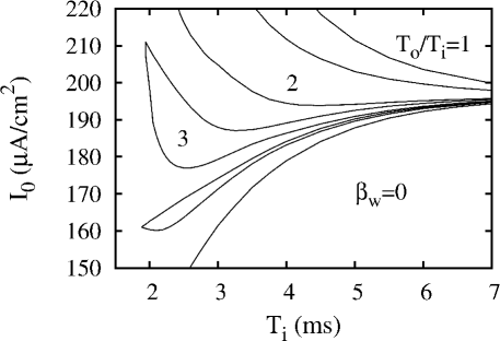
Figure 1: Response diagram for $\beta_{w}=0$. The main locked-in states, 1:1, 2:1, and 3:1, are labeled by the inverse of the firing rate, $T_{o}/T_{i}$, where the $T_{o}$ is the average time between voltage spikes. The 4:1 state is also shown but its label is omitted due to a lack of space. The lowest line is the excitation threshold between quiescence and a finite firing rate.

Figure 1 shows the global bifurcation diagram in the period-amplitude plane for $\beta_{w}=0$. We call it a response diagram since it characterizes the response of the dynamical system to a periodic perturbation. The lines on this graph are borders between the dominant locked-in states and regions of irregular response. In the limit, where $I_{app}$ is always constant and $T_{i}=\tau$, this choice leads to type 1 excitability Prescott2008 . In Fig. 1 the dependence of the firing rate $f_{o}/f_{i}$ on $I_{0}$, where $f_{i}=1/T_{i}$, and $f_{o}=1/T_{o}$, is continuous everywhere along the excitation threshold, scaling approximately as $(I_{0}-I_{th})^{1/2}$, where $I_{th}$ is the value of $I_{0}$ at the threshold.

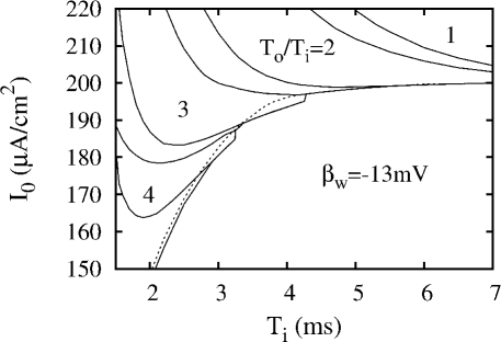
Figure 2: Response diagram for $\beta_{w}=-13\textrm{mV}$. The locked-in states of order 3:1 and higher are bistable along the threshold. However the 2:1 state remains monostable. The dashed line separates the monostable regime from the bistable area. We have verified that MMT does not appear in this case.

When $\beta_{w}=-13\textrm{mV}$, the neuron displays class 2 dynamics for a constant current. In Fig. 2 we can see that the firing rate is a discontinuous function of the current amplitude also at short stimulation periods. For $T_{i}<4\textrm{ms}$ almost the entire threshold is bistable. However, for $T_{i}>4\textrm{ms}$ the system remains monostable. More precisely, the bistability does not extend beyond the 3:1 state and the edge of the 2:1 state is monostable. The long-period response in Figs. 1 and 2 is very similar. Wang et al. Wang2011 also noted the similarity of response in this regime for a sinusoidal input.

Figure 3: Response diagram for $\beta_{w}=-23\textrm{mV}$. The dashed line separates the monostable regime from the bistable area. The location of the odd-all multimodal transition is denoted by full squares. For $1.5\textrm{ms}<T_{i}<5\textrm{ms}$ this diagram closely resembles the one obtained for the HH model Borkowski2011 .

Fig. 3 shows the response diagram for $\beta_{w}=-23\textrm{mV}$. There are now large bistable regions of the states 3:1 and 2:1. The short stimulation period part of the diagram, for $T_{i}<5\textrm{ms}$, closely resembles the regime of the HH model where the MMT occurs Borkowski2009 ; Borkowski2010 . We have analyzed the histogram of interspike intervals (ISI) and found the same dynamic singularity in the ML model. The location of the transition is indicated in Fig. 3 by full squares. The $f_{o}$ vs $I_{0}$ dependence in the interval between the MMT and the 2:1 state is approximately linear, as in the HH model Borkowski2009 . The MMT along the $T_{i}$ axis for $\beta_{w}=-23\textrm{mV}$ is shown in Fig. 4.

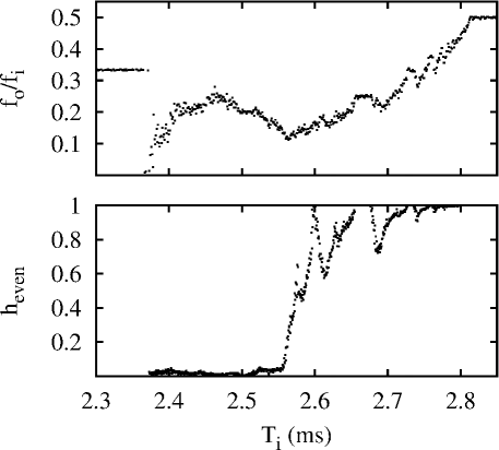
Figure 4: The firing rate (top) and the weight of even modes (bottom) for $\beta_{w}=-23\textrm{mV}$ and $I_{0}=245\mu\textrm{A/cm}^{2}$.

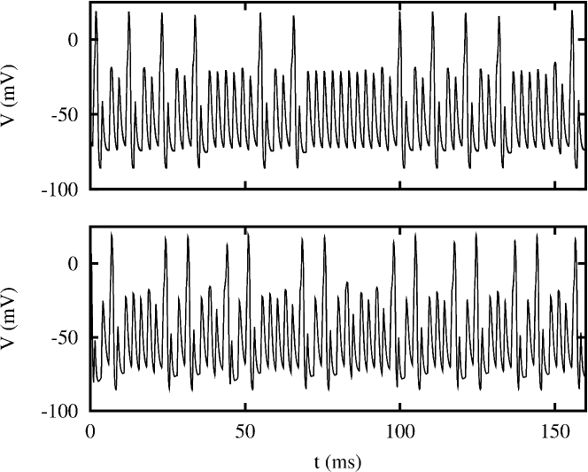
Figure 5: Sample $V(t)$ run for $\beta_{w}=-23\textrm{mV}$, $I_{0}=245\mu\textrm{A/cm}^{2}$. The top panel contains data taken above the odd-all transition at $T=2.65\textrm{ms}$. Here the even modes are more frequent than the odd ones but there is also some admixture of the odd modes. The bottom panel shows data at $T_{i}=2.45\textrm{ms}$. Note the absence of even multiples of the driving period in the bottom panel. Here the response contains only the following multiples of $T_{i}$: 3, 5, 7, and 9.

The weight of even modes drops sharply in the vicinity of the minimum of the firing rate. The edges of individual modes near the transition scale logarithmically, as in the HH model Borkowski2009 . All these signatures of the MMT and the topology of the bifurcation diagram in the vicinity of the MMT in the ML model are identical to the HH model.

Fig. 5 shows sample $V(t)$ runs on both sides of the even-all transition. In the top panel, obtained at $T_{i}=2.65\textrm{ms}$, the even modes 4:1 and 8:1 dominate. In the bottom panel obtained at $T_{i}=2.45\textrm{ms}$ only odd modes are present. Here the height of the $V(t)$ peak correlates with the length of the preceding interspike interval. A careful examination of the peak heights reveals a preference for a $T_{o}=3T_{i}$, following the action potential with the maximum value of $V$. This preference is manifested either as (i) another action potential, or as (ii) subthreshold peak with a height somewhat larger than that of its immediate neighbors. Judging by the height of subthreshold peaks there is a clear preference for a period $2T_{i}$ subthreshold oscillation. We can view the odd-only periods in the bottom panel as a sum of $3T_{i}+2nT_{i}$, where $n=0,1,\ldots$.

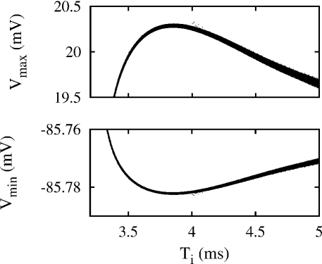
Figure 6: Maximum and minimum values of $V(t)$ as a function of $T_{i}$ for $\beta_{w}=-23\textrm{mV}$ and $I_{0}=230\mu\textrm{A/cm}^{2}$. It is a cross section of the 2:1 mode-locked area. The optimal response is obtained at $T_{i}\simeq 3.85\textrm{ms}$, which gives the resonant time scale of $7.7\textrm{ms}$.

The system’s resonant frequency may be estimated by examining the extrema of $V(t)$. Fig. 6 shows the dependence of $V_{max}(t)$ and $V_{min}(t)$ on stimulus period in the 2:1 zone of Fig. 3. The action potential amplitude reaches maximum values at $T_{i}\simeq.85\textrm{ms}$. Therefore the resonant period is $T_{res}\simeq 2\times 3.85\textrm{ms}=7.7\textrm{ms}$, giving the resonant frequency of $f_{res}=1/7.7\textrm{ms}=130\textrm{Hz}$. A similar estimate, although somewhat less accurate, is obtained from the minimum of the monostable region of the 2:1 zone in Fig. 3 located near $T_{i}=3.5\textrm{ms}$. For other values of $\beta_{w}$, $f_{res}$ can be obtained also from the minimum thresholds of the 3:1 and 4:1 zones in Figs. 1 and 2. We found that $f_{res}$ does not depend significantly on $\beta_{w}$.

We also analyzed the ISI histogram as a function of $\beta_{w}$, looking for signs of the MMT. For $\beta_{w}=-13\textrm{mV}$ we can see a precursor of the odd-all MMT in Fig. 7. There is a local minimum of $f_{o}/f_{i}$ at $I_{0}=198.2\mu\textrm{A/cm}^{2}$ and a significant decrease of the participation rate of even modes close to the threshold.

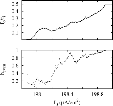
Figure 7: The firing rate and the joint histogram weight of even modes for $\beta_{w}=-13\textrm{mV}$ and $T_{i}=4.7\textrm{ms}$. A precursor of the multimodal transition can be seen near $I_{0}=198.2\mu\textrm{A/cm}^{2}$. There is a well pronounced local minimum of the $f_{o}/f_{i}$ and a significant reduction of the participation rate of even modes.

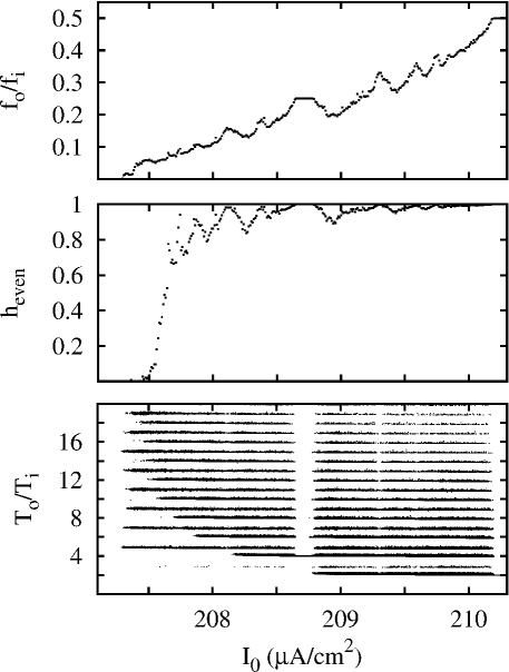
Figure 8: From top to bottom: the firing rate, the joint histogram weight of even modes, and the ISI spectrum for $\beta_{w}=-18\textrm{mV}$ and $T_{i}=3.7\textrm{ms}$. The multimodal transition occurs at $I_{0}=207.5\mu\textrm{A/cm}^{2}$.

The MMT is tied to the appearance of bistability along the bottom edge of the 2:1 state, which occurs for $\beta_{w}<-14.5\textrm{mV}$. In Fig. 8 we can see that for $\beta_{w}=-18\textrm{ms}$ the MMT is already well developed. As the MMT is approached from above, only very high order even modes remain. The edges of the even modes scale logarithmically as a function of $|I_{0}-I^{*}|$, where $I^{*}$ is the current amplitude at which the transition occurs. When the bistability of the state 2:1 disappears near $\beta_{w}=-29\textrm{mV}$, so does the MMT. At this value of $\beta_{w}$ the 3:1 state vanishes from the global bifurcation diagram.

III Conclusions

The dynamics of neurons at periods below the resonant period is not directly related to either class 2 or class 3 excitability. The global bifurcation diagram of the class 3 ML model for $\beta_{w}=-23\textrm{mV}$ closely resembles the class 2 HH model Borkowski2009 at intermediate periods. This is consistent with the remarks of Prescott et al. Prescott2008 that neurons should not be labeled as being strictly type 2 or type 3. The transition to bistability at the edge of a 2:1 state in a model stimulated by a train of current pulses does not occur for the same parameter values as the transition to bistability for a constant current. The bistability appears first in the limit of small stimulation period. As $\beta_{w}$ decreases further, the perithreshold regions for larger $T_{i}$ also become bistable. The MMT occurs when both the 2:1 and the 3:1 state have bistable regions along the threshold. The ability to predict the existence of the MMT from the topology of the locked-in states in the perithreshold regime is of course a very useful property. Testing for bistabilities near the threshold is much simpler and computationally much more efficient than analyzing the evolution of the entire ISI histogram as a function of pulse period or amplitude.

Wang et al. Wang2011 noted the similarity of class 1 and class 2 neuron response to sinusoidal signal at low frequencies. This is not surprising, once we note, that the threshold bistability, and a discontinuity of the firing rate $f_{o}/f_{i}$ associated with it, appears first in the limit of small $T_{i}$ and extends towards larger $T_{i}$ with decreasing $\beta_{w}$. When $\beta_{w}<-14.5\textrm{mV}$, the 3:1 state becomes bistable and the entire threshold in the regime of small $T_{i}$ rises significantly. The emergence of class 3 behavior may be viewed as a strong rigidity of neuron dynamics in the limit of high stimulation period.

Based on this relationship between MMT and the global bifurcation diagram we can classify neuron excitability for stimuli of finite frequency: (i) class 1, where the firing rate is a continuous function of $I_{0}$ everywhere along the threshold, (ii) class 2, with bistabilities at the edges of high-order locked-in states, (iii) class 3, where the MMT exists, and (iv) class 4, where both the MMT and the bistabilities are absent and the neuron responds to a constant current by emitting only a few spikes.

The presence of the MMT in both the ML and HH model suggests that the same transition is present in other resonant neuron models classified as type 2 or type 3 cells. The existence of MMT may have important physiological consequences. It may be relevant in the high-frequency auditory nerve fiber stimulation OGorman2009 and possibly in the clinical procedure of deep brain stimulation McIntyre2000 .

References

References

- (1) A. L. Hodgkin, J. Physiol. (London) 107 165 (1948).
- (2) H. R. Wilson, Spikes decisions, and actions: The dynamic foundations of neuroscience, Oxford University Press (1999).
- (3) J. A. Connor, D. Walter, and R. McKown, Biophys. J. 18, 81 (1977).
- (4) G. B. Ermentrout, Neural Comput. 8, 979 (1996).
- (5) G. B. Ermentrout and N. Kopell, SIAM J. Appl. Math. 46, 233 (1986).
- (6) G. F. Hoppensteadt and E. M. Izhikevich, Weakly connected neural networks, Springer (New York, 1997).
- (7) B. S. Gutkin and G. B. Ermentrout, Neural Comput. 10, 1047 (1998).
- (8) X.-J. Wang and G. Buzsáki, J. Neurosci. 16, 6402 (1996).
- (9) A. L. Hodgkin and A. F. Huxley, J. Physiol. (London) 117, 500 (1952).
- (10) T. Tateno, A. Harsch, and H. P. C. Robinson, J. Neurophysiol. 92, 2283 (2004).
- (11) T. Tateno and H. P. C. Robinson, J. Neurophysiol. 95, 2650 (2006).
- (12) C. Morris and H. Lecar, Biophys. J. 35, 193 (1981).
- (13) J. Rinzel and G. B. Ermentrout, In: C. Koch and I. Segev, eds. Methods in Neuronal Modeling: from Ions to Networks. Cambridge (Massachusetts): The MIT Press, pp. 251-291.
- (14) J. L. Hindmarsh and R. M. Rose, Proc. R. Soc. London B 221, 87 (1984).
- (15) S. A. Prescott, Y. De Koninck, and T. J. Sejnowski, PLoS Comput. Biol. 4, e1000198 (2008).
- (16) J. R. Clay, J. Neurophysiol. 80, 903 (1998).
- (17) J. R. Clay, Prog. Biophys. Mol. Biol. 88, 59 (2005).
- (18) J. R. Clay, D. Paydarfar, and D. B. Forger, J. R. Soc. Interface 5, 1421 (2008).
- (19) L. S. Borkowski, Phys. Rev. E 83, 051901 (2011).
- (20) H. S. Strogatz, Nonlinear Dynamics and Chaos, Perseus (Cambridge, 1994).
- (21) L. S. Borkowski, Phys. Rev. E 80, 051914 (2009).
- (22) N. Takahashi, Y. Hanyu, T. Musha, R. Kubo, and G. Matsumoto, Physica D 43, 318 (1990).
- (23) L. S. Borkowski, Phys. Rev. E 82, 041909 (2010).
- (24) M. St-Hilaire and A. Longtin, J. Comput. Neurosci. 16, 299 (2004).
- (25) R. Naud, N. Marcille, C. Clopath, and W. Gerstner, Biol. Cybern. 99, 335 (2008).
- (26) L. S. Borkowski, arXiv.org:1105.5376 [physics.bio-ph].
- (27) H. Wang, L. Wang, L. Yu, and Y. Chen, Phys. Rev. E 83, 021915 (2011).
- (28) D. E. O’Gorman, J. A. White, and C. A. Shera, J. Assoc. Res. Otolaryngol. 10, 251 (2009).
- (29) C. C. McIntyre and W. M. Grill, Ann. Biomed. Eng. 28, 219 (2000).