Properties of Doubly Stochastic Poisson Process with affine intensity

Abstract

This paper discusses properties of a Doubly Stochastic Poisson Process (DSPP) where the intensity process belongs to a class of affine diffusions. For any intensity process from this class we derive an analytical expression for probability distribution functions of the corresponding DSPP. A specification of our results is provided in a particular case where the intensity is given by one-dimensional Feller process and its parameters are estimated by Kalman filtering for high frequency transaction data.

1 Introduction

The Doubly Stochastic Poisson Processes (DSPPs) were introduced by Cox (1955) by allowing the intensity of the Poisson process to be described by a positive random variable and not just a deterministic function. The aim of such a generalization was to allow the dynamic of a process that is exogenous to the model to influence transitions in the point process that we are concerned with. Point processes have applications in several areas of applications, among which we mention: biostatistics, finance and reliability theory. In biostatistics they form a theoretical framework for studying recurrent events, as was done in Gail et al. (1980), in studies of the size of tumors in rats over a period of time. In finance, Lando (1998) was the pioneer in using point processes for describing occurrences of credit events. In reliability theory, Dalal and McIntosh (1994) work has developed criteria for determining an optimum stopping time for testing and validating a software.

It was the seminal work by Cox (1955) which introduced the DSPPs (also known as the Cox Process). The main work in this field is Grandell (1976) where the main properties of the DSPPs have been presented in terms of standard construction of Probability Theory. Alternatively, in the books of Brémaud (1972) and Daley and Vere-Jones (1988) the presentation is based in line with the concepts and properties of Martingales. However, all these sources focus on deriving general properties of DSPP, without exploring the functional form of the intensity of the process. Consequently, they attracted a reduced number of applications.

The study of the DSPPs took a new turn once the functional form for the intensity of the process has been specified. As a result it became possible to obtain analytical expressions for probability density functions for different types of processes. In this context we can quote may be cited Bouzas et al. (2002) who made use of truncated normal distribution to describe the intensity of the process and Bouzas et al. (2006) who generalized the form of intensity to include the case of a harmonic oscillator. The contribution of these works was that closed analytical expressions for density functions of the Cox process have been obtained, as well as their moments. However, in both cases the authors used constructions in which the restriction on non-negativity for the intensity measure was not maintained. In order to get a round of this limitation, the authors defined a region in the parameter space where the probability of occurrence of negative values for the intensity is reduced. With the intent to guarantee the preservation of the non-negativity condition, Basu and Dassios (2002) and Kozachenko and Pogorilyak (2008) suggested the adoption of a lognormal model for the process intensity. A formulation that incorporates the intensity into a dynamic formulation is developed in Dassios and Jang (2008) who use the functional form of a process of the Shot-Noise type which, despite guaranteeing the non-negativity of intensity, is not in fact a diffusion process. On the other hand Wei et al. (2002) assumed that the intensity is governed by a one-dimensional Feller process and obtained a form of probability density function for the corresponding DSPP.

Feller processes were introduced and established in the financial literature after Cox et al. (1985). One of the properties is that the Feller process lives in $\mathbb{R}_{+}$ which guarantees that the non-negativity condition is fulfilled. In the present work we assume that the intensity is controlled by a related diffusion process, as formalized by Duffie and Kan (1996), which incorporates Feller processes in one or $d$ dimensions. In this way, the models from Wei et al. (2002), Basu and Dassios (2002) and Kozachenko and Pogorilyak (2008) can be seen as specific examples of the model proposed in the present work.

The use of point processes in finance, especially of DSPPs, progressed considerably at the end of the 1990s with the development of models of managing and pricing the credit risk. In particular, Duffie and Singleton (1999) and Duffie et al. (2003) formalized the construction of the probability density of the first jump in the process, in a related context. More precisely, the time to the first jump represents, in the context of credit risk, the time until the bankruptcy (default) of a company (and/or a country). Here, once the absorbing state had been reached, it was unnecessary to study the further dynamic of the DSPP.

Recently a new area of applications of point processes in finance has emerged, along with the use of these models for describing the arrival process of bid and ask orders in an electronic trading environment. In these models, the arrival process of orders changes over time; the idea is to characterize the dynamic of this process and obtain expressions that may be treated analytically, describing the probability that an order had been sent in line with a market configuration and was executed before the price was altered. See Cont et al. (2010).

Perhaps the most well known point process is the homogenous Poisson process. For this process the arrival rate is constant. A homogenous Poisson process can therefore be described by a single value $\lambda_{t}=\lambda$. However, in many applications the assumption of a constant arrival rate is not realistic. Indeed, in financial data we tend to observe bursts of trading activity followed by lulls. This feature becomes apparent when looking at the series of actual orders arrivals. Figure 1 presents the average number of sell orders for BRL/USD FX futures submitted to the Brazilian Exchange, BVMF. The plot indicates a non-constant behavior for the average number of submitted orders; the homogenous Poisson model is clearly not suitable for such data.

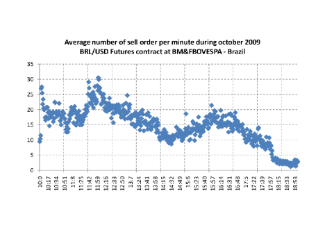
Figure 1: Sell orders for FX futures contract during October: (ticker DOL FUT - expiry NOV09)

In fact, the number of bids and asks that getting into the order book may depend upon a number of factors exogenous to the model. For example, it may be the level of investors risk aversion on a given day, or intra-day seasonality, or a disclosure of a piece of information, or a new technology producing an impact on a certain sector of the economy. For this reason, in our opinion, the construction of a model that can be treated analytically and incorporates endogenously a stochastic behavior of the intensity of a point process represents a contribution to the literature. In light of the above topics, the main aim of this article is to present new results on DSPPs when the intensity belongs to a family of so-called affine diffusions with potencial application in high frequency trading.

In this situation seems reasonable to focus on a particular class of models and attempt to use the approach based on point processes in order to study their dynamic over time. For this purpose we selected the Affine Term Structure (ATS) models, and our goal is to obtain the form Theorem for the Probability Density Functions for the Cox Process when the intensity belongs to a family of affine diffusion. Additionally, in one particular case when the intensity is governed by an one-dimensional Feller diffusion we obtain more detailed results, such as its moments and the convergence to its stationary distribution. Finally we propose an estimation procedure for point processes with stochastic affine intensity based on Kalman Filter conjugated with quasi-maximum likelihood estimator. Thus, the estimation procedure is applied to high frequency transactional data from FX futures contracts traded in Brazil.

2 The basic structure

Consider the filtered probability space $\left(\Omega,\mathcal{G},\mathbb{G},\mathbb{P}\right)$, where $\mathbb{G}=(\mathcal{G}_{t})_{t\geq 0}$ is a filtration having the sets with null measure and right continuous.

Definition 1

Let $\tau$ be a non-negative random variable $\tau:\Omega\rightarrow\mathbb{R}^{+}\cup\infty$, which is defined on a probability space $\left(\Omega,\mathcal{G},\mathbb{G},\mathbb{P}\right)$, such that $\{\tau\leq t\}\in\mathcal{G}_{t}\hskip 8.5359pt\forall t\geq 0$.

Definition 2

Given a no-decreasing sequence of stopping time $\{\tau_{i},i\in\mathbb{N}\}$, the Point Processes $N_{t}$ is a (càdlàg) processes defined as:

$$N_{t}:=\displaystyle\sum_{i}1\hskip-2.5pt\hbox{I}_{\{\tau_{i}\leq t\}}$$ (1)

Definition 3

Define the intensity processes as:

$$\lambda_{t} =\rho_{0}+\sum_{i=1}^{d}\rho_{i,1}X_{i,t}$$ (2)

$$=\rho_{0}+\rho_{1}\cdot X_{t}$$ (3)

With $\rho_{0}\in\mathbb{R}$ and $\rho_{1}\in\mathbb{R}^{d}$. Where the state variable $X_{t}$ will be defined below.

Definition 4

Let $\left(\Omega,\mathcal{G},\mathbb{G},\mathbb{P}\right)$ be a filtered probability space and let $\mathbb{F}$ be a sub-filtration of $\mathbb{G}$. We called cumulate intensity (or Hazard Process) an $\mathcal{F}$-adapted, right-continuous, increasing stochastic process $\Lambda_{0,t}=\int_{0}^{t}\lambda_{u}du$ for $t\geq 0$ with $\mathbb{P}$-a.s. $\Lambda_{0}=0$ and $\Lambda_{\infty}=\infty$.

The hazard process plays an important role in the martingale approach to either credit risk or asset pricing because it is the compensator of the associated doubly stochastic Poisson process, see for example Bielecki and Rutkowski (2002). For our purposes, the hazard process will be important to derive the probability density function for the Point Process, $(N_{t})_{t\geq 0}$. To construct the stopping time with the given intensity, define as in Lando (1998):

$$\tau_{i}:=\inf\Bigl{\{}t:\Lambda^{i}_{0,t}\geq E_{1,i}\Bigr{\}}$$ (4)

where $E_{1,i}$ is a unit exponential random variable independent of $X_{t}$ $\forall$ i.

Definition 5

Let $X_{t}:\mathcal{D}\times\mathbb{R}\rightarrow\mathbb{R}^{d}$, be the state variable as solution for the stochastic differential equation SDE:

$$dX_{t}=\mu(X,t)dt+\sigma(X,t)dW_{t}$$ (5)

where: $\mu(X,t):\mathcal{D}\times\mathbb{R_{+}}\rightarrow\mathbb{R}^{d}$, is the drift; $\sigma(X,t):\mathcal{D}\times\mathbb{R}_{+}\rightarrow\mathbb{R}^{d\times d}$, the diffusion coefficient and, $W_{t}$ the standard Brownian Motion defined in $\left(\Omega,\mathcal{G},\mathbb{G},\mathbb{P}\right)$. Where $\mathcal{D}\subset\mathbb{R}^{d}$ will be properly defined below.

Definition 6 (Duffie and Kan (1996))

Define $X_{t}$ as an affine processes, if the following condition are simultaneously satisfied for (5):

1. Drift

   $$\mu(X,t)=\mathcal{K}(\Theta-X_{t})$$ (6)

   For $\Theta\in\mathbb{R}^{d}$ and $\mathcal{K}\in\mathbb{R}^{d\times d}$

2. Covariance matrix

   $$\sigma(X,t)=\Sigma\sqrt{\sigma}$$ (7)

Where $\Sigma$ is $d\times d$ matrix not necessarily symmetric, and $\sigma$ is a diagonal matrix with the i-th elements from the diagonal given by:

$$\sigma_{i}=a_{i}+b_{i}X_{t},\hskip 14.22636pti=1,\ldots,d,$$ (8)

with a $\in\mathbb{R}$ e $b\in\mathbb{R}^{d}$.

Adopting the construction of Duffie and Kan (1996) and Dai and Singleton (2000) the state variable in its affine form is:

$$\mbox{d}X_{t}=\mathcal{K}(\Theta-X_{t})dt+\Sigma\sqrt{\sigma}\mbox{d}W_{t}$$ (9)

where $W_{t}$ is the d-dimensional independent standard Brownian Motion in $\left(\Omega,\mathcal{G},\mathbb{G},\mathbb{P}\right)$, $\mathcal{K}$ and $\Sigma$ are $d\times d$ matrices which may be nondiagonal and asymmetric.

According to Duffie and Kan (1996) the coefficient vectors $b_{1},\ldots,b_{d}$ in (8) generate stochastic volatility unless they are all zero, in which case (9) defines a Gauss-Markov process. If the volatilities (all or some) are stochastic, then two questions face up: how to constrain the model in order to avoid negative volatilities? Under those constraints, which is the set $\mathcal{D}\subset\mathbb{R}^{d}$ where the process $(X_{t})_{t\geq 0}$ can take values?
The open domain $\mathcal{D}$ implied by nonnegative volatilities may be defined as:

$$\mathcal{D}=\bigg{\{}x\in\mathbb{R}^{d}:a_{i}+b_{i}\cdot x\geq 0,\hskip 14.22636pti\in\{1,\ldots,d\}\bigg{\}}$$ (10)

The following condition of Duffie and Kan (1996) is sufficient for the positiveness of $\sigma_{i}$:

Condition A (Duffie and Kan (1996)): For all i:

1. $\forall x\hskip 8.5359pt\mbox{such that}\hskip 8.5359pt\sigma_{i}(x)=0,\hskip 8.5359ptb_{i}^{\top}(\mathcal{K}(\Theta-X_{t})>\frac{1}{2}b_{i}^{\top}\Sigma\Sigma^{\top}b_{i}$

2. $\forall j,\hskip 8.5359pt\mbox{if}\hskip 8.5359pt(b_{i}^{\top}\Sigma)_{j}\neq 0$, then $\sigma_{i}=k\sigma_{j}$ for $k>0$

Both parts of Condition A are designed to ensure strictly positive volatility, and they are both effectively necessary for this purpose.

A second set of constrains must be imposed to guarantee that the non-negativity condition for $(\lambda_{t})_{t\geq 0}$ is fulfilled. The open domain $\mathcal{D}$ implied by nonnegative intensities may be defined as:

$$\mathcal{D}=\bigg{\{}x\in\mathbb{R}^{d}:\lambda_{t}(x)\geq 0\bigg{\}}$$ (11)

In this sense, the strongest form of guarantee that (10) and (11) are simultaneously met it is to impose $\mathcal{D}=\mathbb{R}^{d}_{+}$. However, it is a very strong constraint on the state space resulting in a large number of models excluded.

Using the Canonical Representation developed by Duffie and Singleton (1999) it will be possible to overcome the non-negativity for $(\lambda_{t})_{t\geq 0}$. In fact, according to the Canonical Representation, $\mathbb{A}_{m}(d)$, where $m=rank(\sigma)$, the state vector $X_{t}$ will be split into two subvectors: the first factors vector $X_{t}^{B}\in\mathbb{R}^{m}$, with $0\leq m\leq d$ and the other group of factors are stacked in $X_{t}^{D}\in\mathbb{R}^{d-m}$.

This way it is also possible to overcome existence and uniqueness problems for a more general class of affine diffusion than the one that satisfies (9). In fact the process $X_{t}^{B}$ exists and is unique, moreover it is autonomous with respect to $X_{t}^{D}$. The volatility of $X_{t}^{D}$, conditionally on $X_{t}^{B}$, is given, so there is no uniqueness problem concerning $X_{t}^{D}$. Finally, from the Canonical Representation it is known that the process $X^{D}$, when $X^{D}\neq 0$, has Gaussian Distribution, independent from $X^{B}$, with mean $\mu^{D}$ and standard deviation $\sigma^{D}$.

From the Canonical Representation, we just need to impose an extra condition to ensure strictly positive of $(\lambda_{t})_{t\geq 0}$.

Condition B: if we set

$$\mu^{D}>0\hskip 2.84544pt,$$ (12)

it is possible to state that:

Proposition 1

If $\gamma^{*}\mu^{D}>\sigma^{D}$, then the process $X^{D}$ is nonnegative almost sure, i.e. $X^{D}\in\mathcal{D}^{+}$.

Proof of Proposition 1

According to the Canonical Representation, the process $X^{D}$ is Gaussian with mean $\mu^{D}$ and standard deviation $\sigma^{D}$. Thus it is possible to compute the probability $X^{D}\in\mathcal{D}^{+}$:

$$\mathbb{P}(X^{D}>0)=\Phi\left(\frac{\mu^{D}}{\sigma^{D}}\right)$$ (13)

where $\Phi(\cdot)$ is the cumulative normal distribution function.

Because condition (12) the problem described in (13) is now written as:

$$\gamma^{*}=\displaystyle\inf_{\gamma}(\gamma:\Phi(\gamma)=1)$$ (14)

where: $\gamma=\frac{\mu^{D}}{\sigma^{D}}$

Then by requiring that $\gamma^{*}\mu^{D}>\sigma^{D}$ the non-negativity condition for $(\lambda_{t})_{t\geq 0}$ is satisfied almost sure.

$\blacksquare$

We now turn to examples and illustrations of Affine framework.

• Example 1

  : Ornstein-Ulhenbeck (Vasicek)

  $$dX_{t}=\kappa(\theta-X_{t})dt+\sigma dW_{t}$$

• Example 2

  : Feller (or Square Root, Cox-Ingersoll-Ross)

  $$dX_{t}=\kappa(\theta-X_{t})dt+\sigma\sqrt{X_{t}}dW_{t}$$

• Example 3

  : Geometric Brownian Motion

  $$\frac{dS_{t}}{S_{t}}=\mu dt+\sigma dW_{t}$$

  $$X_{t}:=lnS_{t}\hskip 28.45274ptdX_{t}=\left(\mu-\frac{1}{2}\sigma^{2}\right)dt+\sigma dW_{t}$$

• Example 4

  : Heston (Stochastic Volatility)

  $$X_{t}:=lnS_{t}\hskip 28.45274ptdX_{t}=\left(\mu-\frac{1}{2}\sigma^{2}_{t}\right)dt+\sigma_{t}dW^{1}_{t}$$

  
  

  $$d\sigma_{t}=\kappa(\theta-\sigma_{t})dt+\nu\sqrt{\sigma_{t}}dW^{2}_{t}$$

  
  

  $$<dW^{1}_{t},dW^{2}_{t}>=\rho$$

• Example 5

  : Multivariate CIR

  $$dX_{t}=\left(\left[\begin{array}[]{c}\kappa_{1}\theta_{1}\\ \kappa_{2}\theta_{2}\\ \end{array}\right]+\left[\begin{array}[]{cc}-\kappa_{1}&0\\ 0&-\kappa_{2}\\ \end{array}\right]X_{t}\right)dt+\left[\begin{array}[]{cc}\sigma_{1}&0\\ 0&\sigma_{2}\\ \end{array}\right]\left(\sqrt{\left[\begin{array}[]{cc}1&0\\ 0&1\\ \end{array}\right]X_{t}}\right)dW_{t}$$

In order to have the no-negative random variable $\tau_{i}$ as a stopping time a technical conditions must be imposed over the filtration. So we shall first examine a trivial case where the condition is not respected.

Proposition 2

The hitting time $\tau$ is not a $\mathbb{F}$-stopping time with respect to $\mathcal{F}_{t}:=\sigma\{W_{s}:0\leq s\leq t\}$

Proof of proposition 2
Assume, by absurd, that $\tau$ is $\mathbb{F}$-stopping time for $\mathcal{F}_{t}:=\sigma\{W_{s}:0\leq s\leq t\}$, so using the Martingale Representation Theorem there exist a compensated process (a $\mathbb{F}$-Martingale) $M_{t}$ which may be represented as a stochastic integral with respect to the Brownian motion $W$. Therefore we arrive a contradiction because $M_{t}$ must jump in $\tau$.

$\blacksquare$

Thus the filtration $\mathbb{F}$ should be enlarge. There are several ways to expand it but we do enlarged $\mathbb{F}$ just to get $\tau$ as stopping time. Then the proper filtration $\mathbb{G}=(\mathcal{G}_{t})_{t\geq 0}$ will be constructed as:

$$\mathcal{G}_{t}=\mathcal{F}_{t}\vee\mathcal{H}_{t}$$

where

$$\mathcal{H}_{t}=\sigma\{N_{s}:0\leq s\leq t\}$$

Definition 7

Let $\left(\Omega,\mathcal{G},\mathbb{G},\mathbb{P}\right)$ be a filtered probability space and $N_{t}$ a stochastic processes defined on it. Let $\mathbb{F}$ be a sub-filtration of $\mathbb{G}$, then $N_{t}$ is called a Doubly Stochastic Poisson Process with relation to $\Lambda_{t}$, if $\lambda_{t}$ is $\mathbb{F}$-measurable and for all $0\leq t\leq T$ and $k=0,1,\ldots$ the next condition be satisfied:

$$P(N_{T}-N_{t}=k|\mathcal{H}_{t}\vee\mathcal{F}_{\infty})=\frac{1}{k!}\left(\Lambda_{t,T}\right)^{k}\exp\left(-\Lambda_{t,T}\right)$$ (15)

where $\mathcal{F}_{\infty}=\sigma(\mathcal{F}_{u}:u\in\mathbb{R}_{+})$

As a particular case:

$$P(N_{T}-N_{t}=k|\mathcal{H}_{t}\vee\mathcal{F}_{\infty})=P(N_{T}-N_{t}=k|\mathcal{F}_{\infty})$$ (16)

Therefore, conditioned to $\sigma$-field $\mathcal{F}_{\infty}$ the increments of $N_{T}-N_{t}$ are independent of the $\sigma$-field $\mathcal{H}_{t}$.

Thus, the probability of no occurrences within the interval $[t,T]$ for the processes $N_{t}$ with intensity $\lambda_{t}>0$ is given by:

$$P(N_{T}-N_{t}=0)=\mathbb{E}_{t}\left[\exp\left(-\int_{t}^{T}\lambda_{u}du\right)\right]$$ (17)

2.1 Laplace transform for the process $\Lambda_{t}$

The Laplace transform of stochastic processes is a key ingredient to achieve our results. However Laplace transform for integral of stochastic processes may be obtained in closed form only for a limited number of processes.

Albanese and Lawi (2004) formalize the criteria to define which processes have a analytic form for its Laplace transform. Thus take a diffusion $(X_{t})_{t\geq 0}$ defined on $\left(\Omega,\mathcal{G},\mathbb{G},\mathbb{P}\right)$ and consider the Laplace transform defined by:

$$L_{t}(\mu,X,t):=\mathbb{E}_{t}\left[f(X,s)\exp\left(-\mu\int_{t}^{T}\phi(X,s)ds\right)\bigg{|}\mathcal{G}_{t}\right]$$ (18)

where $t\leq T$, $\mu\in\mathbb{C}$ and $f,\phi:\mathbb{R}\mapsto\mathbb{R}$ two Borel functions.

Thus, it is possible to state that:

Result 1 (Albanese and Lawi (2004))

The class of stochastic processes with Laplace transform for its integral is given by:

$$dX_{t}=2\frac{h^{\prime}(X_{t})}{h(X_{t})}\frac{A(X_{t})^{2}}{R(X_{t})}dt+\frac{\sqrt{2}A(X_{t})}{\sqrt{R(X_{t})}}dW_{t}$$ (19)

With additional conditions:

1. Three second order polyonymous in x: $A(x)$,$R(x)$,$Q(x)$. Such that $A(x)$ belongs to the set o $\{1,x,x(1-x),x^{2}+1\}$ e $R(X_{t})\geq 0$;

2. The function $h(x)$ is a linear combination of hypergeometric functions of the confluent

   From type ${}_{1}F_{1}$ if $A(x)\in\{1,x\}$ and gaussian from type ${}_{2}F_{1}$ otherwise.

Thus the Laplace Transform $L_{t}(\mu,X,t)$ is defined by:

$$\phi(x)=\frac{Q(x,\mu)}{\mu R(x)}$$ (20)

Example 6

: As an application from the above result we shall prove that the Laplace transform of $\Lambda_{t}:=\int_{0}^{t}\lambda_{u}du$ when the intensity follows a one-dimension Feller process exists.

Thus assume that the polynomials are defined as:

$$A(x)=x,\hskip 14.22636ptR(x)=\frac{2x}{\sigma^{2}},\hskip 14.22636pth(x)=x^{a/\sigma^{2}}e^{-\frac{b}{\sigma^{2}}x}$$ (21)

Substituting the polynomial into (19) with a variable change we have:

$$d\lambda_{t}=\kappa(\theta-\lambda_{t})dt+\sigma\sqrt{\lambda_{t}}dW_{t}$$

So in those cases where the Laplace transform $L_{t}(\mu,X,t)$ exists it is possible to apply the well know result:

Result 2 (Feynman-Kac)

Let $(X_{t})_{t\geq 0}$ be a diffusion process with infinitesimal generator $\mathcal{A}$. Assume that $F\in C^{2,1}(\mathcal{D}^{d}\times[0,t))$ and $V\in C^{1}$ is bounded. Then:

$$F(x,t,\mu)=\mathbb{E}_{t}\left[f(X_{t})\exp\left(-\mu\int_{t}^{T}V(x,s)ds\right)\bigg{|}\mathcal{G}_{t}\right]$$ (22)

it is solution of the partial differential equation (PDE):

$$\left\{\begin{array}[]{rcl}\frac{\partial F}{\partial t}&=&\mathcal{A}F(x,t,\mu)-V(x,t)F(x,t,\mu))\\ F(x,0,\mu)&=&f(x)\hskip 14.22636ptx\in\mathcal{D}\end{array}\right.$$ (23)

and

$$\mathcal{A}F(x,t)=\frac{\partial F}{\partial t}+\frac{\partial F}{\partial x}\mu(x,t)+\frac{1}{2}\mbox{Tr}\bigg{[}\sigma(x,t)\sigma(x,t)^{\top}\frac{\partial^{2}F(t,x)}{\partial X\partial X}\bigg{]}$$ (24)

Furthermore , if $U(x,t,\mu)\in C^{2,1}$ solve (23), then $U(x,t,\mu)=F(x,t,\mu)$.

Taking the Theorem 2 it is possible to state that:

Proposition 3

Let $(X_{t})_{t\geq 0}$ be a diffusion processes satisfying the regularity condition so the solution to (23) has the form:

$$F(x,t)=e^{\alpha(t)+\beta(t)\cdot x}$$ (25)

where the coefficients $\alpha(t)$ and $\beta(t)$ are deterministic and satisfying:

$$\beta^{\shortmid}(t) =\rho_{1}-\mathcal{K}^{\top}\beta(t)-\frac{1}{2}\beta^{\top}b\beta$$ (26)

$$\alpha^{\shortmid}(t) =\rho_{0}-\mathcal{K}\Theta\beta(t)-\frac{1}{2}\beta^{\top}a\beta$$ (27)

with a $\in\mathbb{R}$ and $b\in\mathbb{R}^{d}$.

Proof of Proposition 3

Imposing that the processes $(X_{t})_{t\geq 0}$ and $(\lambda_{t})_{t\geq 0}$ are affine as (6) and (2) so:

$$0=-(\rho_{0}+\rho_{1}\cdot X)F(X,t)+F_{t}(X,t)+F_{X}(X,t)(\mathcal{K}(\Theta-X_{t}))+\frac{1}{2}\displaystyle\sum_{i,j}\frac{\partial F(X,t)}{\partial X_{i}\partial X_{j}}(a_{ij}+b_{ij}\cdot X)$$ (28)

Inserting $F(x,t)=e^{\alpha(t)+\beta(t)\cdot x}$ into the PDE above and grouping the terms in $x$:

$$u(\cdot)x+v(\cdot)=0$$

Where

$$u(\cdot) =-\beta^{\shortmid}(t)+\rho_{1}-\mathcal{K}^{\top}\beta(t)-\frac{1}{2}\beta(t)^{\top}b\beta(t)$$ (29)

$$v(\cdot) =\alpha^{\shortmid}(t)+\rho_{0}-\mathcal{K}\Theta\beta(t)-\frac{1}{2}\beta(t)^{\top}a\beta(t)$$ (30)

Use the separation of variable technique to obtain that $\alpha$ and $\beta$ satisfy a Riccati equation with boundary condition $\alpha(0)=0$ e $\beta(0)=w$.

$\blacksquare$

3 Distribution of Doubly Stochastic Poisson Process

For a non-homogeneous Poisson processes $(N_{t})_{t\geq 0}$ with intensity $(\lambda_{t})_{t\geq 0}$, the probability of k occurrences within the interval $[t,T]$ is given by:

$$P(N_{T}-N_{t}=k)=\frac{1}{k!}\mathbb{E}\left[\left(\int_{t}^{T}\lambda_{u}du\right)^{k}\exp\left(-\int_{t}^{T}\lambda_{u}du\right)\right]$$ (31)

$\mbox{for}\hskip 8.5359ptk=0,1,2,...$

Thus it is possible to state the important result:

Theorem 1

The Probability Distribution Function for a Doubly Stochastic Poisson process, $(N_{t})_{t\geq 0}$, within at interval $[t,T]$ when the intensity is an affine diffusion as (9) is given by:

$$P(N_{T}-N_{t}=k)=\frac{1}{k!}\mathbb{E}\bigg{[}(\Lambda_{t})^{k}e^{-\Lambda_{t}}\bigg{]}=\frac{1}{k!}G_{\Lambda_{t}}^{k}(1)$$ (32)

$\mbox{where}\hskip 5.69046ptG_{\Lambda_{t}}^{k}(\mu)$ is the k-th derivative of Moment Generating Function for the Hazard Process, $\Lambda_{t}$

Proof of Theorem 1

Imposing $f(X_{t})\equiv 1$ and $V(X_{t})\equiv\lambda_{t}$ on the left hand side of equation (22) it may be seen as the Laplace Transform (or Moment Generating Function) for the Hazard Process, $\Lambda_{t}:=\int_{0}^{t}\lambda_{u}du$.

Thus, using that if $G_{X}(\mu)$ is the MGF of $X$, then

$$\frac{d^{k}G_{X}(\mu)}{d\mu^{k}}:=G_{X}^{k}(\mu)=\mathbb{E}\left(X^{k}e^{\mu X}\right)\hskip 2.84544pt,$$ (33)

and so the result follows.

$\blacksquare$

In a particular case when the intensity follows an one-dimensional Feller process we have:

Theorem 2

The Probability Density Function (PDF) for a non-homogeneous Poisson processes $(N_{t})_{t\geq 0}$ within the interval $[t,T]$ when the intensity takes the form

$$d\lambda_{t}=\kappa(\theta-\lambda_{t})dt+\sigma\sqrt{\lambda_{t}}dW_{t}$$ (34)

is expressed by:

$$P(N_{T}-N_{t}=k)=\frac{1}{k!}\mathbb{E}\bigg{[}(\Lambda_{t})^{k}e^{-\Lambda_{t}}\bigg{]}=\frac{1}{k!}G_{\Lambda_{t}}^{k}(1)$$ (35)

$$G_{\Lambda_{t}}(1)=\mathbb{E}\left(e^{-\int_{t}^{T}\lambda_{u}du}\right)=e^{\alpha(t,T)-\beta(t,T)\lambda_{t}}$$ (36)

and

$$\alpha(t,T)=\frac{2\kappa\theta}{\sigma^{2}}\ln\left(\frac{2\gamma\left(e^{(\gamma+\kappa)/2}\right)}{\left(\gamma+\kappa\right)\left(e^{-\gamma(T-t)}-1\right)+2\gamma}\right)$$ (37)

$$\beta(t,T)=\left[\frac{2\mu\left(e^{-\gamma(T-t)}-1\right)}{\left(\gamma+\kappa\right)\left(e^{-\gamma(T-t)}-1\right)+2\gamma}\right]$$ (38)

$$\mbox{where}\hskip 14.22636pt\gamma=\sqrt{\kappa^{2}+2\sigma^{2}}$$ (39)

Proof of Proposition 2
See appendix A

$\blacksquare$

Since DSPPs processes are essentially Poisson processes, each result for Poisson processes generally has a counterpart for DSPPs processes. The following are some basic properties of a DSPP process $(N_{t})_{t\geq 0}$ driven by $(\lambda_{t})_{t\geq 0}$. See Brémaud (1972) or Daley and Vere-Jones (1988) for further properties.

Proposition 4

The first two moments of $(N_{t})_{t\geq 0}$ where the intensity is an one-dimensional Feller process are:

1. $\mathbb{E}(N_{t})$

$$=\theta t+\frac{1-e^{-\kappa t}}{\kappa}(\lambda_{0}-\theta)$$ (40)

2.Var($N_{t}$)  =

$$\frac{2\theta t}{\kappa}\Bigl{[}(e^{-\kappa t}+1)(\lambda_{0}-\theta)-2(\theta+\lambda_{0})\Bigr{]}+\frac{\sigma^{2}}{\kappa^{3}}\left(\frac{\theta e^{-\kappa t}}{2}+\frac{4e^{-\kappa}-5}{2}-\lambda_{0}e^{-2\kappa t}\right)+\frac{\sigma^{2}t}{\kappa}\left(\frac{3\theta-2\lambda_{0}}{\kappa}\right)$$ (41)

Proof of Proposition 4

The first moment is obtained using the Laplace transform of $\Lambda_{t}$: $-\frac{\partial}{\partial\mu}\mathbb{E}\left(e^{-\mu\int_{0}^{t}\lambda_{s}ds}\right)\Big{|}_{\mu=0}$

For the second moment we need an additional result:

$$\mbox{Var}\left(\Lambda_{t}\right)=\frac{\partial^{2}}{\partial\mu^{2}}\mathbb{E}\left(e^{-\mu\int_{0}^{t}\lambda_{s}ds}\right)\Big{|}_{\mu=0}-\left(\frac{\partial}{\partial\mu}\mathbb{E}\left(e^{-\mu\int_{0}^{t}\lambda_{s}ds}\right)\Big{|}_{\mu=0}\right)^{2}$$ (42)

Substituting in $\mbox{Var}(N_{t})=\mathbb{E}(\Lambda_{t})+\mbox{Var}(\Lambda_{t})$ we obtain the result.

$\blacksquare$

The stochastic nature of the intensity causes the variance of the process to be greater than the variance of a homogeneous Poisson process with the same expected intensity measure. This feature of the DSPPs processes is referred, in the literature on point processes and survival models, as overdispersion.

4 Stationary distribution for $(N_{t})_{t\geq 0}$

Stationarity is a very important concept in time series analysis. A stationarity assumption will allow us to estimate parameters from point processes and make predictions. The characterization of stationarity for a Point process relying on whether its intensity process is stationary.

Definition 8

A point process $(N_{t})_{t\geq 0}$ is stationary (or isotropic) if for all $A_{1},\ldots,A_{n}\in\mathcal{F}$ e $h\in\mathbb{R}$

$$(N_{A_{1}+h},\ldots,N_{A_{n}+h})\stackrel{{\scriptstyle d}}{{=}}(N_{A_{1}},\ldots,N_{A_{n}})$$

Thus, the increments of $N_{t}$ are translation invariant distribution with respect to any translation $h\in\mathbb{R}$.

The definition above can be written in a short form:

$$\theta_{h}N\stackrel{{\scriptstyle d}}{{=}}N,\hskip 14.22636pth\in\mathbb{R}$$

Where:

$$\theta_{h}N_{A}:=N_{A+h}$$

and $\stackrel{{\scriptstyle d}}{{=}}$ means equally in distribution.

Proposition 5

The Doubly Stochastic Poisson Process $(N_{t})_{t\geq 0}$ is stationary if its intensity $(\lambda_{t})_{t\geq 0}$ is stationary.

Proof of Proposition 5

The Laplace transform for a point process, $(N_{t})_{t\geq 0}$, with intensity process $(\lambda_{t})_{t\geq 0}$ is given by:

$$L_{N}(f)=\mathbb{E}\left\{\exp\left[-\int_{\Omega}(1-e^{-f(t)})\lambda(t)(dt)\right]\right\}$$ (43)

Thus, taking a $h\in\mathbb{R}$ with (43):

$$L_{\theta_{h}N} =\mathbb{E}\left\{\exp\left[-\int_{\Omega}f(t)N(dt+h)\right]\right\}$$

$$=\mathbb{E}\left\{\exp\left[-\int_{\Omega}f(t-h)N(dt)\right]\right\}$$

$$=\mathbb{E}\left\{\exp\left[-\int_{\Omega}(1-e^{-f(t-h)})\lambda(t)(dt)\right]\right\}$$

$$=\mathbb{E}\left\{\exp\left[-\int_{\Omega}(1-e^{-f(t)})\theta_{h}\lambda(t)(dt)\right]\right\}$$ (44)

Therefore, if $(\lambda_{t})_{t\geq 0}$ is stationary such that $\theta_{h}\lambda\stackrel{{\scriptstyle d}}{{=}}\lambda$, so together with (44) we obtain:

$$L_{\theta_{h}N}(f)=L_{N}(f)$$ (45)

$\blacksquare$

In a recent paper Glasserman and Kim (2010) analyze the tail behavior, the range of finite exponential moments, and the convergence to stationarity in affine models, focusing on the class of canonical models defined by Duffie and Singleton (1999). According to Glasserman and Kim (2010) the one-dimensional Feller process has a stationary distribution so the next step is determinate it.

Proposition 6

The stationary distribution of one-dimensional Feller process is the Gamma distribution with parameters $\alpha=\frac{2\kappa\theta}{\sigma^{2}}$ and $\beta=\frac{2\kappa}{\sigma^{2}}$

Proof of proposition 6
See Appendix B

$\blacksquare$

Definition 9

Suppose that $\mu,\mu_{1},\ldots$ are locally finite measures defined on $\left(\Omega,\mathcal{G},\mathbb{G},\mathbb{P}\right)$, a necessary condition for Vague Convergence of $\mu_{n}$ to $\mu$, in short $\mu_{n}\stackrel{{\scriptstyle v}}{{\rightarrow}}\mu$, is

$$\mu_{n}f\rightarrow\mu f,\hskip 2.84544pt\mbox{when}\hskip 2.84544ptn\rightarrow\infty,\hskip 2.84544pt\mbox{for}\hskip 2.84544ptf\in C_{K}^{+}(\Omega)$$

Where: $C_{K}^{+}(\Omega)$ is a continuous function with compact support $f:\Omega\rightarrow\mathbb{R}_{+}$

From the definition 9 we shall present without proof the well know result for convergence of point process:

Result 3

Let $N_{1},N_{2},\ldots$ defined on $\left(\Omega,\mathcal{G},\mathbb{G},\mathbb{P}\right)$ be a sequence of Point processes the following results are equivalents:

1. $N_{t}\stackrel{{\scriptstyle v}}{{\rightarrow}}N_{\infty}$

2. $N_{t}f\stackrel{{\scriptstyle v}}{{\rightarrow}}N_{\infty}f,\hskip 2.84544pt\mbox{for all}\hskip 2.84544ptf\in C_{K}^{+}(\Omega)$

3. $\mathbb{E}\left(e^{N_{t}f}\right)\stackrel{{\scriptstyle v}}{{\rightarrow}}\mathbb{E}\left(e^{N_{\infty}f}\right),\hskip 2.84544pt\mbox{for all}\hskip 2.84544ptf\in C_{K}^{+}(\Omega)$

Proof of Theorem 3
Kallenberg (1986).

$\blacksquare$

Theorem 3

For all $t\geq 1$, suppose that $(N_{t})_{t\geq 0}$ is Poisson process defined on $\left(\Omega,\mathcal{G},\mathbb{G},\mathbb{P}\right)$ with intensity $(\lambda_{t})_{t\geq 0}$. If $\lambda_{t}\stackrel{{\scriptstyle v}}{{\rightarrow}}\lambda$ and $\lambda$ is locally finite, thus $N_{t}\stackrel{{\scriptstyle v}}{{\rightarrow}}N_{\infty}$, where $N_{\infty}$ is a Poisson process with intensity $\lambda$

Proof of Theorem 3
The Laplace transform for a point processes (43) may be written as $\mathbb{E}\left[e^{N_{t}f}\right]=e^{\lambda_{t}h}$, for $f\in C_{K}^{+}(\Omega)$, where $h(t)=(1-e^{-f(t)})$. The Theorem 3 establish that $\lambda_{t}h\stackrel{{\scriptstyle v}}{{\rightarrow}}\lambda h$, so:

$$\mathbb{E}\left[e^{N_{t}f}\right]=e^{\lambda_{t}h}\stackrel{{\scriptstyle v}}{{\rightarrow}}e^{\lambda h}=\mathbb{E}\left[e^{N_{\infty}f}\right]$$ (46)

It follows from result 3 that $N_{t}\stackrel{{\scriptstyle v}}{{\rightarrow}}N_{\infty}$.

$\blacksquare$

From the above results it is possible to determine in a closed form the stationary distribution of $(N_{t})_{t\geq 0}$. We now turn to one application of this result.

Proposition 7

The stationary distribution of $(N_{t})_{t\geq 0}$ with intensity $(\lambda_{t})_{t\geq 0}$ given by $d\lambda_{t}=\kappa(\theta-\lambda_{t})dt+\sigma\sqrt{\lambda_{t}}dW_{t}$ is the negative Binomial distribution.

Proof of Proposition 7

The proof is straightforward when Proposition 6 is considered together with Result 3

$$\mathbb{P}(N_{t}=k) =\int_{0}^{\infty}\mathbb{P}(N_{t}=k|\Lambda=\lambda)\Psi(\lambda)d\lambda$$

$$=\int_{0}^{\infty}\frac{(\lambda t)^{k}e^{-\lambda t}}{k!}\frac{\beta^{\alpha}}{\Gamma(\alpha)}e^{-\beta\lambda}\lambda^{\alpha-1}d\lambda$$

$$=\frac{t^{k}}{k!}\frac{\beta^{\alpha}}{\Gamma(\alpha)}\frac{\Gamma(\alpha+k)}{(\beta+t)^{\alpha+k}}\int_{0}^{\infty}\frac{(\beta+t)^{\alpha+k}}{\Gamma(\alpha+k)}e^{-\lambda(\beta+t)}\lambda^{k+\alpha-1}d\lambda$$

$$\mathbb{P}(N_{t}=k) =\frac{(\alpha+k-1)!}{(\alpha-1)!\alpha!}\left(\frac{t}{\beta+t}\right)^{k}\left(\frac{\beta}{\beta+t}\right)^{\alpha}$$

$$\sim\mathcal{N}eg(\alpha,p)\hskip 11.38092pt\mbox{with}\hskip 14.22636ptp=\frac{\beta}{\beta+t}$$

$\blacksquare$

We have determined the stationary distribution for $(N_{t})_{t\geq 0}$ when the intensity is given by an one-dimensional Feller process. Closely related to this result is the determination of the rate of convergence of $(N_{t})_{t\geq 0}$ to its stationary distribution $N_{t}^{\pi}$.

Theorem 4

The Cox Process $(N_{t})_{t\geq 0}$ converge to its stationary distribution, $N_{t}^{\pi}$, exponentially fast at rate $2\kappa$.

Proof of Theorem 4 It is known that the transition density for the process $(\lambda_{t})_{t\geq 0}$ when it follows a Feller process is a non-central $\chi^{2}$-distribution. From proposition 6 we have shown that the process $(\lambda_{t})_{t\geq 0}$ converge to the Gamma distribution. According to Karlin and Taylor (1981), it is possible rewrite both distribution by its spectral representation:

$$p(t,x,y)=(2\kappa)^{2\kappa\theta}y^{2\kappa\theta-1}e^{2\kappa\theta y}\displaystyle\sum_{n=1}^{\infty}e^{-2\kappa t}L_{n}^{2\kappa-1}\left(\frac{\kappa x}{\sigma^{2}/2}\right)L_{n}^{2\kappa-1}\left(\frac{\kappa y}{\sigma^{2}/2}\right)\frac{\Gamma(n+1)}{\Gamma(n+\kappa\theta)}$$ (47)

where $L_{n}^{2\kappa-1}(\cdot)$ is the Laguerre polynomial with parameter $2\kappa-1$, and with the following property $L_{0}^{2\kappa-1}(\cdot)=1$. $\Gamma$ is the Gamma Function.

To describe the stationary distribution $p(y)$ by its spectral representation we just need to set $n=0$ at equation (47).

We decided to evaluate the convergence speed of $(\lambda_{t})_{t\geq 0}$ by looking at the convergence of its density functions written in the spectral form:

$$|p(t,x,y)-p(y)|=\mathcal{O}(e^{-2\kappa t}),\forall x>0\hskip 8.5359pt\mbox{when}\hskip 8.5359ptt\rightarrow\infty$$ (48)

Because according to the spectral representation, we have that for $\forall n$, the only term inside the summation involving t is $e^{-2\kappa t}$.

Finally, the unconditional version of Cox process gives us:

$$P(N_{T}-N_{t}=k)=\int\left[\frac{1}{k!}\left(\Lambda_{t,T}\right)^{k}\exp\left(-\Lambda_{t,T}\right)p(t,x,y)|\mathcal{F}_{t}\right]d\mathbb{P}$$ (49)

Therefore,

$$|N_{t}-N_{t}^{\pi}|=\mathcal{O}(e^{-2\kappa t})\hskip 8.5359pt\mbox{when}\hskip 8.5359ptt\rightarrow\infty$$ (50)

$\blacksquare$

5 Model Application

In section 2 we developed the requisite theory used to construct the Cox Process as an affine function of the underlying state variables. In every case, this relationship was subject to a given parameter set. Unfortunately, the theory does not tell us anything about the appropriate values that must be specified for this parameter set. We must, therefore, turn to the econometric literature to handle this important issue. Since the seminal paper by Engle and Russell (1998) the modelling of financial point process is an ongoing topic in the area of financial econometrics. The financial point processes are associated with the random arrival of specific financial trading events, such as transactions, quote updates, limit orders or price changes observable based on financial high-frequency data.

Moreover, it has been realized that the timing of trading events, such as the arrival of particular orders and trades, and the frequency in which the latter occur have information value for the state of the market and play an important role in market microstructure analysis.

Although the literature on the parametric estimation of point processes (financial Point Process as well) is as large as the theoretical literature, there is as yet no consensus as to the best approach. Based on that, we propose a new technique to the estimation of Cox Processes parameters. The methodology we will be using, based on the Kalman filter, exploits the theoretical affine relationship between the Cox Process and the state variables to subsequently estimate the parameter set. The strength of this approach is that Kalman filter is an algorithm that acts to identify the underlying, and unobserved, state variables that govern the Cox Process dynamics. Once the unobserved component is filtered the Quasi-Maximum likelihood estimator will be able to determine the model parameters.

In order to estimate parameters and to extract the unobservable state variables we restrict the equation (35) to deal with the probability of no arrivals, $P(N_{T}-N_{t}=0)$, within the interval $(t-T)$. Therefore, the probability of no arrivals for the Cox Process with Feller diffusion is

$$P(N_{T}-N_{t}=0)=e^{\alpha(t,T)-\beta(t,T)\lambda_{s}}$$ (51)

where $\alpha(t,T)$ and $\beta(t,T)$ were defined, respectively, in equations (37) and (38).

Additionally it is possible linearize (51):

$$\ln P(N_{t,T}=0)=\ln\alpha(t,T)-\beta(t,T)\lambda_{s}$$ (52)

Thus, the measure equation is log-linear in $\lambda_{t}$ and it can be written as:

$$\ln P(N_{t,T}=0)=\ln\alpha(t,T)-\beta(t,T)\lambda_{s}+\chi_{s}$$ (53)

where:

$$\chi_{s}\sim N(0,\textbf{R}_{s})$$

The inclusion of an error term in equation (53) is motivated by the fact that the underlying intensity process may be inadequate. If the true factor process is not a Feller process equation (51) will be functionally misspecified and estimates of $\lambda_{t}$ will be inferior. In this case the probability of no arrivals within the interval $(t,T)$ implied by the Feller process will systematically deviate from observed arrivals. Therefore, in a correctly specified model the errors $\chi_{s}$ should be serially and cross-sectionally uncorrelated with mean zero.

It is known that the exact transition density $p(t,x,y)=\mathbb{P}(X_{t}\in dy|X_{t-1}=dx)$ for the Feller Process is the product of K non-central $\chi^{2}$-densities. Estimation of the unobservable state variables with an approximate Kalman filter in combination with quasi-maximum-likelihood (QML) estimation of the model parameters can be carried out by substituting the exact transition density by a normal density:

$$\lambda_{s}|\lambda_{s-1}\sim N(\mu_{s},Q_{s})$$

where $\mu_{s}$ and $Q_{s}$ are defined in such a way that the first two moments of the approximate normal and the exact transition density are equal. The moments are time varying and defined as:

$$\mu_{s}=\theta[1-\exp(-\kappa)]+\exp(-\kappa)\lambda_{s-1}$$ (54)

and $Q_{s}$ is diagonal matrix with elements:

$$Q_{s}=\sigma^{2}\frac{1-\exp(-\kappa)}{\theta}\left(\frac{\theta}{2}[1-\exp(-\kappa)]+\exp(-\kappa)\lambda_{s-1}\right)$$ (55)

Note that once we have represented the Cox Process with Feller intensity into a State Space form we can, according to Harvey (1989), to calculate the quasi log-likelihood:

$$\log f(\textbf{y}_{t}|\textbf{x}_{t};\boldsymbol{\theta})=-\frac{1}{2}\log 2\pi(T-K)-\frac{1}{2}\displaystyle\sum_{t=K+1}^{T}\log|S_{t}|-\frac{1}{2}\displaystyle\sum_{t=K+1}^{T}\tilde{y}_{t}^{{}^{\prime}}S_{t}^{-1}\tilde{y}_{t}$$ (56)

where $T$ is the sample size; $K$ is the dimensional of the Feller process.

6 Empirical Analysis

6.1 Data description

In this section, we apply our estimation technique to some transaction data from the Brazilian Exchange (BM&FBOVESPA).

The sample is formed by all submitted sell orders for BRL/USD FX futures contract traded in BM&FBOVESPA during October 2008 with expiry date of November 1, 2008. This FX contract is one of the most liquid FX contracts in the emerging markets and the average volume of 300.000 traded daily is significant even for developed markets. We have a total of 535 records with trading occurring continuously from 10 am to 6 pm exclusively through the electronic venue.

The BM&FBOVESPA electronic trade system (GTS) uses the concept of limit order book, matching orders by price/time priority. Lower offer price take precedence over higher offers prices, and higher bid price take precedence over lower bid prices. If there is more than one bid or offer at same price, earlier bids and offers take precedence over later bids and offers. The offers are recorded in milliseconds allowing the highest precision for determination of precedence criteria. We also observe that no two consecutive orders arrive in the order book in an intervals smaller than 10 milliseconds, probably due to the internal network latency

While the probability of no arrivals are not themselves directly observable, we can use the empirical frequency of orders arrivals as proxy. To construct the empirical frequency we aggregate orders sent within a same minute for every day during October and the average value is taken. Thus, due to the 10 milliseconds network latency, it is possible, at least theoretically, that 6.000 sells orders could arrive in the order book in 60 seconds.

Therefore, the observable variable is constructed as:

$$y_{(t-s=60\hskip 2.84544pt\mbox{sec})}=\frac{\#(\mbox{Sell orders})}{6.000}$$ (57)

6.2 Estimation results

In section we illustrate the properties of the Kalman filter for estimating the parameters of Cox Process with Feller intensity. Table 1 contains the parameter estimates $\hat{\boldsymbol{\theta}}=(\theta,\kappa,\sigma)$ . The estimated standard deviations of errors - the square root of the diagonal elements of H - are also presented in Table 1. Standard errors for the QML estimates are obtained as described in Hamilton (1994, p.389).

	$\theta$	$\kappa$	$\sigma$	Std. Error $\chi$
Estimates	0.065	0.0043	0.00267	0.0010
Std Error	2.6E-05	1.7E-05	7.47E-08	2.68E-09

Table 1: Estimated parameters of the Cox Process with affine intensity applied for BRL/USD Futures sell orders data: (ticker DOL FUT - maturity NOV09)

We obtain highly significant parameter estimates (at the 1% level). Additionally, the estimated standard deviation for the measurement error $\chi$ is twice smaller than the diffusion parameter $\sigma$.

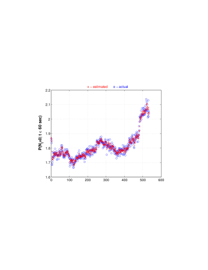
Figure 2: Cox Process with Feller intensity fitted to BRL/USD futures sell orders (ticker DOL FUT - maturity NOV09)

From figure 1 we can see the model flexibility in reacting to different changes in the numbers of orders submitted. In this case, the model seems to fit quite well to actual order flow and the differences between actual and theoretical probability indicate that, on average, the model tends to slightly under-estimate actual occurrence of sell orders. In order to assess the model fitted we conducted a diagnostic checking for possible misspecifications based on the standardized residuals. For a well specified model we need the residuals follows a white noise process.

L	Q(L)	p-value
5	8.36	0.13
10	13.47	0.19
15	17	0.31

Table 2: Ljung-Box test for residual correlation

Table 2 contains the Ljung-Box statistics up to the $15^{th}$ lag. The LB test statistic allows us to not reject, at a high significance level, the hypothesis that errors are white noise. In the absence of dependence in errors the Feller process for intensity seems to be a right choice to describe the observed sell orders behavior.

7 Simulation results

In this section, to analyze the performance of our estimation algorithm we simulate various Cox Process outcomes using a known parameter set and proceed to estimate the model parameters. This simulation exercise is intended to indicate how effective this technique is in terms of identifying parameters. The simulations for the unobservable state variables have been drawn from the noncentral Qui-Square distribution, $f_{\lambda}(d,l)$, and the measurement errors have been simulated as normal random variables with zero means.

The simulation of a sample path for the Cox process with 500 elements, followed by application of the estimation algorithm, is repeated 250 times. The following table summarize the results of the simulation exercise for the Cox Process. The table reports the true values, the mean estimate over the 250 simulations, the Mean Quadratic Error, and the associated standard deviation of the estimates.

	$\theta$	$\kappa$	$\sigma$
Actual Value	0.04	0.2	0.05
Mean estimate	0.04	0.3698	0.0448
MQE	1.5303e-005	0.37	0.0023
Std. Error	0.0039	0.52	0.0001

Table 3: A Analysis of the Kalman Filter estimates by Monte Carlo Simulation

Figure 3: Empirical distribution of $\theta$

Figure 4: Empirical distribution of $\sigma$

Figure 5: Empirical distribution of $\kappa$

8 Final Remarks

Making use of the theoretical framework developed to model interest rate term structure allow us to obtain the Probability Density Function for a Double Stochastic Poisson Process (DSPP) when the intensity process belong to a family of affine diffusion. Furthermore, the stationary distribution for DSSP may be found whenever the intensity process is also stationary. To illustrate our results in this paper one of most common diffusion in interest rate dynamics literature is assumed to drive the intensity process, the one-dimensional Feller process. However the results derived here are valid for any type of affine diffusion in d-dimension.

Finally this paper does not have an empirical focus, and these results are primarily illustrative. The empirical analysis was included to highlight that applied papers on estimating the parameter set for the models examined in section 2 are straightforward.

Appendix A Proof of proposition 16

Specifying the form of $\mu(x,t)$ and $\sigma(x,t)$ into the Theorem 2 we have:

$$\frac{\partial F}{\partial t}+\kappa(\theta-\lambda)\frac{\partial F}{\partial\lambda}+\frac{1}{2}\sigma^{2}\lambda\frac{\partial^{2}F}{\partial\lambda^{2}}-\lambda\mu F=0$$ (58)

With boundary condition $F(T,\lambda,\mu)=1$

Using the results from proposition 3 together with (58):

$$F_{\lambda} =-ABe^{-B\lambda}$$

$$F_{\lambda\lambda} =AB^{2}e^{-B\lambda}$$

$$F_{t} =A_{t}e^{-B\lambda}-AB_{t}\lambda e^{-B\lambda}$$

Plugging the above results into (58):

$$\lambda\left(\frac{\sigma^{2}}{2}AB^{2}-AB_{t}+AB-A\right)=\kappa\theta AB-A_{t}$$ (59)

Since the left hand side is a function of $\lambda$, while the right is independent of it, the following equations must be satisfied:

$$\left\{\begin{array}[]{ccccccccc}\frac{\sigma^{2}}{2}B^{2}&-&B_{t}&+&B&-&1&=&0\\ A_{t}&-&\kappa\theta AB&&&&&=&0\\ \end{array}\right.$$ (60)

The first term of (60) is Riccati equation with solution $B(t,T)=v(t,T)/u(t,T)$ where $v(t,T)$ e $u(t,T)$ are solutions to the following system: :

$$\left\{\begin{array}[]{ccccccc}\frac{\sigma^{2}}{2}v(t,T)&+&u^{{}^{\prime}}(t,T)&&&=&0\\ u(t,T)&+&v^{{}^{\prime}}(t,T)&-&\kappa v(t,T)&=&0\\ \end{array}\right.$$ (61)

Let $\Delta=T-t$, so $\frac{\partial}{\partial t}=-\frac{d}{d\Delta}$ and the system above may be written as:

$$\left\{\begin{array}[]{ccccccc}\frac{\sigma^{2}}{2}v(\Delta)&-&u^{{}^{\prime}}(\Delta)&&&=&0\\ u(\Delta)&-&v^{{}^{\prime}}(\Delta)&-&\kappa v(\Delta)&=&0\\ \end{array}\right.$$ (62)

From the second term of (62) we have:

$$\left\{\begin{array}[]{ccccccc}u(\Delta)&=&&+&v^{{}^{\prime}}(\Delta)&+&\kappa v(\Delta)\\ u^{{}^{\prime}}(\Delta)&=&&+&v^{{}^{\prime\prime}}(\Delta)&+&\kappa v^{{}^{\prime}}(\Delta)\\ \end{array}\right.$$ (63)

Substituting into (62) and rewriting this in terms of $\mathcal{D}$-operators:

$$\left(\mathcal{D}^{2}+\kappa\mathcal{D}-\frac{\sigma^{2}}{2}\right)v(\Delta)=0$$ (64)

Taking the roots of the quadratic equation (65) together with the boundary condition allow write the solution as:

$$v(\Delta)=e^{0.5(\gamma-\kappa)\Delta}-e^{0.5(-\gamma-\kappa)\Delta}$$ (65)

Substituting into (63) gives:

$$u(\Delta)=0.5(\gamma-\kappa)e^{0.5(\gamma-\kappa)\Delta}-0.5(-\gamma+\kappa)e^{0.5(-\gamma-\kappa)\Delta}$$ (66)

Since $\Delta=T-t$, the solution of the Riccati equation is obtained from (65) and (66):

$$B(t,T) =v(\Delta)/u(\Delta)$$

$$B(t,T) =\left[\frac{2\left(e^{-\gamma(T-t)}-1\right)}{\left(\gamma+\kappa\right)\left(e^{-\gamma(T-t)}-1\right)+2\gamma}\right]$$ (67)

Now consider equation (60) with $T$ fixed, so $A(t,T)$ is a function of $t$ only. Hence:

$$\frac{\partial A}{\partial t} =\kappa\theta AB$$

$$A(t,T) =exp\left(-\kappa\theta\int_{t}^{T}B(s,T)ds\right)$$

inserting $B(t,T)$ according to (67) gives:

$$A(t,T)=\frac{2\kappa\theta}{\sigma^{2}}\ln\left(\frac{2\gamma\left(e^{(\gamma+\kappa)/2}\right)}{\left(\gamma+\kappa\right)\left(e^{-\gamma(T-t)}-1\right)+2\gamma}\right)$$ (68)

$\blacksquare$

Appendix B Sketch of the proof of proposition 6

Let $p(s,t,x,y)$ be the transition density of $\{\lambda_{t}:t\in\mathbb{R}_{+}\}$, for simplicity assume that $\lambda_{t}=c\in\mathbb{R}_{+}$ at instant $0$. From the Forward Kolmogorov equation:

$$\frac{\partial p}{\partial t}(t,y)=\frac{1}{2}\frac{\partial^{2}}{\partial y^{2}}\biggl{[}\sigma^{2}(y)p(t,y)\biggr{]}-\frac{\partial}{\partial}\biggl{[}\mu(y)p(t,y)\biggr{]}$$ (69)

The stationary distribution must satisfies $\Psi(y)=\int\Psi(x)p(t,x,y)dx\hskip 8.5359pt\mbox{for all}\hskip 8.5359ptt>0$. When reached the stationary distribution is independent of $t$, so $\frac{\partial p}{\partial t}(t,y)=0$. Combining it together with (69), we have:

$$0=\frac{1}{2}\frac{\partial^{2}}{\partial y^{2}}\biggl{[}\sigma^{2}(y)\Psi(y)\biggr{]}-\frac{\partial}{\partial}\biggl{[}\mu(y)\Psi(y)\biggr{]}$$ (70)

Let $s(y)=\exp\left(-\int_{y}\frac{2\mu(\nu)}{\sigma^{2}(\nu)}d\nu\right)$ be the integrating factor, so integrating (70) twice:

$$\Psi(x) =C_{1}\frac{S(x)}{s(x)\sigma^{2}(x)}+C_{2}\frac{1}{s(x)\sigma^{2}(x)}$$ (71)

$$=m(x)[C_{1}S(x)+C_{2}]$$ (72)

Where: $S(x)=\int_{x}s(y)dy$

The constants $C_{1}$ e $C_{2}$ are determined such that $\Psi(x)$ be a probability density function, so

$$\Psi(x)=\frac{1}{M}\frac{1}{\sigma^{2}(x)s(x)}dx\hskip 11.38092pt\forall\hskip 5.69046ptx\in(l,r)$$

Thus, using the form of $s(x)$ and simplifying we have:

$$\Psi(\lambda)=\beta^{\alpha}\frac{1}{\Gamma(\alpha)}e^{-\beta\lambda}\lambda^{\alpha-1}$$

In short, $\Psi(\lambda)=Gamma(\alpha,\beta)$

References

- Albanese and Lawi (2004) C. Albanese and S. Lawi. Laplace transforms for integrals of markov processes. Markov Processes and Related Fields, 11:677–724, 2004.
- Basu and Dassios (2002) S. Basu and A. Dassios. A cox process with log-normal intensity. Insurance: Mathematics and Economics, 31:297–302, 2002.
- Bouzas et al. (2002) P.R. Bouzas, M.J. Valderrama, and A.M. Aguilera. Forecasting a class of doubly poisson processes. Statistical Papers, 43:507–523, 2002.
- Bouzas et al. (2006) P.R. Bouzas, M.J. Valderrama, and A.M. Aguilera. On the characteristic functional of a doubly stochastic poisson process: Application to a narrow-band process. Applied Mathematical Modelling, 30:1021–1032, 2006.
- Brémaud (1972) P. Brémaud. Point Processes and Queues: Martingale Dynamics. Springer-Verlag, New York, 1972.
- Cont et al. (2010) R. Cont, S. Stoikov, and R. Talreja. A stochastic model for order book dynamics. Operations Research, no Prelo, 2010.
- Cox (1955) D. R. Cox. Some statistical methods connected with series of events. Journal of Royal Statistical Society B, 17:129–164, 1955.
- Cox et al. (1985) J. Cox, J. Ingersoll, and S. Ross. A theory of the term structure of interest rates. Econometrica, 53:385–408, 1985.
- Dai and Singleton (2000) Q. Dai and K. Singleton. Specification analysis of affine term structure models. The Journal of Finance, LV(5):1943–1978, 2000.
- Dalal and McIntosh (1994) S. Dalal and A. McIntosh. When to stop testing for large software systems with changing code. IEEE Trans. Software Eng, 20:318–323, 1994.
- Daley and Vere-Jones (1988) D.J. Daley and D. Vere-Jones. An Introduction to Theory of Point Processes. Springer-Verlag, New York, 1988.
- Dassios and Jang (2008) A. Dassios and J. Jang. The distribution of the interval between events of a cox process with shot noise intensity. Journal of Applied Mathematics and Stochastic Analysis, 2008.
- Duffie et al. (2003) D. Duffie, D. Filipovic, and W. Schachermayer. Affine processes and applications in finance. Annals of Applied Probability, 13:984–1053, 2003.
- Duffie and Kan (1996) D. Duffie and R. Kan. A yield-factor model of interest rates. Mathematical Finance, 6:379–406, 1996.
- Duffie and Singleton (1999) D. Duffie and K. Singleton. Modeling term structures defautable bonds. Review of Financial Studies, 12:687–720, 1999.
- Gail et al. (1980) M. Gail, T. Santner, and C. Brown. An analysis of comparative carcinogenesis experiments based on multiple times to tumor. Biometrics, 36:255–266, 1980.
- Glasserman and Kim (2010) P. Glasserman and K.K. Kim. Moment explosions and stationary distributions in affine diffusion models. Mathematical Finance, 20:1–33, 2010.
- Grandell (1976) J. Grandell. Doubly Stochastic Process. Springer-Verlan, New York, edition, 1976.
- Harvey (1989) A.C. Harvey. Forecasting, structural time series models and the Kalman Filter. Cambridge University Press, Cambridge, 1989.
- Kallenberg (1986) O. Kallenberg. Random Measures. Academic Press, London, edition, 1986.
- Karatzas and Shreve (1991) I. Karatzas and S. Shreve. Brownian Motion and Stochastic Calculus. Springer-Verlan, New York, edition, 1991.
- Karlin and Taylor (1981) S. Karlin and H. Taylor. A Second Course in Stochastic Process. Academic Press, New York, 1981.
- Kozachenko and Pogorilyak (2008) Yu. V. Kozachenko and O. O. Pogorilyak. A method of modelling log gaussian cox process. Theory of Probability and Mathematical Statistics, 77:91–105, 2008.
- Lando (1998) D. Lando. On cox processes and credit risky securities. Review of Derivatives Research, 2:99–120, 1998.
- Pinsky (1995) R. Pinsky. Positive Harmonic Functions and Diffusions. Cambridge University Press, 1995.
- Wei et al. (2002) G. Wei, P. Clifford, and J. Feng. Population death sequences and cox processes driven by interacting feller diffusions. Journal of Physics A: Mathematical and General, 35:9–31, 2002.