Spectrum of Andreev bound states in Josepshon junctions with a ferromagnetic insulator

Abstract

Ferromagnetic-insulator (FI) based Josephson junctions are promising candidates for a coherent superconducting quantum bit as well as a classical superconducting logic circuit. Recently the appearance of an intriguing atomic-scale 0-$\pi$ transition has been theoretically predicted. In order to uncover the mechanism of this phenomena, we numerically calculate the spectrum of Andreev bound states in a FI barrier by diagonalizing the Bogoliubov-de Gennes equation. We show that Andreev spectrum drastically depends on the parity of the FI-layer number $L$ and accordingly the $\pi$ (0) state is always more stable than the 0 ($\pi$) state if $L$ is odd (even).

, , , ,

1 Introduction

The peculiarity of the proximity effect in superconductor/ferromagnetic-metal (S/FM) bilayers is the damped oscillation of the pair amplitude inside a FM [1, 2]. This anomalous proximity effect leads to the $\pi$ Josephson S/FM/S junction [3, 4] which has the opposite sign to the superconducting order parameter in two S electrodes in the ground state. Experimentally $\pi$-junction was firstly observed by Ryazanov [5] and Kontos [6] and since then a lot of progress has been made in the physics of $\pi$-junctions and now they are proving to be promising elements of superconducting classical and quantum circuits [7, 8, 9, 10].

On the other hands, recently a possibility of $\pi$ junction formation in a Josephson junction with a $ferromagnetic$ $insulator$ (FI) has been theoretically predicted [11, 12, 13, 14, 15, 16, 17, 18, 19, 20]. The $\pi$ junction using such an insulating barrier is very promising for future qubit [21, 22, 23, 24] and microwave [25] applications because of the low decoherence nature [26, 27]. More importantly, it has been shown that the ground state of S/FI/S junction alternates between 0- and $\pi$-states when thickness of FI is increasing by a single atomic layer [16, 18]. In this paper in order to understand the physical mechanism of the anomalous atomic scale 0-$\pi$ transition, we will calculate the spectrum of the Andreev bound states in such systems. Based on this calculation, we will show that Andreev spectrum drastically depends on the parity of the FI layer number $L$ and thence the $\pi$ (0) state is always more stable than the 0 ($\pi$) state if $L$ is odd (even).

In this paper we focused on the one dimensional $s$-wave junction with a FI barrier (Fig. 1(a)). It should be noted that the qualitatively same result can be obtained for two- or three-dimensional cases.

2 Model

Figure 1: (a) The Josephson junction with a ferromagnetic-insulator barrier on the one-dimensional tight-binding lattice and (b) transport through Andreev bound states. An electron (black circle) is reflected as a hole (white circle) at the interface with the left superconductor and the hole is reflected back as an electron on the right interface. The net result is a Cooper pair transfer through the junction.

Let us consider a one-dimensional tight-binding lattice of a superconductor/ferromagnetic-insulator /superconductor (S/FI/S) Josephson junction with $L$ being the thickness or the numbers of the FI lattice sites as shown in Fig. 1(a). The lattice constant is set to be unity. Electronic states in a $s$-wave superconductor are described by the mean-field BCS Hamiltonian,

$$H_{\mathrm{S}} = -t\sum_{n,n^{\prime}\in\mathrm{S},\sigma}c_{n\sigma}^{\dagger}c_{n^{\prime}\sigma}+(2t-\mu_{s})\sum_{n\in\mathrm{S},\sigma}c_{n\sigma}^{\dagger}c_{n\sigma}$$ (1)

$$+ \frac{\Delta}{2}\sum_{n\in\mathrm{S}}\left(c_{n\uparrow}^{\dagger}c_{n\downarrow}^{\dagger}+c_{n\uparrow}^{\dagger}c_{n\downarrow}^{\dagger}+\mathrm{h.c.}\right).$$

Here $c_{n\sigma}^{\dagger}$ ($c_{n\sigma}$) is the creation (annihilation) operator of an electron at a site $n\in\mathrm{S}$ with spin $\sigma=$ ( $\uparrow$ or $\downarrow$ ) and $\mu_{s}$ is the chemical potential. The hopping integral $t$ is considered among nearest neighbor sites and $\Delta$ is the amplitude of $s$-wave pair potential.

The energy dispersion in the Bogoliubov-de Gennes picture and the spin resolved density of states (DOS) for typical FIs are shown schematically in Fig. 2. Experimental studies as well as a first principle calculations indicate that the band structure of an oxide ferromagnet La₄Ba₂Cu₂O₁₀ (La422) [28, 29, 30] and K₂CuF₄ [31, 32, 33] can be described by Fig. 2(b) in which the up- and down-spin bands are located below and above the Fermi energy respectively. The exchange splitting $V_{\mathrm{ex}}$ of La422 is numerically estimated to be 0.34 eV. Since the exchange splitting is large and the bands are originally half-filled, La422 becomes FI with a Curie temperature of 5 K [28]. Another possible candidates for the FI barrier are spinels [34, 35], e.g., NiFe₂O₄, rare-earth monopnictides [36, 37, 38, 39], e.g., GdN, and Yttrium iron garnet (Y₃Fe₅O₁₂) [40, 41].

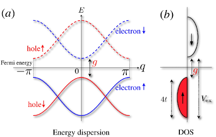
Figure 2: (a)The band structure of a ferromagnetic-insulator in the Bogoliubov-de Gennes picture and (b) corresponding spin-resolved density of states (DOS). The energy dispersion for a hole with spin $\sigma$ is obtained as a mirror image of that for an electron with spin $\sigma$ with respect to Fermi energy.

The Hamiltonian of a ferromagnetic layer can be described by a single-band tight-binding model [20] as

$$H_{\mathrm{FI}} = -t\sum_{n,n^{\prime}\in\mathrm{F},\sigma}c_{n\sigma}^{\dagger}c_{n^{\prime}\sigma}$$ (2)

$$- \sum_{n\in\mathrm{F}}\left(4t-\mu+\frac{V_{\mathrm{ex}}}{2}\right)c_{n\uparrow}^{\dagger}c_{n\uparrow}$$

$$+ \sum_{n\in\mathrm{F}}\left(4t-\mu+\frac{V_{\mathrm{ex}}}{2}\right)c_{n\downarrow}^{\dagger}c_{n\downarrow},$$

where

$$V_{\mathrm{ex}}=4t+g$$ (3)

is the exchange splitting ($g$ is the gap between up and down spin bands) and $\mu$ is the chemical potential (see Fig. 2(a)). If $V_{\mathrm{ex}}>4t$, this Hamiltonian describes FI as shown in Fig. 2.

3 Andreev bound states and Josephson current

The Hamiltonian can be diagonalized by the Bogoliubov transformation. Due to the the Andreev reflection at S/FI interfaces, the Andreev bound state is formed in the FI barrier (see Fig. 1(b)). Wave functions of the Andreev bound state decay far from the S/FI interface. In what follows, we focus on the subspace for spin-$\uparrow$ electron and spin-$\downarrow$ hole. In superconductors, the wave function of a bound state is given by

$$\Psi_{L}(n)= \Phi_{L}\left[\left(\begin{array}[]{c}u\\ v\end{array}\right)Ae^{-ikn}+\left(\begin{array}[]{c}v\\ u\end{array}\right)Be^{ik^{*}n}\right],$$ (8)

$$\Psi_{R}(n)= \Phi_{R}\left[\left(\begin{array}[]{c}u\\ v\end{array}\right)Ce^{ikn}+\left(\begin{array}[]{c}v\\ u\end{array}\right)De^{-ik^{*}n}\right].$$ (13)

Here $A,B,C$ and $D$ are amplitudes of the wave function for an outgoing quasiparticle, $\phi_{\nu}$ is the phase of a superconductor,

$$\Phi_{\nu} = \mathrm{diag}\left(e^{i\phi_{\nu}/2},e^{-i\phi_{\nu}/2}\right),$$ (14)

with $\nu=L$ ($R$) indicates an left (right) superconductor, and

$$u = \sqrt{\frac{1}{2}\left(1+\frac{\Omega}{E}\right)}$$ (15)

$$v = \sqrt{\frac{1}{2}\left(1-\frac{\Omega}{E}\right)},$$ (16)

with

$$\Omega=\sqrt{E^{2}-\Delta^{2}}.$$ (17)

The energy $E$ is measured from the Fermi energy and

$$k=\frac{\pi}{2}+i\cosh^{-1}\sqrt{1+\frac{\Delta^{2}-E^{2}}{4t^{2}}}$$ (18)

is the complex wave number. In a FI, the wave function is given by

$$\Psi_{\mathrm{FI}}(n) = \left(\begin{array}[]{c}f_{1}e^{-iq_{e}n}\\ g_{1}e^{-iq_{h}n}\end{array}\right)+\left(\begin{array}[]{c}f_{2}e^{iq_{e}n}\\ g_{2}e^{iq_{h}n}\end{array}\right),$$ (23)

with

$$q_{e} = \pi+i\cosh^{-1}\left(1+\frac{E}{2t}+\frac{g}{4t}\right),$$ (24)

$$q_{h} = i\cosh^{-1}\left(1+\frac{E}{2t}+\frac{g}{4t}\right),$$ (25)

and $f_{1},f_{2},g_{1}$ and $g_{2}$ are amplitudes of wave function in a FI.

By applying the boundary conditions,

$$\Psi_{L}(0) = \Psi_{\mathrm{FI}}(0),$$ (26)

$$\Psi_{L}(1) = \Psi_{\mathrm{FI}}(1),$$ (27)

$$\Psi_{R}(L) = \Psi_{\mathrm{FI}}(L),$$ (28)

$$\Psi_{R}(L+1) = \Psi_{\mathrm{FI}}(L+1),$$ (29)

we can obtain a secular equation for amplitudes $A$, $B$, $C$ and $D$. From this equation, we can numerically calculate the Andreev levels $\varepsilon_{j}$ as a function of the phase difference $\phi=\phi_{L}-\phi_{R}$, where $j=1,\cdots,4$.

The Josephson current can be calculated from the Beenakker formula [42], $i.e.,$

$$I_{J}(\phi)=\frac{2e}{\hbar}\sum_{j}\frac{\partial\varepsilon_{j}(\phi)}{\partial\phi}f\left[\varepsilon_{j}(\phi)\right],$$ (30)

where $f\left(\varepsilon\right)$ is the Fermi-Dirac distribution function. In the case of a high barrier limit, the Josephson current phase relation is described by

$$I_{J}(\phi)=I_{C}\sin\phi.$$ (31)

Thus we define the Josephson critical current $I_{C}$ as

$$I_{C}=I_{J}\left(\frac{\pi}{2}\right).$$ (32)

If $I_{C}$ is negative (positive), then the $\pi$ (0) junction is realized.

4 Numerical results

In this section, we show numerical results for the spectrum of Andreev bound states for a conventional S/I/S junction and an S/FI/S junction. In the calculation, we set $\mu=\mu_{s}=2t$, and $\Delta=0.01t$.

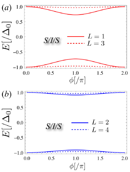
Figure 3: The Andreev spectrum in an S/I/S Josephson junction for the case of (a) odd and (b) even insulating-layer number $L$. In the calculation, we set $g=0.25t$, $\mu=\mu_{s}=2t$, and $\Delta=0.01t$.

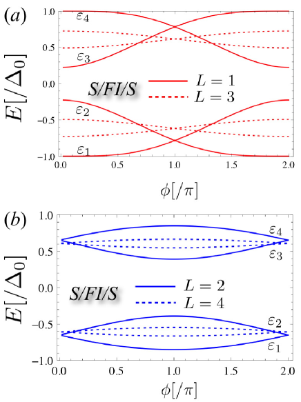
Figure 4: The Andreev spectrum in an S/FI/S Josephson junction for the case of (a) odd and (b) even FI-layer number $L$. In the calculation, we set $g=t$, $\mu=\mu_{s}=2t$, and $\Delta=0.01t$.

Let us firstly consider Andreev bound states in an S/I/S junction. Fig. 3 shows the Andreev spectrum as a function of the thickness of the insulating barrier $L$. Due to the spin degeneracy, we have 2 Andreev levels for a given $\phi$ and $L$. It is evident that the energy minimum is at $\phi=0$ irrespective of the value of $L$. So the overall feature of Andreev levels does not depend on $L$. On the other hand, Fig. 4 shows the $L$ dependence of the Andreev spectrum for an S/FI/S junction. The results indicate that the overall feature of the spectrum strongly depends on the parity of $L$ and show that the energy minimum of $\varepsilon_{1}$ for odd $L$ is at $\phi=0$, whereas for even $L$ at $\phi=\pi$.

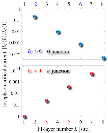
Figure 5: Josephson critical current $I_{C}$ at $T=0.01T_{c}\ll T_{c}$ as a function of the FI layer thickness $L$ for $g=t$. The red (blue) circles indicate the $\pi$(0) junction.

In Fig. 5, we show the Josephson critical current for an S/FI/S junction as a function of $L$. Temperature $T$ is set to be $0.01T_{c}\ll T_{c}$, where $T_{c}$ is the transition temperature of a superconductor. The $\pi$(0)-state is always more stable than the 0($\pi$)-state when the thickness of FI is an odd(even) integer. Based on the Andreev spectrum (Fig. 4) the reason can be explained as follows. At low temperatures, only the Andreev levels below the Fermi energy i.e., $\varepsilon_{1}$ and $\varepsilon_{2}$, contribute to $I_{C}$. In the odd (even) $L$ cases, the $\pi$- (0-) junction is stable because of

$$\left.\frac{\partial\varepsilon_{1}(\phi)}{\partial\phi}\right|_{\phi=\pi/2} > (<)0,$$ (33)

$$\left.\frac{\partial\varepsilon_{2}(\phi)}{\partial\phi}\right|_{\phi=\pi/2} < (>)0,$$ (34)

$$\left|\frac{\partial\varepsilon_{2}(\phi)}{\partial\phi}\right|_{\phi=\pi/2} > \left|\frac{\partial\varepsilon_{1}(\phi)}{\partial\phi}\right|_{\phi=\pi/2}.$$ (35)

Above analysis provides an new physical interpretation of the atomic scale 0-$\pi$ transition from the view point of the Andreev spectrum.

5 Summary

To summarize, we have theoretically studied the Andreev levels and the Josephson current in S/FI/S junctions by solving the Bogolubov-de Gennes equation in order to understand the physical mechanism of the atomic scale 0-$\pi$ transition. A characteristic and important feature for such systems is that the Andreev spectrum strongly depends on the parity of the thickness of the FI layer $L$. As a result, the junctions show the atomic scale 0-$\pi$ transition. Our finding suggests a way of understanding the physical origin of the atomic scale 0-$\pi$ transition in ferromagnetic-insulator based Josephson junctions. In this paper, we have only considered the Josephson transport in the low temperature regime, i.e., $T\ll T_{c}$. The calculation of $I_{C}$ in the finite temperature region and the analysis based on the Andreev spectrum (Fig. 4) are important future problems.

References

- [1] L. N. Bulaevskii, V. V. Kuzii, A. A. Sobyanin, JETP Lett. 25 (1977) 291.
- [2] A. I. Buzdin, L. N. Bulaevskii, S. V. Panyukov, JETP Lett. 35 (1982) 179.
- [3] A. A. Golubov, M. Y. Kupriyanov, E. Il’ichev, Rev. Mod. Phys. 76 (2004) 411.
- [4] A. I. Buzdin, Rev. Mod. Phys. 77 (2005) 935.
- [5] V. V. Ryazanov, V. A. Oboznov, A. Y. Rusanov, A. V. Veretennikov, A. A. Golubov, J. Aarts, Phys. Rev. Lett. 86 (2001) 2427.
- [6] T. Kontos, M. Aprili, J. Lesueur, F. Genêt, B. Stephanidis, R. Boursier, Phys. Rev. Lett. 89 (2002)137007.
- [7] L.B. Ioffe, V.B. Geshkenbein, M.V. Feigelman, A.L. Fauchere, G. Blatter, Nature 398 (1999) 679.
- [8] I. Petkovic, M. Aprili, Phys. Rev. Lett. 102 (2009)157003.
- [9] V. M. Krasnov, T. Golod, T. Bauch, and P. Delsing, Phys. Rev. B 76 (2007) 224517.
- [10] A. K. Feofanov, V. A. Oboznov, V. V. Bolginov, J. Lisenfeld, S. Poletto, V. V. Ryazanov, A. N. Rossolenko, M. Khabipov, D. Balashov, A. B. Zorin, P. N. Dmitriev, V. P. Koshelets, A. V. Ustinov, Nature Phys. 6 (2010) 593.
- [11] Y. Tanaka, S. Kashiwaya, Physica C 274 (1997) 357.
- [12] J. C. Cuevas, M. Fogelström, Phys. Rev. B 64 (2001) 104502.
- [13] E. Zhao, T. Löfwander, and J. A. Sauls Phys. Rev. B 70 (2004) 134510.
- [14] S. Kawabata, Y. Asano, Int. J. Mod. Phys. B 23 (2009) 4329.
- [15] S. Kawabata, Y. Asano, Y. Tanaka, S. Kashiwaya, Physica C 469 (2009) 1621.
- [16] S. Kawabata, Y. Asano, Y. Tanaka, A. A. Golubov, S. Kashiwaya, Phys. Rev. Lett. 104 (2010) 117002.
- [17] S. Kawabata, Y. Asano, Y. Tanaka, S. Kashiwaya, Physica E 42 (2010) 1010.
- [18] S. Kawabata, Y. Asano, Low Temp. Phys. 36 (2010) 915.
- [19] S. Kawabata, Y. Asano, Y. Tanaka, A. A. Golubov, S. Kashiwaya, Physica C 470 (2010) 1496.
- [20] S. Kawabata, Y. Tanaka, Y. Asano, Physica E 43 (2011) 722.
- [21] S. Kawabata, S. Kashiwaya, Y. Asano, Y. Tanaka, Physica C 437-438 (2006) 136.
- [22] S. Kawabata, S. Kashiwaya, Y. Asano, Y. Tanaka, A. A. Golubov, Phys. Rev. B 74 (2006) 180502(R).
- [23] S. Kawabata, A. A. Golubov, Physica E 40 (2007) 386.
- [24] S. Kawabata, Y. Asano, Y. Tanaka, S. Kashiwaya, A. A. Golubov, Physica C 468 (2008) 701.
- [25] S. Hikino, M. Mori, S. Takahashi, and S. Maekawa, J. Phys. Soc. Jpn. 80 (2011) 074707.
- [26] G. Schön, A. D. Zaikin, Phys. Reports 198 (1990) 237.
- [27] T. Kato, A. A. Golubov, Y. Nakamura, Phys. Rev. B 76 (2007) 172502.
- [28] F. Mizuno, H. Masuda, I. Hirabayashi, S. Tanaka, M. Hasegawa, U. Mizutani, Nature 345 (1990) 788.
- [29] V. Eyert, K. H. Höc, P. S. Riseborough, Europhys. Lett. 31 (1995) 385.
- [30] W. Ku, H. Rosner, W. E. Pickett, R. T. Scalettar, Phys. Rev. Lett. 89 (2002) 167204.
- [31] I. Yamada, J. Phys. Soc. Jpn. 33 (1972) 979.
- [32] K. Hirakawa, H. Ikeda, J. Phys. Soc. Jpn. 35 (1973) 1328.
- [33] V. Eyert, K. H. Höc, J. Phys.: Condens. Matter 5 (1993) 2987.
- [34] Z Szotek, W. M. Temmerman, A. Svane, L. Petit, P. Strange, G. M. Stocks, D. Ködderitzsch, W. Hergert, H. Winter, J. Phys.: Condens. Matter 16 (2004) S5587.
- [35] Z. Szotek, W. M. Temmerman, D. Ködderitzsch, A. Svane, L. Petit, H. Winter, Phys. Rev. B 74 (2006) 174431.
- [36] C-G. Duan, R. F. Sabirianov, W. N. Mei, P. A. Dowben, S. S. Jaswal, E. Y. Tsymbal, J. Phys.: Condens. Matter 19 (2007) 315220.
- [37] P. Larson, W. R. L. Lambrecht, A. Chantis, M. van Schilfgaarde Phys. Rev. B 75 (2007) 045114.
- [38] A. R. H. Preston, B. J. Ruck, W. R. L. Lambrecht, L. F. J. Piper, J. E. Downes, K. E. Smith, H. J. Trodahl, App. Phys. Lett. 96 (2010) 032101.
- [39] H. M. Liu, C. Y. Ma, C. Zhu, J-M. Liu, J. Phys.: Condens. Matter 23 (2011) 245901.
- [40] W. Y. Ching, Z-Q Gu, and Y-N. Xu, J. App. Phys. 89 (2001) 6883.
- [41] X. Jia, K. Liu, K. Xia, G. E. W. Bauer, arXiv:1103.3764 (2011).
- [42] C. W. J. Beenakker, Phys. Rev. Lett. 67 (1991) 3836.