Wavefront sensing with a brightest pixel selection algorithm

Abstract

Astronomical adaptive optics systems with open-loop deformable mirror control have recently come on-line. In these systems, the deformable mirror surface is not included in the wavefront sensor paths, and so changes made to the deformable mirror are not fed back to the wavefront sensors. This gives rise to all sorts of linearity and control issues mainly centred on one question: Has the mirror taken the shape requested? Non-linearities in wavefront measurement and in the deformable mirror shape can lead to significant deviations in mirror shape from the requested shape. Here, wavefront sensor measurements made using a brightest pixel selection method are discussed along with the implications that this has for open-loop AO systems. Discussion includes elongated laser guide star spots and also computational efficiency.

Keywords: Adaptive Optics

1 Introduction

Adaptive optics (AO) is a widely used technology on large near infra-red and optical telescopes, and almost all current and planned facility class science telescopes will have an AO system. AO systems have been used to obtain a large number of science results that would otherwise have been impossible due to atmospheric induced perturbations(2004A&A...417L..21G; 2005ApJ...625.1004M). Novel applications for AO such as high resolution imaging over a wide-field are currently being studied and implemented(2004SPIE.5490..236Mshort), for example multi-object AO (MOAO) (canaryresultsshort).

Starlight passing through the Earth’s atmosphere is distorted by the introduction of random perturbations due to time-varying refractive index changes in the atmosphere(tatarski). This means that forming a diffraction limited image is no longer possible, and the effective resolution of a telescope is reduced. However, corrective measures can be taken, which by changing the shape of a deformable mirror (DM) in response to a wavefront sensor (WFS) can greatly reduce the impact of the atmospheric turbulence (roddier). An AO system, used to perform this task, is composed of WFSs and DMs.

Traditional AO systems use a WFS to view the incident wavefront after correction by the DM has been applied, meaning that only partial further correction is then required in the resulting closed-loop system. However, recent progress has been made with open-loop systems (canaryresultsshort) such as those required by MOAO. In these systems, the wavefront sensors are not sensitive to the corrections applied to the DM, but rather measure the perturbed wavefront directly. These measurements are then used to control the DM without subsequent direct measurement of whether the desired control shape has been realised (so called open-loop control), reducing the impact of atmospheric turbulence for the science path only, but not for the WFSs. In such open-loop systems, the characteristics of the DM and WFSs must be well known, as any non-linearities will result in the wrong correction being applied to the DM. It is therefore desirable that any processing algorithm used should be linear.

A Shack-Hartmann wavefront sensor consists of an array of lenses, each of which effectively samples part of the telescope pupil plane. The local tilt of a wavefront across each lenslet is measured by determining the position of the spot produced by the lenslet on the detector; if there is no tilt, the spot on the detector will appear in a position corresponding to the centre of the sub-aperture. The standard way of determining the spot position, which is used in almost all Shack-Hartmann based astronomical AO systems used on-sky, is by using a centre of gravity algorithm (2006MNRAS.371..323T). However this is sensitive to noise (background, readout and photon arrival statistics) and can perform poorly for open-loop systems.

Correct image calibration (including removal of background light and detector dark noise, application of a flat field map and thresholding) is very difficult to achieve, as the necessary calibration maps may be time and temperature dependent. Incorrect calibration leads to incorrect wavefront estimation and hence to incorrect correction with a DM, which for open-loop systems can lead to significant performance loss. This is less of a problem for closed-loop systems because spot motions are usually small and less affected by these systematic errors as static aberrations can be corrected using WFS offsets (reference measurements). However incorrect calibration may lead to incorrect WFS offsets, giving rise to non-common path wavefront error. Detector noise, and noise due to the random stochastic nature of photon arrival times will also impact wavefront estimation accuracy. For typical AO system working regimes using faint fluxes, this is a significant source of noise.

Further, when a laser guide star (LGS) is used, the shape of Shack-Hartmann spots changes across the wavefront sensor, taking an elongated shape in sub-apertures away from the LGS launch position due to system geometry. A conventional flat threshold is then no longer ideal (2009MNRAS.398.1461L) and using a non-constant threshold can be of advantage.

In this paper, a brightest pixel selection algorithm is investigated which can improve wavefront slope estimation accuracy by applying a different threshold value on a per-sub-aperture basis, and hence improve AO system performance. This algorithm has previously been proposed (by author E. Gendron) but never formally published or studied, and here we report on the first real-time implementation of it, and investigate linearity and how to best apply this algorithm in different conditions and situations. This algorithm is primarily suited to Shack-Hartmann systems with at least $4\times 4$ pixels per sub-aperture.

If §2 the brightest pixel selection algorithm is described, in §3 performance measurements and comparisons are given, and in §4 conclusions are made.

2 The brightest pixel selection algorithm

The brightest pixel algorithm as defined in this paper is simple: Select the brightest $N$ pixels within a given Shack-Hartmann sub-aperture, and set all other pixel values to zero. This modified sub-aperture is then processed in the standard way to compute wavefront slope, for example using a centre of gravity algorithm to measure the spot position thus obtaining the wavefront slope across the sub-aperture. This algorithm benefits from the removal of pixels that contain noise only and not useful signal, and is less sensitive to random noise than the radial thresholding technique proposed by (2009MNRAS.398.1461L) which sets a threshold at a fraction of the brightest pixel in a sub-aperture. To be valuable for open-loop AO systems, the linearity and performance of the brightest pixel selection algorithm must be investigated.

A modified version of the brightest pixel selection algorithm is also possible, and includes subtraction of the value of the $N+1^{th}$ brightest pixel in a given sub-aperture from all pixels in the sub-aperture, after which all negative values are set to zero. In this paper, the performance of both of these algorithms is investigated. Fig. 1 demonstrates these algorithms.

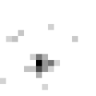
Figure 1: A figure demonstrating brightest pixel selection algorithm for a single Shack-Hartmann sub-aperture spot with (from left to right) no selection, after selection of the brightest 20 pixels (setting all others to zero), and after selection of brightest 20 pixels and subtraction of 21${}^{\textrm{st}}$ brightest pixel, setting negative values to zero. A linear scale has been used and each image has been normalised with pixel values ranging from 0 to 1.

2.1 Application of brightest pixel selection

The brightest pixel selection algorithm has been used on-sky with the CANARY (canaryshort) AO test-bench system on the William Herschel Telescope (WHT) in September and November 2010. For this purpose, the algorithm had been integrated with the the Durham AO real-time controller (DARC) real-time control system (RTCS) (basden9). However the operation of this algorithm had not been studied in depth and so the number of pixels selected was somewhat arbitrary, usually around 15. In this paper, an in-depth study of the performance of this algorithm is made, allowing more educated determination of the number of pixels to select when used in future, for example during the future phases of CANARY in 2011–2015.

The implementation of this algorithm in the real-time control system is fairly straightforward, though must be efficient so that system latencies are not significantly increased, which would lead to performance degradation. It is carried out as follows on a sub-aperture by sub-aperture basis.

1. A quick-sort algorithm is used to sort all the pixels of a given sub-aperture.

2. The $n^{th}$ brightest pixel is selected as the threshold value (the first pixel being the brightest).

3. The $n+1^{th}$ brightest pixel is selected as an optional offset (bias) value.

4. The sub-aperture pixels with intensity below the threshold value are set to zero.

5. Optionally, pixels with intensity equal to or greater than the threshold value have the offset (bias) value subtracted. We hereafter term the version of this algorithm which includes this subtraction the “$N+1^{th}$ subtracted algorithm”.

6. Shack-Hartmann slope measurement then proceeds in a standard way (e.g. weighted centre of gravity, correlation, etc).

Sorting the pixels in each sub-aperture is computationally expensive, particularly for systems with larger numbers of pixels per sub-aperture. CANARY has 256 pixels per natural guide star (NGS) sub-aperture, though fortunately, the RTCS used is powerful enough to handle these extra calculations without adding significant latency. In section 3.9 the computational complexity of the brightest pixel selection algorithm is explored.

2.2 Performance criteria

The performance of the pixel selection algorithm has been investigated using Monte-Carlo simulation of an open-loop Shack-Hartmann wavefront sensor (i.e., viewing the atmospheric turbulence only, not a deformable mirror) following (basden5). The slope measurements computed when using the brightest pixel selection algorithm are compared with slope measurements computed using a noiseless image without the brightest pixel selection algorithm (giving the best Shack-Hartmann estimation of the true slope measurement), and the root-mean-square (RMS) error of many thousands of such comparisons is computed. For each comparison a different realisation of atmospheric turbulence is used. In this paper, the performance criteria is therefore defined by

$$R=\sqrt{\frac{\sum_{m=1}^{N}\left(S_{\textrm{true}}(m)-S_{\textrm{estimated}}(m)\right)^{2}}{N}}$$ (1)

where $N$ is the number of measurements taken and $S(m)$ is the $m^{th}$ individual slope measurement measured with $m^{th}$ atmospheric turbulence realisation computed with either no pixel selection and no noise (true), or with brightest pixel selection (estimated). A lower value of $R$ means more accurate estimation of the local wavefront slope, i.e. better performance. It should be noted that this RMS performance criteria does not contain bias, but is due solely to the noise introduced (photon shot noise and readout noise). The following operations are performed:

1. A realisation of the optical wavefront phase introduced by atmospheric perturbations is produced.

2. A WFS is modelled producing a Shack-Hartmann spot pattern with photon noise and readout noise added.

3. Image calibration including brightest pixel selection is performed.

4. A centre of gravity algorithm is used to estimate wavefront slope for each sub-aperture.

5. The estimated wavefront slope is compared with the slope calculated using a noiseless Shack-Hartmann image (no read noise or photon shot noise).

6. The process is repeated many times computing the RMS difference between estimated and true wavefront slopes.

It should be noted that we are comparing measurements with a noiseless Shack-Hartmann image rather than the true slope measurement. This is intentional, because it allows us to investigate the best possible way of processing Shack-Hartmann data using the brightest pixel selection algorithm, rather than comparing how well this performs relative to a perfect wavefront sensor (which a noiseless Shack-Hartmann is not). For reference purposes, Fig. 2 shows the deviation (bias) of perfect Shack-Hartmann measurements from true wavefront slope.

Figure 2: A figure showing the bias in wavefront slope measurement by a noiseless Shack-Hartmann wavefront sensor. The wavefront sensor here used $16\times 16$ pixels per sub-aperture. This bias is due to the pixellated and truncated nature of a Shack-Hartmann sensor.

In our simulations, detectors are modelled with a uniform response, and so a flat field image of unity is used. We do not add any detector dark noise (it can be minimised at the typical frame rates that astronomical wavefront sensors are operated at) and so no bias subtraction is necessary. A detector background of 50 counts is added (unless otherwise stated), and a background subtraction of 50 counts is removed. It should be noted that we do not subtract at a level of $3\sigma$ above detector noise because this adds a bias in slope estimation.

2.3 Model description

In this paper, results are concentrated on a model based on the CANARY MOAO demonstrator instrument because that is where the brightest pixel selection algorithm has been used on-sky. A telescope with a 4.2 m diameter primary mirror and an AO system with WFSs having $7\times 7$ sub-apertures is used with a detection wavelength of 640 nm.

The baseline configuration for these comparisons comprises a signal level of 200 photons per sub-aperture and a RMS readout noise of 2 photo-electrons. Each sub-aperture consists of $16\times 16$ pixels with a pixel scale of 0.22 arcsec per pixel. The atmosphere is modelled with Von Karman statistics with an outer scale of 30 m and a Fried’s parameter ($r_{0}$) of 12.5 cm (at 500 nm, representing fairly average atmospheric statistics) corresponding to $d/r_{0}=4.8$ where $d$ is the effective sub-aperture diameter (the telescope pupil diameter divided by the number of sub-apertures across it). The Shack-Hartmann spots are modelled as having an Airy disc point spread function (PSF) with a diameter (to first minimum) of 0.7 arcsec (20% of a sub-aperture). A rough estimate for signal-to-noise ratio can be made by considering photon and readout noise, giving a value of about 6 following

$$\mathrm{SNR}=\frac{n_{\mathrm{ph}}}{\sqrt{n_{\mathrm{ph}}+\sigma_{e}^{2}N_{\mathrm{pix}}}}$$ (2)

where $n_{\mathrm{ph}}$ is the number of photons per sub-aperture per frame, $\sigma_{e}$ is the detector read noise, and $N_{\mathrm{pix}}$ is the number of pixels per sub-aperture.

2.4 Linearity

As mentioned previously, for open-loop AO systems, linearity is important for achieving good correction. The linearity of the brightest pixel selection algorithm has been studied by placing known, gradually increasing, tilts across a sub-aperture, and comparing the measured slope using all pixels and with brightest pixel selection. In both cases, the WFS is noiseless, with no readout noise or photon arrival statistics added. In an ideal case, with a linear WFS, the measured slope will be directly proportional to the true slope.

3 Results

A parameter space including the number of brightest pixels selected, WFS readout noise, signal level, background level errors and atmospheric model details has been explored to find the optimum number of brightest pixels to use for selection, and results are presented here.

For each of these results, extrapolation to using the 256 brightest pixels (all pixels) will give the performance that would be achieved using all available pixels (the traditional approach), though this is not explicitly shown to simplify the data and make the results clearer.

3.1 Sensitivity to Shack-Hartmann PSF size

The size of a Shack-Hartmann generated spot will depend on the wavefront sensor pixel scale used and on the optical aberrations introduced by the lenslet array and optics, as well as the seeing conditions. If light is concentrated into only a few pixels then intuitively, using fewer brightest pixels is likely to give better performance since fewer pixels will actually contain signal. Fig. 3(a) shows the spot PSFs used in these comparisons and Fig. 3(b) shows the same spots after broadening due to atmospheric perturbation. Fig. 3(c) shows the slope calculation accuracy as a function of number of brightest pixels used for different Shack-Hartmann spot diameters (with lower results representing greater accuracy). It can be seen that smaller spot sizes favour a lower number of brightest pixels used, but that this trend is not as pronounced as might be expected from the relative unbroadened PSF spot sizes. However, since the atmosphere broadens these PSFs as shown in Fig. 3(b), they then appear more similar in size. It can be seen that background subtraction of the next brightest pixel value (using the “$N+1^{th}$ subtracted algorithm”) is advantageous. We find that this is in general the case (as expected from linearity considerations), and so the rest of the results presented in this paper show cases using the “$N+1^{th}$ subtracted algorithm” only, unless there is good reason to also show results corresponding to no subtraction. This plot suggests that at least the 20 brightest pixels should be used along with subtraction of the 21${}^{\textrm{st}}$ brightest pixel. By extrapolating the curves to 256 brightest pixels, the slope estimation accuracy of the conventional case (with no brightest pixel selection) can be seen to be significantly poorer than using brightest pixel selection.

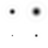
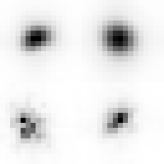
(a) (b) (c)

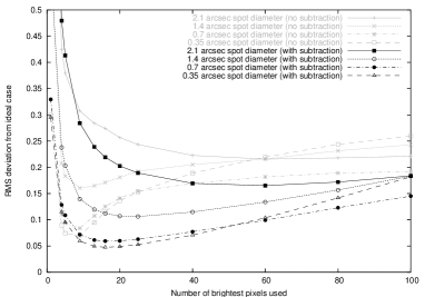
Figure 3: (a) A diagram showing the Shack-Hartmann point spread functions used for comparison of the brightest pixel selection algorithm. The spots have Airy diameters equal to 0.35, 0.7, 1.4 and 2.1 arcsec respectively from small to large (corresponding to radii of 5%, 10%, 20% and 30% of the sub-aperture), normalised to the same maximum brightest pixel value for display purposes. (b) A diagram showing an example of atmospheric broadened Shack-Hartmann point spread functions for comparison with (a). (c) A plot showing slope calculation accuracy (lower is better) as a function of number of brightest pixels used for different spot radii. Comparisons for pixel selection only (labelled “no subtraction”), and using the “$N+1^{th}$ subtracted algorithm” (labelled “with subtraction”) are made. Detector readout noise and photon shot noise have been included.

3.2 Sensitivity to signal level

The signal level received by the wavefront sensor is also a parameter that will affect on the optimum number of brightest pixels used. Fig. 4 shows the slope estimation accuracy (lower is better) as a function of number of brightest pixels used for different signal levels, with 100, 150, 200, 500 and $10^{6}$ (high light level) detected photons per sub-aperture shown. It should be noted that for the high light level case, extrapolation to using 256 brightest pixels (all pixels) gives better performance because the noise here is negligible. For other cases, using at least 20 brightest pixels (with next-brightest subtraction) appears to give good performance at all signal levels, though faint signals may benefit from selecting fewer pixels.

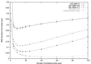
Figure 4: A plot showing slope estimation accuracy as a function of number of brightest pixels used for different detected photon arrival rates, given in the key in photons per sub-aperture per frame. The standard simulation parameters for this paper have been used, and the signal-to-noise ratio of each case (Eq. 2) is given in the legend.

3.3 Sensitivity to background subtraction

Images obtained from a WFS are typically calibrated before processing, which includes the removal of a background image. This background image must be obtained for each WFS exposure time and temperature to accurately remove the background. It is often the case that the background image used is not perfectly suited to the WFS images being obtained, and so systematic error results. For closed-loop AO systems, this error is small since the AO system is trying to minimise spot deviations. However for open-loop AO systems, wrong background subtraction leads to errors in wavefront slope estimation and so the wrong command vector is sent to the deformable mirror, reducing the AO correction. Here, this effect is investigated by incorrectly removing a background and investigating the slope estimation accuracy as the number of brightest pixels used is changed. We assume that $B_{\rm true}-B_{\rm subtracted}=N$ where $N$ is the same for each pixel, i.e. the background subtracted image still contains a constant background equal to $N$. Results are shown in Fig. 5 for values of $N$ equal to one, two and ten counts, i.e. the background map is wrong by this many photo-electrons. In these cases, the true slope measurement used for comparison (Eq. 1) does not contain the false background.

Figure 5: A plot showing slope estimation accuracy as a function of number of brightest pixels used for different background subtraction errors. The legend gives the error made in background subtraction, with 0 corresponding to no error, and 10 corresponding to a flat background of 10 counts remaining unsubtracted from the wavefront sensor images. The labels “(no subtraction)” and “(with subtraction)” refer to the brightest pixel algorithm used, either a simple threshold (removing all values below the $N^{th}$ brightest pixel), or a threshold and then subtracting the $N+1^{th}$ brightest pixel from unthresholded values respectively. Theoretically, the “with subtraction” curves are the same, the differences shown here being an artifact of the Monte-Carlo simulation.

It can be seen that the “$N+1^{th}$ subtracted algorithm” gives far better performance than the non-subtracted version because this effectively removes the false background. If this subtraction is not performed then estimation accuracy worsens as the unremoved background level is increased. Best results are obtained here by using 20 brightest pixels with the “$N+1^{th}$ subtracted algorithm”, far better than is achieved without using the brightest pixel selection.

3.4 Sensitivity to detector readout noise

In most AO systems, the detector readout noise of WFSs is generally fairly low since small signal levels often require detection, and are typically below 5 electrons. Since readout noise is random, it can have an impact on AO system performance if not taken into account. Fig. 6 shows slope estimation accuracy as a function of number of brightest pixels used for different detector readout noise levels. An important point to note here is that when readout noise is above about 5 electrons, subtracting the $N+1^{th}$ brightest pixel value leads to poorer performance than when no such subtraction is performed. This is because the higher readout noise means that the subtracted value varies significantly between frames since it contains this noise, and therefore a significantly different background is effectively subtracted for each frame. It should be noted that Fig. 6 shows results for when signal level is 200 photons per sub-aperture, while for higher signal levels the readout noise threshold at which subtraction of the $N+1^{th}$ brightest pixel should or should not be applied will be higher.

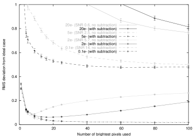
Figure 6: A figure showing slope estimation accuracy as a function of number of brightest pixels used for cases with different CCD readout noise. Comparisons for brightest pixel selection only, and using the “$N+1^{th}$ subtracted algorithm” are made. A light level of 200 detected photons per sub-aperture was assumed. The legend shows the signal-to-noise ratio (Eq. 2) for each readout noise.

For cases where the readout noise is a significant contribution, it may be possible to subtract an average of the $N+1$ to $N+M^{th}$ brightest pixels, with $M$ being a small positive integer, or by using a temporally filtered background level for each sub-aperture (i.e. averaging the $N+1^{th}$ brightest pixel over several frames), which would help to remove the random effect of readout noise. However, this is not investigated further here. These results show that selecting about 20 brightest pixels appears to give a reasonable performance for most readout noise levels, though a greater number of pixels could be advantageous when significant noise is present. For cases with sub-electron readout noise, such as that obtained when using an electron multiplying CCD (EMCCD) with high gain, estimation accuracy remains almost constant once more than about 20 pixels are selected, meaning that brightest pixel selection is not necessary (at least in this case, with 200 photons detected in each sub-aperture) though does no harm.

3.5 Changes in atmospheric conditions

The accuracy of wavefront slope measurement is sensitive to atmospheric conditions. Fig. 7(a) shows the how slope estimation accuracy changes for different atmospheric outer scale lengths ($L_{0}$). Selection of the 20 brightest pixels is about optimal in these cases, regardless of outer scale.

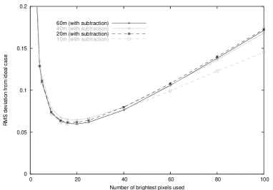
(a) (b)

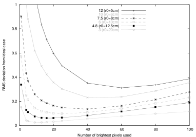
Figure 7: (a) A figure showing slope estimation accuracy as a function of number of brightest pixels used for different atmospheric outer scale lengths. (b) A figure showing slope estimation accuracy as a function of number of brightest pixels used for different atmospheric seeing conditions with $d/r_{0}$ given in the legend for $d=0.6$ m.

Similarly, Fig. 7(b) shows how estimation accuracy changes with atmospheric seeing (given by $d/r_{0}$ with $r_{0}$ being Fried’s parameter and $d=0.6$ m being the sub-aperture diameter. Here it can be seen that the optimal number of brightest pixels used depends strongly on the atmospheric seeing, but that for typical values seen during observing ($r_{0}=10-15$ cm), selecting 20 pixels gives good performance (along with subtraction of the 21st pixel value). In very bad seeing conditions, a greater number of pixels should be selected because the spots will be more diffuse.

3.6 Application to laser guide star elongated spots

So far, this paper has concentrated on application of brightest pixel selection based on un-elongated (natural guide star) Shack-Hartmann spots. However, the applicability with elongated laser guide star (1985A&A...152L..29F) spots should also be considered.

3.6.1 Rayleigh beacons

A Rayleigh laser guide star (as used with CANARY) is created by observing back scattered light from a laser beam as it transits through the atmosphere. By using a wavefront sensor with a fast shutter, it is possible to observe light scattered only from a small range of heights, thus creating a spot (artificial star) in the atmosphere. This spot will be geometrically elongated since it is not viewed along the direction of propagation, and the degree of elongation will be determined by the shutter time and the distance of the sub-aperture from the laser launch position (when mapped into the pupil plane). Using elongated Shack-Hartmann spots as would be seen by the CANARY LGS (Fig. 8(a)), the brightest pixel selection algorithm is investigated. The elongated spots shown give the expected elongation for a centre launched Rayleigh laser beacon at 20 km with shutter times that give a light transit distance of 0, 500, 1000 and 1500 m, viewed by a 60 cm sub-aperture at the edge of a 4.2 m telescope pupil. The spots have an unelongated width of 0.28 arcsec. A typical range gate depth for a Rayleigh beacon at this altitude is between 500–1000 m, and CANARY is likely to use a 600 m depth.

Fig. 8(b) shows the slope estimation accuracy as a function of number of brightest pixels selected, for different degrees of spot elongation. This figure shows accuracy in the direction parallel to the elongation, which has less sensitivity to wavefront slope than perpendicular to elongation and thus represents a worst case. The “$N+1^{th}$ subtracted algorithm” gives better performance than brightest pixel selection only and so only subtracted results are shown. This plot suggests that at least 20 brightest pixels should be selected, with more for very elongated spots. For a centre launched LGS, spot elongation is greater for sub-apertures at the edges of the WFSs. Therefore, the number of brightest pixels used may need to be adjusted according to sub-aperture location. Such an adjustment is possible with the DARC RTCS used with CANARY.

(a)
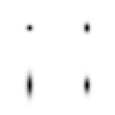
(b)

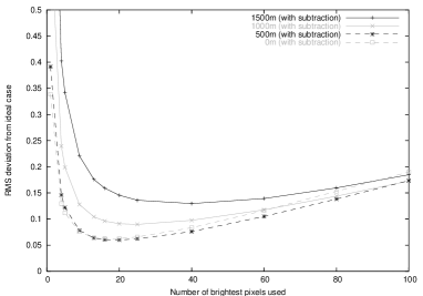
Figure 8: (a) A figure showing laser guide star elongations for different range gate depths, these being (clockwise from top left) 0 m, 500 m, 1000 m and 1500 m. The guide stars are assumed to be Rayleigh spots at an altitude of 20 km. (b) A figure showing slope estimation accuracy as a function of number of brightest pixels used for different laser guide star elongations. The key shows the range gate depth used for each case (i.e. the depth of the spot).

3.6.2 Sodium beacons

A Sodium LGS (1985A&A...152L..29F) is created using a laser tuned to a resonance of sodium atoms found in the mesosphere at about 90 km above the Earth’s surface. These atoms absorb laser light and then re-emit light in all directions when they decay, thus creating a signal that is detectable at the telescope. The density profile (with respect to altitude) of these atoms is known to vary with time (SodiumProfileData) meaning that the structure of the returned signal varies. As with a Rayleigh LGS, the spots will be geometrically elongated with the degree of elongation increasing with the distance between the laser launch telescope and the wavefront sensor sub-aperture in question. For the purposes of investigation here, we model the sodium layer as having a double Gaussian profile (SodiumDoublePeak), with one peak at 90 km and the other at a separation ($s$) above this, with $s$ ranging from 0–14 km. We assume peak sodium densities of 40% and 60% respectively with peak half-widths of 3.5 and 2 km. We consider the case of a sub-aperture placed 21 m from the laser launch telescope position with a 24 arcsec field of view, which gives elongations as shown in Fig. 9(a), with a $45^{\circ}$ rotation for display purposes, and assume a light level of 1000 detected photons per sub-aperture per frame. To investigate the performance of the brightest pixel selection algorithm, we show here results for which we are measuring wavefront slope in a direction parallel to spot elongation, which represents the worse case (least sensitive) scenario.

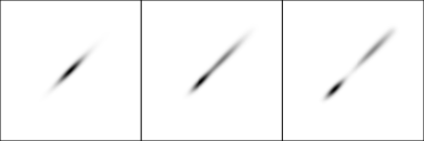
(a) (b)

Figure 9: (a) Sodium LGS sub-aperture images for different sodium profile peak separations (shown in negative). Separations of 0 km, 8 km and 14 km are shown, the double peak structure is clearly visible, and the surrounding box shows the sub-aperture size used here. (b) A figure showing slope esimation accuracy as a function of number of brightest pixels used for different sodium laser guide star models (double Gaussian model with varying peak separation). The legend gives the separation between the double peaks in the sodium profile. Subtraction of the $N+1^{th}$ brightest pixel has been applied, i.e. the “$N+1^{th}$ subtracted algorithm” has been used.

Fig. 9(b) shows the slope estimation accuracy as a function of number of brightest pixels selected using the “$N+1^{th}$ subtracted algorithm”, obtained using the method presented in § 2.2 for different double peaked sodium profiles. The presence of structure in the sodium spots means that these spots require greater numbers of brightest pixels to be selected than has previously been used to achieve best performance. Fig. 9(b) shows that selecting more than 100 brightest pixels in this case gives best performance, with more required when elongation increases. Elongation can be due to both the sodium layer profile and (as discussed previously) because of increasing distance of the sub-aperture from the laser launch position (increasing geometrical elongation). These results suggest that when using sodium laser guide stars, brightest pixel selection is beneficial (compared with the case for 256 pixels which corresponds to no selection), though care must be taken to select enough pixels.

3.7 Application to different sub-aperture sizes

Open-loop AO systems will generally have more pixels per sub-aperture than closed-loop systems, because spot motions are larger since the WFS does not see corrections made by the DM. So far, we have considered the case with $16\times 16$ pixels per sub-aperture, however it is interesting to see how brightest pixel selection performs with different numbers of pixels. Fig. 10 shows performance for different sub-aperture sizes as a function of number of brightest pixels used. This shows that for smaller sub-apertures, selecting fewer brightest pixels gives better performance, though if too few are selected, performance will be significantly degraded. For the smallest sub-apertures, there is little advantage in implementing the brightest pixel selection algorithm.

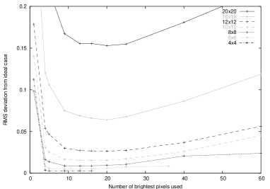
Figure 10: A figure showing slope estimation accuracy as a function of number of brightest pixels selected for different sub-aperture sizes (number of pixels per sub-aperture) as shown in the key. Subtraction of the next brightest pixel has been made.

It should be noted that although the curves representing sub-apertures with fewer pixels are lower, this does not mean that this will give better performance; rather it shows the performance that can be achieved relative to the noiseless case.

3.8 Linearity

Fig. 11(a) shows estimated wavefront slope across a noiseless sub-aperture using the brightest pixel selection algorithm for different numbers of selected pixels, as the slope across the sub-aperture is changed. Here, the “$N+1^{th}$ subtracted algorithm” has been implemented. It can be seen that there is significant non-linearity when small numbers of brightest pixels are selected, exemplified in the case using only the single brightest pixel. In this case, as the wavefront is gradually tilted causing the spot to move gradually across the sub-aperture, the brightest pixel will jump at fixed intervals from one pixel to the next, causing a jump in the corresponding slope estimation. When selecting more than one pixel, these jumps still occur, but as more and more pixels are selected the jumps become less profound. By the time 20 brightest pixels are selected, the change in estimated slope is almost linear.

(a) (b) (c)

Figure 11: (a) A figure showing wavefront slope measured using brightest pixel selection and subtraction of the next brightest pixel against the slope measured using all pixels (no selection). When few pixels are used, there are notable steps in slope estimation. Each trace has been offset vertically for clarity. From top to bottom, the number of brightest pixels are 1, 3, 4, 5, 7, 9, 10, 13, 20, 50, all (256). (b) A figure showing wavefront slope measured using brightest pixel selection and subtraction of the next brightest pixel after subtraction of slope measured using all pixels, against the slope measured using all pixels. Each trace has been offset vertically for clarity. From top to bottom the number of brightest pixels selected are 1, 9, 15, 20, 25, 50 and 100. (c) As for (b) but using brightest pixel selection only, without subtraction of the next brightest pixel.

Fig. 11(b) shows the estimated wavefront slope after subtraction of the slope calculated using all pixels, to show non-linearities more clearly. It should be noted that even with selection of 100 brightest pixels, the trace is not horizontal. This is due to the finite nature of the sub-aperture and the infinite size of the spot when all pixels are selected (an Airy disc pattern does not have a cut off beyond which all pixels are zero). Fortunately, because these traces are linear this is an effect that can be taken into account during the wavefront reconstruction (for example by scaling a control matrix by a small factor, or simply creating the control matrix using the same number of selected brightest pixels). Therefore, provided a large enough number of brightest pixels are selected (for example at least 20–25 in this case), the performance of the AO system will not be degraded.

Fig. 11(c) shows the linearity of the brightest pixel selection algorithm without subtraction of the $N+1^{th}$ brightest pixel, and this is considerably more non-linear than Fig. 11(b), suggesting that this subtraction should always be applied.

3.9 Computational complexity

The brightest pixel selection algorithm implemented in DARC for CANARY uses a quick-sort sorting algorithm, which on average makes $O\left(n\log n\right)$ comparisons (with a worst case $n^{2}$ comparisons), with $n$ being the number of pixels in a sub-aperture. This is repeated each iteration for each sub-aperture and so increases the AO system latency (the time between WFS readout and the DM shape being modified).

We have measured the latency when using and not using brightest pixel selection for the standard CANARY phase A configuration. We find that using brightest pixel selection adds about 330 $\mu$s to the latency of the system. These measurements were made using the software timing functions within DARC. Due to the configurable nature of DARC, we were able to optimise the number of processing threads used in each case, and optimum performance is obtained by increasing from 14 to 16 the number of threads when switching from no brightest pixel selection to brightest pixel selection.

When using brightest pixel selection, altering the number of pixels selected, and including subtraction of the next brightest does not affect the latency significantly, since most of the computation is in sorting the pixels which is performed regardless of the number of pixels used.

For CANARY, this latency increase does not significantly affect performance because latency is found to contribute only a small part of the overall error budget. However, for other systems, particularly higher order systems, this may have a significant affect, and so the benefits of brightest pixel selection should be weighted against the effect of increased latency.

3.10 Wavefront error reduction

The main purpose of an AO system is to remove residual wavefront error. For the default parameter set studied here, the results presented show an improvement of about 0.2 pixels RMS in slope estimation accuracy when comparing the pixel selection and traditional (no brightest pixel selection) algorithms. With a pixel scale of 0.22 arcsec per pixel this corresponds to 0.044 arcsec improvement, or, by considering phase across a 0.6 m diameter sub-aperture, about 130 nm of wavefront error.

We have performed full end-to-end Monte-Carlo simulations of CANARY using the Durham AO simulation platform (DASP) (basden5) and including the brightest pixel selection algorithm. These simulations included three off-axis natural guide star wavefront sensors with locations specified in table 12, and a DM in open-loop correcting an on-axis science path. With a 250 Hz update rate, we assume 200 detected photons per sub-aperture per frame (the default for this paper), and also assume a detector with two electron read noise, corresponding to an EMCCD with moderate multiplication gain. These parameters are chosen to match the default in the rest of this paper and to clearly show the advantage given by brightest pixel selection. The atmosphere model has a global $r_{0}$ of 12.5 cm and matches data taken on-sky with CANARY, namely, a strong ground layer (60% at 0m and 30% at 500 m), and a weaker layer (10% strength) at 5 km. Least-squares tomographic wavefront reconstruction was used by reconstructing phase at the layer heights, and then projecting phase down onto the on-axis open-loop DM.

Wavefront sensor	Radial offset	Angular offset
	/ arcsec	/ degrees
1	40.2	26.6
2	40.2	153.4
3	19.0	288.4
Science	0	0

Figure 12: Position of guide stars relative to on-axis location in a polar coordinate system.

Fig. 13 shows the estimated CANARY residual wavefront error as a function of number of brightest pixels selected (using the “$N+1^{th}$ subtracted algorithm”). It can be seen that brightest pixel selection can greatly reduce wavefront error, particularly in cases like this with a low or moderate signal-to-noise ratio. Without brightest pixel selection the simulation residual wavefront error is about 550 nm which gives a Strehl ratio of 6%, dominated by noise and tomographic error (a full CANARY error budget is given by (canaryresultsshort)). When 20 brightest pixels are selected the Strehl ratio increases to 33%, and the RMS WFS is reduced by about 270 nm to 280 nm. Therefore, for open-loop AO systems with large numbers of pixels per sub-aperture, brightest pixel selection can lead to significant performance improvement.

Figure 13: A figure showing residual wavefront error for an open-loop MOAO simulation based on CANARY, as a function of number of brightest pixels selected. Without brightest pixel selection, the error is about 550 nm.

4 Conclusion

The application of a threshold based on the $N^{th}$ brightest pixel in each sub-aperture of a Shack-Hartmann wavefront sensor has been investigated, with performance being studied for a wide range of parameters, with particular emphasis on linearity for application to open-loop AO, for example MOAO. This algorithm involves selecting the $N$ brightest pixels in each sub-aperture and setting to zero all pixels below this level. Additionally, it has been shown here that there is a significant gain in slope estimation accuracy and linearity if the $N+1^{th}$ pixel value is subtracted from all non-zero pixels.

From the results presented here, using the 20 brightest pixels (with subtraction of the 21${}^{\textrm{st}}$ brightest pixel seems optimal for average seeing, while more pixels, up to 40, should be used for poorer seeing, dependent on signal level and detector noise. One should always use more than about 10 brightest pixels otherwise performance will be significantly degraded. This technique is suited to Shack-Hartmann wavefront sensors with at least $4\times 4$ pixels per sub-aperture, and significant reductions in wavefront error can be achieved. Elongated laser guide star spots also require selection of a larger number of pixels.