Thickness–dependent magnetic structure of ultrathin Fe/Ir(001) films: from spin–spiral states towards ferromagnetic order

Abstract

We present a detailed study of the ground–state magnetic structure of ultrathin Fe films on the surface of fcc Ir(001). We use the spin-cluster expansion technique in combination with the relativistic disordered local moment scheme to obtain parameters of spin models and then determine the favored magnetic structure of the system by means of a mean field approach and atomistic spin dynamics simulations. For the case of a single monolayer of Fe we find that layer relaxations very strongly influence the ground-state spin configurations, whereas Dzyaloshinskii–Moriya (DM) interactions and biquadratic couplings also have remarkable effects. To characterize the latter effect we introduce and analyze spin collinearity maps of the system. While for two monolayers of Fe we find a single-$q$ spin spiral as ground state due to DM interactions, for the case of four monolayers the system shows a noncollinear spin structure with nonzero net magnetization. These findings are consistent with experimental measurements indicating ferromagnetic order in films of four monolayers and thicker.

I Introduction

By the end of the 20th century, in particular, since the birth of spintronics, thin films and nanostructures have gained increasing importance in industrial applications. The increasing demand for ultra-high density magnetic data storage devices had been one of the greatest driving forces of research and development involving nanostructures. With current hard disk technology approaching the superparamagnetic limit, the study of finite temperature magnetism in thin films and nanostructures is inevitable. Ab initio electronic structure methods give, in general, a very good description of the ground–state properties of solids. When trying to describe complex magnetic structures or finite temperature magnetism these methods are often used to generate parameters of spin models.

It is by now widely accepted that relativistic corrections to the Heisenberg model, especially the Dzyaloshinskii–Moriya (DM) interaction, play an important role in determining the magnetic ground state of some systems.bode-2007 ; ferriani-2008 ; udvardi-2008 ; antal-2008 Moreover, higher order interaction terms (multiple spin interactions) also have to be considered in many cases antal-2007 ; hardrat-2009 ; lounis-2010 to give an accurate description of magnetism. Very recent studies indicate that such interactions may even lead to the formation of exotic states like magnetic skyrmion lattices.heinze-2011

In the present work we demonstrate the use of spin models from first principles for the description of magnetism, in particular, determining the ground–state spin configuration of thin film systems. We use the spin-cluster expansion (SCE) combined with the relativistic disordered local moment (RDLM) theory to obtain model parameters. The SCE-RDLM method has just been successfully applied to the IrMn₃/Co(111) interface, a prototype for an exchange bias system, to calculate exchange interactions and magnetic anisotropies.szunyogh-2011

Here we go beyond the tensorial Heisenberg modeludvardi-2003 by including biquadratic couplings in the spin Hamiltonian and present our results for thin films of Fe on the (001) surface of fcc Ir. Previous theoretical studies have found that in case of a single Fe overlayer the favored magnetic configuration depends very strongly on layer relaxations, leading to the formation of spin spiral states near the experimental geometry.kudrnovsky-2009 We study the effect of layer relaxations on the magnetic interactions for the case of a monolayer, as well as the effect of higher order interactions on the spin configuration. We also examine thicker films consisting of two and four layers of Fe to see whether the bulk ferromagnetism of Fe emerges with increasing film thickness. Experiments have shown that thin films of Fe consisting of 4 or more monolayers produce a ferromagnetic signal in magneto-optic Kerr effect (MOKE) measurements with an in-plane easy axis.martin-2007 The results of our simulations turn to be consistent with the main experimental findings.

II Theory

II.1 Spin model

The most widely used ab initio methods to describe itinerant magnetic systems rely on the adiabatic approximation separating fast single–electron spin fluctuations from the slow transversal motion of the spins.antropov-1996 Furthermore, in the so-called rigid spin approximation it is assumed that longitudinal fluctuations of the local moments are negligible, so that the system of $N$ moments is characterized by a set of unit vectors $\left\{\vec{e}\right\}=\left\{\vec{e}_{1},\dotsc,\vec{e}_{N}\right\}$ describing the orientation of each local moment. Then the grand potential $\Omega\!\left(\left\{\vec{e}\right\}\right)$ of the system may be thought of as a classical spin Hamiltonian,gyorffy-1985 which can be used in numerical simulations to study the various magnetic properties of the system.

For practical applicability, the energy must be parametrized in a simple yet meaningful way. The most common approximation is a form of a generalized Heisenberg model,

$$\Omega\!\left(\left\{\vec{e}\right\}\right)=\Omega_{0}+\sum\limits_{i=1}^{N}\vec{e}_{i}\,\mathbf{K}_{i}\vec{e}_{i}-\frac{1}{2}\sum\limits_{\begin{subarray}{c}i,j=1\\ \left(i\neq j\right)\end{subarray}}^{N}\vec{e}_{i}\,\mathbf{J}_{ij}\vec{e}_{j},$$ (1)

where $\mathbf{K}_{i}$ and $\mathbf{J}_{ij}$ are the second order on-site anisotropy matrices and tensorial exchange couplings, respectively. The latter can be meaningfully decomposed into an isotropic component $J_{ij}^{I}=\operatorname{Tr}\mathbf{J}_{ij}/3$, an antisymmetric component $\mathbf{J}_{ij}^{A}$ and a traceless symmetric part $\mathbf{J}_{ij}^{S}$. The isotropic component describes a Heisenberg interaction, the antisymmetric part corresponds to the DM interactiondzyaloshinskii-1958 ; moriya-1960 in the form of

$$\vec{e}_{i}\;\mathbf{J}_{ij}^{A}\,\vec{e}_{j}=\vec{D}_{ij}\left(\vec{e}_{i}\times\vec{e}_{j}\right),$$ (2)

and the final component contributes to the so-called two-site anisotropy. In this paper we go beyond the second order expansion of Eq. (1) and include isotropic biquadratic interaction terms of the form $-B_{ij}\!\left(\vec{e}_{i}\cdot\vec{e}_{j}\right)^{2}$.

Even though a parametrization of the energy with a spin Hamiltonian possesses a much less direct connection to the magnetic properties of the system, it can be used well to simulate the magnetic behavior. One method for obtaining the parameters of the spin Hamiltonian directly from first principles calculations is the so-called spin-cluster expansion (SCE) combined with the relativistic disordered local moment scheme (RDLM).

II.2 Spin-cluster expansion

The spin-cluster expansion developed by Drautz and Fähnledrautz-2004 ; drautz-2005 gives a systematic parametrization of the adiabatic energy surface. Up to two-spin interactions, the grand potential may be expanded using real spherical harmonics as

$$\Omega\!\left(\left\{\vec{e}\right\}\right) \simeq\Omega_{0}+\sum\limits_{i}\sum\limits_{L\neq\left(0,0\right)}J_{i}^{L}Y_{L}\!\left(\vec{e}_{i}\right)$$

$$\quad+\frac{1}{2}\sum\limits_{i\neq j}\sum\limits_{L\neq\left(0,0\right)}\sum\limits_{L^{\prime}\neq\left(0,0\right)}J_{ij}^{LL^{\prime}}Y_{L}\!\left(\vec{e}_{i}\right)Y_{L^{\prime}}\!\left(\vec{e}_{j}\right),$$ (3)

where the summations do not include the constant spherical harmonic function of the composite index $\left(\ell,m\right)=\left(0,0\right)$. The coefficients in Eq. (3) are defined as

$$\Omega_{0} =\left\langle\Omega\right\rangle,$$ (4)

$$J_{i}^{L} =\int\mathrm{d}^{2}e_{i}\left\langle\Omega\right\rangle_{\!\vec{e}_{i}}Y_{L}\!\left(\vec{e}_{i}\right)$$ (5)

$$J_{ij}^{LL^{\prime}} =\int\mathrm{d}^{2}e_{i}\int\mathrm{d}^{2}e_{j}\left\langle\Omega\right\rangle_{\!\vec{e}_{i}\,\vec{e}_{j}}Y_{L}\!\left(\vec{e}_{i}\right)Y_{L^{\prime}}\!\left(\vec{e}_{j}\right),$$ (6)

where vectors in lower index indicate restricted averages, i.e., uniform directional averaging has to be carried out with respect to every spin in the system not noted in the lower index.

The terms of the spin Hamiltonian can be directly related to the terms of the SCE, for instance the isotropic biquadratic couplings can be expressed as

$$B_{ij} =-\frac{3}{8\pi}\sum\limits_{m=-2}^{2}J_{ij}^{(2,m)(2,m)}.$$ (7)

Clearly the key quantities of the SCE are the restricted directional averages of the grand potential.

II.3 Relativistic disordered local moment theory

The DLM scheme gives a description of a magnetic system in accordance with the adiabatic approximation. Its implementation within the Korringa-Kohn-Rostoker (KKR) theory was given by Györffy et al.,gyorffy-1985 with a relativistic generalization by Staunton et al.staunton-2004 ; staunton-2006 Combining it with the SCE provides a highly effective tool for determining the parameters of spin models. For a detailed presentation of the SCE-RDLM method see Ref. szunyogh-2011, . In the following we will review the most important features of the theory.

The electronic charge and magnetization densities are determined from a self-consistent-field KKR calculation. In good moment systems the magnitude of local moments may be considered as independent from their orientation. For a given set of self-consistent potentials, charge and local moment magnitudes, the orientations $\left\{\vec{e}\right\}$ of the local moments are accounted for by the similarity transformation of the single-site $t$-matrices,

$$\underline{t}_{i}\!\left(\vec{e}_{i}\right)=\underline{R}\!\left(\vec{e}_{i}\right)\underline{t}_{i}\!\left(\vec{e}_{z}\right)\underline{R}\!\left(\vec{e}_{i}\right)^{\dagger},$$ (8)

where $\underline{t}_{i}\!\left(\vec{e}_{z}\right)\equiv\underline{t}_{i}\!\left(\varepsilon;\vec{e}_{z}\right)$ is the $t$-matrix for a given energy, $\varepsilon$ (not labeled explicitly), with exchange field along the $z$ axis, and $\underline{R}\!\left(\vec{e}_{i}\right)$ is the representation of the $SO\!\left(3\right)$ rotation that transforms $\vec{e}_{z}$ into $\vec{e}_{i}$. Underlines denote matrices in the $\left(\kappa,\mu\right)$ angular momentum representation.

The coherent potential approximation (CPA) is employed to describe the magnetically disordered system. The strategy of the CPA is to substitute the disordered system with an effective (coherent) medium which is independent from the orientation of local moments, such that the scattering of an electron in the effective medium should resemble the average scattering in the disordered physical system. The scattering path operator of the effective medium is defined as

$$\underline{\underline{\tau}}_{c}=\left(\underline{\underline{t}}_{c}^{-1}-\underline{\underline{G}}_{0}\right)^{-1},$$ (9)

where double underlines denote matrices in site-angular momentum space, $\underline{\underline{G}}_{0}$ is the matrix of structure constants, and $\underline{\underline{t}}_{c}$ is site diagonal. Using the excess scattering matrices defined as

$$\underline{X}_{i}\!\left(\vec{e}_{i}\right)=\left[\left(\underline{t}_{c,i}^{-1}-\underline{t}_{i}^{-1}\!\left(\vec{e}_{i}\right)\right)^{-1}-\underline{\tau}_{c,ii}\right]^{-1}$$ (10)

the single-site CPA condition can be formulated as

$$\int\mathrm{d}^{2}e_{i}\,\underline{X}_{i}\!\left(\vec{e}_{i}\right)=\underline{0}.$$ (11)

Within validity of the magnetic force theorem the grand potential of the system can be expressed in terms of the excess scattering matrices and the related impurity matrices

$$\underline{D}_{i}\!\left(\vec{e}_{i}\right)= \left[\underline{I}+\left(\underline{t}_{i}^{-1}\!\left(\vec{e}_{i}\right)-\underline{t}_{c,i}^{-1}\right)\underline{\tau}_{c,ii}\right]^{-1}$$ (12)

for a given spin configuration and at zero temperature as

$$\Omega\!\left(\left\{\vec{e}\right\}\right) =\Omega_{c}-\frac{1}{\pi}\sum\limits_{i}\operatorname{Im}\int\limits^{\varepsilon_{F}}\mathrm{d}\varepsilon\,\ln\det\underline{D}_{i}\!\left(\vec{e}_{i}\right)$$

$$\quad-\frac{1}{\pi}\sum\limits_{k=1}^{\infty}\frac{1}{k}\sum\limits_{i_{1}\neq i_{2}\neq\dotsb\neq i_{k}\neq i_{1}}\operatorname{Im}\int\limits^{\varepsilon_{F}}\mathrm{d}\varepsilon\operatorname{Tr}\big{[}\underline{X}_{i_{1}}\!\left(\vec{e}_{i_{1}}\right)\underline{\tau}_{c,i_{1}i_{2}}$$

$$\qquad\times\underline{X}_{i_{2}}\!\left(\vec{e}_{i_{2}}\right)\dotsm\underline{X}_{i_{k}}\!\left(\vec{e}_{i_{k}}\right)\underline{\tau}_{c,i_{k}i_{1}}\big{]},$$ (13)

where the constant term reads as

$$\Omega_{c}=-\int\limits^{\varepsilon_{F}}\mathrm{d}\varepsilon\,N_{0}\!\left(\varepsilon\right)-\frac{1}{\pi}\operatorname{Im}\int\limits^{\varepsilon_{F}}\mathrm{d}\varepsilon\,\ln\det\underline{\underline{\tau}}_{c}\!\left(\varepsilon\right),$$ (14)

$N_{0}\!\left(\varepsilon\right)$ being the integrated density of states of free electrons. Eq. (13) can be used to calculate restricted averages of the grand potential for the SCE, Eqs. (4)–(6). In particular the two-site expansion terms are expressed as

$$J_{ij}^{LL^{\prime}} =-\frac{1}{\pi}\operatorname{Im}\int\limits^{\varepsilon_{F}}\mathrm{d}\varepsilon\iint\mathrm{d}^{2}e_{i}\;\mathrm{d}^{2}e_{j}\;Y_{L}\!\left(\vec{e}_{i}\right)Y_{L^{\prime}}\!\left(\vec{e}_{j}\right)$$

$$\qquad\times\operatorname{Tr}\ln\left[\underline{I}-\underline{X}_{i}\!\left(\vec{e}_{i}\right)\underline{\tau}_{c,ij}\underline{X}_{j}\!\left(\vec{e}_{j}\right)\underline{\tau}_{c,ji}\right],$$ (15)

implying that higher order two-site terms, such as biquadratic couplings, see Eq. (7), can be calculated just as easily as tensorial Heisenberg interactions.

III Results

III.1 Computational details

We used the screened Korringa–Kohn–Rostoker (SKKR) methodszunyogh-1994 ; zeller-1995 to perform self-consistent calculations for fcc bulk Ir and the layered Fe/Ir(001) systems. The in-plane lattice constant for the fcc lattice was chosen 2.715 Å.martin-2007 We used the local spin-density approximation parametrized according to Ceperley and Alder,ceperley-1980 and we employed the atomic sphere approximation with an angular momentum cutoff of $\ell_{\text{max}}=3$. A scalar-relativistic DLM description was used, corresponding to the paramagnetic state. Matrices of the effective CPA medium were determined to a relative error of 10^-5. We used 12 energy points on a semicircular path on the upper complex half-plane for the energy integrations, and 78 points were sampled in the irreducible wedge of the 2D Brillouin zone (BZ) for $k$-integrations.

The spherical integrations needed for the SCE, as in Eq. (15), were performed according to the Lebedev–Laikov scheme.lebedev-1999 The logarithm in Eq. (15) was expanded into a power series to avoid the phase problem due to the energy integration of the complex logarithm.

III.2 Fe₁/Ir(001)

Firstly we performed calculations for the case of an Fe monolayer. Along with the unphysical case of an unrelaxed Fe monolayer, systems with different layer relaxations were considered, namely 5%, 10%, 15% inward relaxations as well as the experimental value of -12% relaxation.martin-2007 According to Kudrnovský et al.,kudrnovsky-2009 we may expect a very strong dependence of exchange parameters on the layer relaxation, with a crossover of dominant Heisenberg couplings from ferromagnetic (FM) to antiferromagnetic (AFM). The obtained isotropic couplings are shown in Fig. 1.

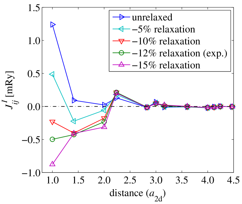
Figure 1: (Color online) Isotropic couplings for various layer relaxations in $\text{Fe}_{1}/\text{Ir}(001)$ as a function of interatomic distance in units of the in-plane lattice constant, $a_{\text{2d}}$.

While for the unrelaxed geometry all significant couplings are FM, with increasing inward relaxation the couplings for the three nearest neighbor (NN) shells become gradually AFM. For the case of experimental layer relaxation, the magnitude of the Heisenberg interactions is small and comparable up to four shells. While the tendency of the obtained curves is similar to those calculated by Kudrnovský et al.,kudrnovsky-2009 there are remarkable differences. In particular, at the experimental layer relaxation our largest isotropic couplings are 1 mRy smaller than those obtained in Ref. kudrnovsky-2009, , corresponding to a difference by a factor of three. Since the TB-LMTO-SGF method is known to give results that agree very well with KKR we use, we performed a series of check calculations to verify the reliability of our results. Increasing the numerical precision of the spherical integrations of the SCE, the convergence parameters of the CPA and the number of $k$ points for the BZ integration all resulted in identical isotropic couplings within linewidth. Increasing the number of energy points from 12 to 16 used for the energy integrations in the self-consistent calculations also leads to relative differences less then 2%.

We also performed calculations with spin-orbit coupling scaled to zeroebert-1996 as well as with the parametrization of the LDA according to Vosko, Wilk and Nusair.vosko-1980 The differences in the dominating exchange interactions from both sets of calculations were less then 0.1 mRy indicating that such factors are insufficient to explain the quantitative difference between our interactions and those of Kudrnovský et al.kudrnovsky-2009

Due to the frustrated nature and small magnitude of the isotropic exchange interactions it is possible that DM interactions or biquadratic couplings affect the ground–state spin configuration. The magnitude of these interactions for the first two NN shells is shown in Table 1. For higher relaxation values, in particular for the experimental one, the correction terms are indeed comparable to the isotropic couplings. Interestingly, in our case the biquadratic couplings all have positive sign indicating that these interactions favor collinear spin configurations. This feature implies a competition between the frustrated AFM exchange couplings, the DM and the biquadratic interactions, possibly leading to complex ground–state spin configurations.

Table 1: Calculated DM interactions and isotropic biquadratic couplings, see Eq. (7), in $\text{Fe}_{1}/\text{Ir}(001)$. All values are given in mRy units.

Layer relaxation		0%	-5%	-10%	-12%	-15%
$\left\lvert\vec{D}_{ij}\right\rvert$	1st shell	0.023	0.142	0.244	0.280	0.331
	2nd shell	0.156	0.207	0.209	0.198	0.170
$B_{ij}$	1st shell	0.110	0.109	0.088	0.077	0.059
	2nd shell	0.008	0.012	0.013	0.013	0.012

The Fourier transform of the tensorial coupling matrices was calculated to obtain the mean field estimate, as explained in the Appendix. In the monolayer case the Fourier transform is a $3\times 3$ tensor field defined on the two-dimensional BZ. The largest eigenvalue $J\!\left(\vec{q}\right)$ can be visualized as a surface in reciprocal space. The mean field estimate states that the maximum points of the surface give the characteristic spatial modulation of the ordered magnetic state, to which the paramagnetic state is unstable.

Reassuringly, the $J\!\left(\vec{q}\right)$ surface for the unrelaxed system has a pronounced maximum in the $\Gamma$ point of the BZ, indicating FM ground state. As the layer relaxation is increased, the corresponding surfaces are gradually depressed at the $\Gamma$ point, giving way to new maxima in general points of the Brillouin zone for -10% and larger inward relaxations. The contour plot of the $J\!\left(\vec{q}\right)$ surface for experimental layer relaxation is shown in Fig. 2. The maxima are around $\vec{q}=\left(0.5,0.7\right)\!\frac{\pi}{a_{\text{2d}}}$ and symmetry related points. This estimate suggests a complex noncollinear spin structure due to the frustrated and competing magnetic interactions detailed earlier. Note that there is an approximate degeneracy along lines connecting pairs of maxima. The difference between the maximum values of the surface and its value at, for instance, $\vec{q}=\left(0.6,0.6\right)\!\frac{\pi}{a_{\text{2d}}}$ is less then 0.03 mRy. This implies the possibility that the actual ground state of the system is somewhere along these degenerate lines, but not necessarily in the precise maxima of the surface.

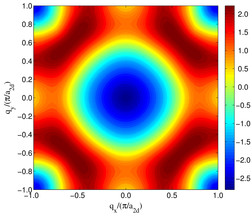
Figure 2: (Color online) $J\!\left(\vec{q}\right)$ surface for Fe₁/Ir(001) with experimental relaxation. The color coding in units of mRy is shown on the right.

The effect of relativistic tensorial interactions may be assessed by calculating the $J\!\left(\vec{q}\right)$ surface using only the isotropic part of the exchange tensors. In doing so, the shape of the resulting surface is the same, however its maxima are shifted closer to the zone boundary, to $\vec{q}=\left(0.45,0.85\right)\!\frac{\pi}{a_{\text{2d}}}$ and related points. The degeneracy of the line connecting the maxima is remarkably decreased. Based on the mean field estimate, the ground–state spin configuration of Fe₁/Ir(001) is a spin spiral, the periodicity of which is largely affected by the DM interactions.

We performed zero temperature Landau–Lifshitz–Gilbert spin dynamics simulations to verify the mean field prediction and to reveal the influence of biquadratic couplings on this noncollinear spin structure. Due to the expected noncollinear structures we used a $128\times 128$ lattice of spins along with free boundary conditions to prevent the appearance of spurious periodicity. Interactions were included up to 7 two-dimensional lattice constants ($a_{\text{2d}}$). For every relaxation two kinds of simulations were performed, one with and the other without biquadratic coupling terms. Every simulation was initialized from a random spin configuration, the same for simulations with and without biquadratic terms. All simulations were continued until there was no measurable difference (i.e., less than $10^{-6}$ mRy) in the total interaction energy of the system. It should be noted that on-site anisotropy was not included in the simulations due to its small size (0.06 mRy in case of experimental layer relaxation), however two-site anisotropy was included as the symmetric part of the $\underline{\underline{J}}_{ij}$ tensors.

In the case of unrelaxed geometry, the simulations led to (out-of-plane) FM order as expected. As layer relaxation is introduced, the transition predicted by the mean field estimates is reflected in the spin dynamics simulations as well, as the ground states become complex spin-spirals for relaxations of - 10% and above. The Fourier components of the emergent spin configurations agree very well with the mean field estimates. Interestingly, for -15% relaxation the spin configuration of the simulated system contains a huge number of domains with various orientations for the spin spirals, which is in very good agreement with the degeneracy of the $J\!\left(\vec{q}\right)$ surface along the corresponding $\vec{q}$ points.

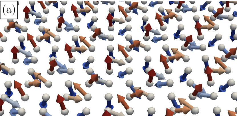
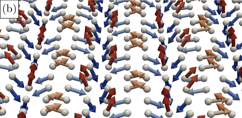
Figure 3: (Color online) Ground–state spin configurations of the Fe monolayer with experimental layer relaxation (a) without and (b) with biquadratic couplings.

It is expected that biquadratic couplings can significantly affect the ground–state spin configuration when the tensorial Heisenberg interactions alone lead to the formation of noncollinear spin structures. This is the case for the experimental layer relaxation for which the resulting spin-configurations of the two simulations are shown in Fig. 3. The lattice Fourier transform of the spin configuration in Fig. 3a has a peak at $\vec{q}\approx\left(0.719,0.495\right)\!\frac{\pi}{a_{\text{2d}}}$, which perfectly coincides with the numerical maximum of the corresponding $J\!\left(\vec{q}\right)$ surface. Interestingly the peak for the simulation including biquadratic terms is at $\vec{q}\approx\left(0.735,0.500\right)\!\frac{\pi}{a_{\text{2d}}}$, which is only very slightly different from the previous value. Even though the two spin structures in Fig. 3 seem very different, their spatial modulation is almost identical. The main reason for this is that while in Fig. 3b there is a clear two row-by-two row periodicity along one direction, in Fig. 3a we can see a helical spiral along the same direction with $90^{\circ}$ angle between adjacent spins. Both orderings have a period of $4a_{\text{2d}}$.

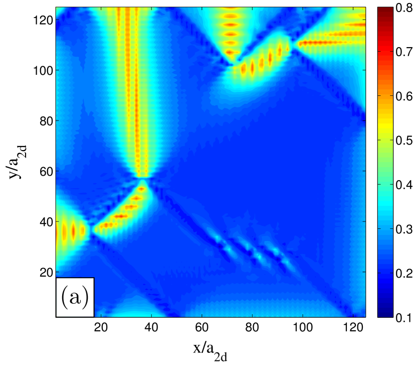
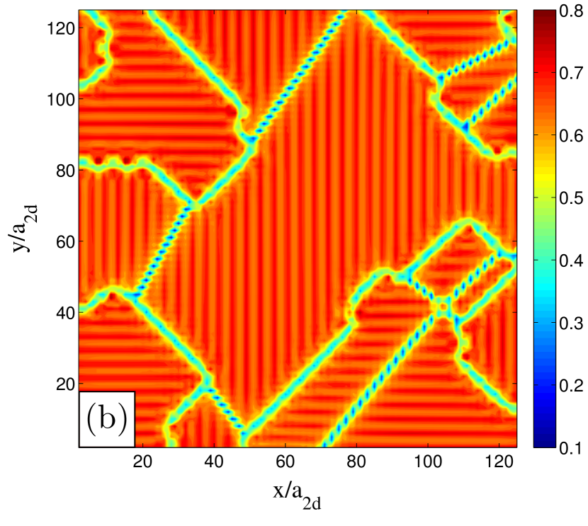
Figure 4: (Color online) Collinearity map for the approximate ground state of Fe₁/Ir(001) with experimental layer relaxation, (a) without and (b) with biquadratic couplings. The color coding in units of mRy is shown on the right.

We may try to grasp the effect of biquadratic interactions based on the real space spin structure. From the form of the biquadratic coupling between two specific spins, $-B_{ij}\left(\vec{e}_{i}\cdot\vec{e}_{j}\right)^{2}$, it is clear that a coupling with positive sign favors collinear alignment, either parallel or antiparallel. It is motivated that positive biquadratic couplings acting on a noncollinear spin configuration will try to increase the collinearity within the system.

Let us define the collinearity of two spins as

$$\operatorname{coll}\!\left(\vec{e}_{i},\vec{e}_{j}\right)=\frac{2}{\pi}\left\lvert\arccos\left(\vec{e}_{i}\cdot\!\vec{e}_{j}\right)-\frac{\pi}{2}\right\rvert,$$ (16)

which is simply the deviation of the angle between the two spins from a right angle, normalized between 0 and 1, 1 indicating most collinear arrangement (i.e., where $\vec{e}_{i}\cdot\vec{e}_{j}=\pm 1$). Using this definition we may create a collinearity map of any spin configuration, plotting at each site an averaged collinearity defined as

$$\operatorname{coll}\!\left(i\right)=\frac{1}{z_{i}}\sum\limits_{\begin{subarray}{c}j\\ \left\langle i,j\right\rangle\end{subarray}}\operatorname{coll}\!\left(\vec{e}_{i},\vec{e}_{j}\right),$$ (17)

where the summation includes every first NN of site $i$ and correspondingly $z_{i}$ stands for the coordination number of site $i$. The reason for the consideration of only first NN sites is, besides practicality, the rapid spatial decay of biquadratic couplings, suggesting that this interaction is mainly sensitive to the first NN collinearity.

Using the above definitions, the calculated collinearity maps from the two kinds of simulations are shown for experimental relaxation in Fig. 4. The difference between the two maps is remarkable. At first glance we can see that the two configurations have a completely different domain structure. While in Fig. 4a there are smoothly connected domains of low collinearity (0.22 on average), in Fig. 4b we can see neatly separated, homogeneous domains of high collinearity (0.67 on average). This is a clear indication that biquadratic couplings have a serious effect on the magnetic structure in this specific system.

III.3 Fe₂/Ir(001)

Martin et al.martin-2007 found using MOKE measurements that Fe films of 4 monolayers or thicker produce an in-plane FM signal at room temperature. For the case of an Fe monolayer with reasonable layer relaxations the theoretically predicted spin spiral states have zero net magnetization, thus they would not provide a MOKE signal. To see if the bulk-like behavior of Fe emerges for thicker films, we extended our studies to cases of two and four monolayers of Fe on Ir(001).

The geometries of Fe_n/Ir(001), both for $n=2$ and $n=4$ were assumed according to Ref. martin-2007, , with the minor simplification that no layer relaxation was applied to the Ir substrate. As shown in Fig. 5, the isotropic Heisenberg couplings we obtained show a strong FM coupling between the two layers, while the intralayer couplings are smaller, and in case of the subsurface layer the dominant ones are AFM. It should be mentioned that the DM interactions are one order of magnitude smaller then the isotropic terms, and the biquadratic couplings are even smaller by one order.

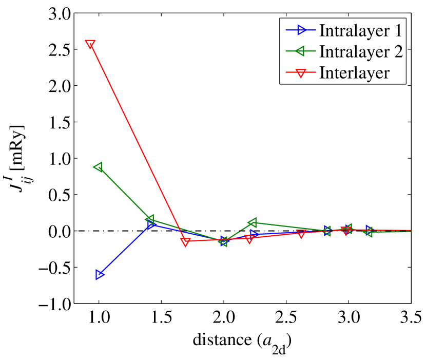
Figure 5: (Color online) Isotropic Heisenberg couplings in $\text{Fe}_{2}/\text{Ir}(001)$ as a function of interatomic distance in units of the in-plane lattice constant, $a_{\text{2d}}$.

The $J\!\left(\vec{q}\right)$ surface for the bilayer has its maximum near the $\Gamma$ point, but not exactly at the zone center. There is a degenerate circle at $\left\lvert\vec{q}\right\rvert\approx 0.07\frac{\pi}{a_{\text{2d}}}$ where the surface is maximal, predicting a long wavelength spin spiral. Considering only the isotropic part of the exchange tensors the corresponding surface has its maximum in the $\Gamma$ point. This indicates that the DM interaction imposes a noncollinear spin structure on the otherwise FM system.

Since the number of neighbors within the same radius rapidly increases with the number of Fe layers, the spin dynamics simulations for the multilayers were performed with in-plane system sizes of $64\times 64$ sites. Fig. 6 shows the resulting spin configuration of the surface Fe layer for the simulation including biquadratic couplings. Note that due to the strong FM interlayer coupling the subsurface layer displays a very similar pattern.

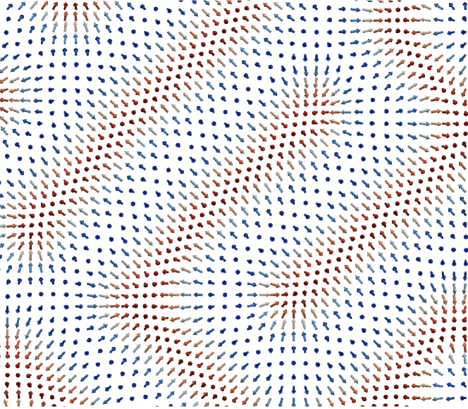
Figure 6: (Color online) Approximate ground–state spin configuration of Fe₂/Ir(001), surface layer shown from the top. Arrows are colored according to $z$ component, ranging from red (up) to blue (down).

The Fourier transform of the spin configuration indicates that the propagation direction of the spin spirals is not exactly diagonal, since the wave vector is $\vec{q}=\left(0.13,0.16\right)\!\frac{\pi}{a_{\text{2d}}}$ (and symmetry related points). The fact that $\vec{q}$ is not along any high symmetry lines is consistent with the degeneracy seen on the $J\!\left(\vec{q}\right)$ surface, however, the magnitude of the wave vector is twice as large as that of the mean field estimate. This quantitative difference can mainly be attributed to the flaws of the mean field approach, but we can not rule out finite size effects in the spin dynamics simulation.

The simulation without biquadratic interactions resulted in a very similar pattern indicating that these interactions are irrelevant in thicker films due to increased isotropic Heisenberg couplings. Simulations performed using only the isotropic part of the Heisenberg tensors led to the appearance of large FM domains without the spin spiral pattern seen in Fig. 6. This result is corroborated by several previous observations that the DM interaction may significantly affect the ground–state spin configuration, and even lead to the formation of spin spirals in thin film systems.ferriani-2008 ; udvardi-2008 It is also interesting to note that a very similar labyrinth pattern was found in a monolayer of Mn on W(001).ferriani-2008 Composed of single-$q$ cycloidal spin spirals, the configuration shown in Fig. 6 does not have a net magnetic moment.

III.4 Fe₄/Ir(001)

In the following, for the case of four monolayers of Fe, the Fe layers are going to be indexed from the substrate to the surface, so that layer 1 is closest to the Ir substrate and layer 4 is the surface layer. Summarizing the calculated interactions, the interlayer isotropic Heisenberg couplings are strong and FM, with increasing magnitude towards layers closer to the surface. Interestingly the couplings between intralayer first nearest neighbors are mostly weakly antiferromagnetic, only the two layers closest to the substrate show couplings of considerable magnitude, above 1 mRy in absolute value. The corrections to the Heisenberg spin-model are weak. Only the first NN intralayer DM vectors in layer 1 are larger than 0.1 mRy, and the strongest biquadratic couplings are around 0.07 mRy. Based on these features it is probable that the magnetic behavior is dominated by isotropic couplings.

The $J\!\left(\vec{q}\right)$ surface for Fe₄/Ir(001) shown in Fig. 7 has its maximum in the $\Gamma$ point, anticipating FM arrangement. If the ground state is indeed FM, it is worth looking at the mean field estimate for the Curie temperature. The maximum of the surface with 10.89 mRy corresponds to a mean field estimate of $T_{C}=573$ K. As mean field approximations overestimate the stability of the ordered phases due to neglected fluctuations, the actual critical temperature is surely lower than this value. Still, it is possible that at room temperature the system is in the ordered phase.

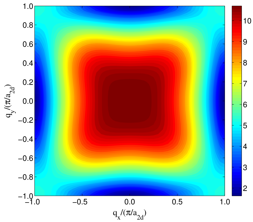
Figure 7: (Color online) $J\!\left(\vec{q}\right)$ surface for Fe₄/Ir(001). The color coding in units of mRy is shown on the right.

The spin dynamics simulations revealed that the ground state is more complicated than what the mean field approach predicts. The simulated system converged into a complex spin structure regardless of the presence of biquadratic coupling terms. In each layer the spins formed a cycloidal spiral of $\vec{q}=\left(0.41,0.41\right)\!\frac{\pi}{a_{\text{2d}}}$ rotating in a vertical plane, but with an additional in-plane FM modulation leading to nonzero net magnetization, $\left\langle\vec{e}_{i}\right\rangle\neq 0$. While the wave vector of the spiral is the same within every layer due to the strong interlayer coupling, the magnitude of the FM Fourier component increases with distance from the substrate. For a quantitative comparison of the net magnetizations, the layer-averaged magnetizations calculated from a homogeneous domain containing 1178 spins are presented in Table 2. The average magnetization, $\left\langle\vec{e}_{i}\right\rangle$, is clearly in-plane and monotonically increasing in magnitude towards the surface where it reaches a value larger than 0.7. Considering the actual size of each magnetic moment, also shown in Table 2, the total average magnetic moment of the system is 1.27$\mu_{\text{B}}$.

Table 2: Layer-resolved averaged magnetizations, $\left\langle\vec{e}_{i}\right\rangle$, and atomic magnetic moments in a given domain of Fe₄/Ir(001) containing 1178 spins.

	$\left\langle\vec{e}_{i}\right\rangle$	magnetic moment [$\mu_{\text{B}}$]
layer 1	$\left(0.26,0.26,0.01\right)$	1.98
layer 2	$\left(0.37,0.37,0.01\right)$	2.02
layer 3	$\left(0.51,0.53,0.00\right)$	1.60
layer 4	$\left(0.54,0.57,0.00\right)$	2.71

In contrast to bulk bcc Fe, the net magnetization points along the $\left(110\right)$ direction, i.e., towards intralayer second-nearest neighbors, but it is indeed in-plane. Possibly in even thicker films we would see FM order with easy axis along the (100) direction, as was found experimentally.

IV Conclusions

We used the recently developed SCE-RDLM method to obtain spin Hamiltonians from ab initio calculations, going beyond the anisotropic Heisenberg model by including isotropic biquadratic interaction terms. The obtained interaction parameters allow for a detailed investigation of the magnetic ground state via a mean field approach and atomistic spin dynamics simulations. We presented results for Fe thin films on the (001) surface of a semi-infinite Ir substrate. For the case of an Fe monolayer we found that layer relaxations drastically rearrange the interaction landscape, leading to the appearance of complex non-collinear spin structures. Relativistic corrections, in particular, Dzyaloshinskii-Moriya interactions, are needed to be taken into account as anisotropic couplings largely affect the ground state. Spin dynamics simulations also revealed that including biquadratic interactions to the spin model significantly alters the ground state spin configuration by favoring a more collinear state. This serves as an instructive warning that in some systems the usual Heisenberg model might give an insufficient description of magnetic properties.

For thicker films of two and four monolayers we found that biquadratic couplings are irrelevant in determining the ground–state spin configuration due to the large magnitude of the Heisenberg interaction. While the bilayer system still produces a single-$q$ spin spiral as ground state due to the DM interaction, in the quadrilayer system there is nonzero net magnetization superimposed on a cycloidal spin structure. This finding may be consistent with experimental results showing a ferromagnetic signal in MOKE measurements above four monolayers of Fe deposited on Ir(001).

*

Appendix A Mean field paramagnetic spin susceptibility

For a system of spins $\left\{\vec{e}\right\}$ governed by the grand potential $\Omega\left(\left\{\vec{e}\right\}\right)$, the best variational mean field trial Hamiltonian $\Omega_{0}\left(\left\{\vec{e}\right\}\right)=-\sum_{i}\vec{h}_{i}\vec{e}_{i}$, i.e., the one that minimizes the free energy is given by

$$\vec{h}_{i}=-\frac{3}{4\pi}\int\mathrm{d}^{2}e_{i}\;\vec{e}_{i}\left\langle\Omega_{0}\right\rangle^{0}_{\vec{e}_{i}},$$ (18)

where the angle brackets now denote thermodynamic averaging with respect to the mean field probability distribution $P_{0}\!\left(\left\{\vec{e}_{i}\right\}\right)=\exp\left[-\beta\Omega_{0}\!\left(\left\{\vec{e}_{i}\right\}\right)\right]/Z_{0}$, $Z_{0}$ being the corresponding canonical partition function.

For our spin model extended with an inhomogeneous external field,

$$\Omega\!\left(\left\{\vec{e}\right\}\right) =\Omega_{0}+\sum\limits_{i=1}^{N}\vec{e}_{i}\,\mathbf{K}_{i}\vec{e}_{i}-\frac{1}{2}\sum\limits_{\begin{subarray}{c}i,j=1\\ \left(i\neq j\right)\end{subarray}}^{N}\vec{e}_{i}\,\mathbf{J}_{ij}\vec{e}_{j}$$

$$\quad-\frac{1}{2}\sum\limits_{\begin{subarray}{c}i,j=1\\ \left(i\neq j\right)\end{subarray}}B_{ij}\!\left(\vec{e}_{i}\cdot\vec{e}_{j}\right)^{2}-\sum_{i=1}^{N}\vec{h}_{i}^{\text{ext}}\cdot\vec{e}_{i},$$ (19)

the Weiss field reads as

$$\vec{h}_{i}=\vec{h}_{i}^{\text{MF}}+\vec{h}_{i}^{\text{ext}},$$ (20)

where the molecular field induced by the interaction takes on the familiar mean field form,

$$\vec{h}_{i}^{\text{MF}}=\sum\limits_{j\left(\neq i\right)}\mathbf{J}_{ij}\vec{m}_{j},$$ (21)

$\vec{m}_{j}=\left\langle\vec{e}_{j}\right\rangle^{0}$ being the average magnetization at site $j$. Note that neither the on-site anisotropy nor the biquadratic couplings contribute to the Weiss field.

The spin susceptibility, defined as $\chi_{ij}^{\alpha\beta}=\partial m_{i}^{\alpha}/\partial h_{j}^{\text{ext,$\beta$}}$ may be related to the susceptibility of the non-interacting spin system $\chi_{ij}^{0,\alpha\beta}=\partial m_{i}^{\alpha}/\partial h_{j}^{\beta}$ as

$$\bm{\chi}_{ij}=\bm{\chi}_{ij}^{0}+\sum\limits_{k\neq l}\bm{\chi}_{ik}^{0}\mathbf{J}_{kl}\bm{\chi}_{lj}.$$ (22)

For layered systems with only two-dimensional translation invariance we may separate site indices according to a layer index and an in-plane index,

$$\bm{\chi}_{IJ,ij}=\bm{\chi}_{IJ,ij}^{0}+\sum\limits_{\begin{subarray}{c}K,L,k,l\\ (K,k)\neq(L,l)\end{subarray}}\bm{\chi}_{IK,ik}^{0}\,\mathbf{J}_{KL,kl}\bm{\chi}_{LJ,lj},$$ (23)

where capital indices denote layers. Due to in-plane translation invariance we may introduce the two-dimensional Fourier transform of the quantities, for instance

$$\bm{\chi}_{IJ}\!\left(\vec{q}\right)=\sum\limits_{\vec{R}_{i}}\bm{\chi}_{IJ,i0}\operatorname{e}^{-\imath\vec{q}\vec{R}_{i}},$$ (24)

which might be thought of as blocks of matrices in layer and Cartesian space,

$$\left[\widehat{\bm{\chi}}\!\left(\vec{q}\right)\right]_{IJ}=\bm{\chi}_{IJ}\!\left(\vec{q}\right).$$ (25)

Using this notation we may easily invert Eq. (23) and arrive at

$$\widehat{\bm{\chi}}\!\left(\vec{q}\right) =\left(\widehat{\mathbf{I}}-\widehat{\bm{\chi}}^{0}\!\left(\vec{q}\right)\widehat{\mathbf{J}}\!\left(\vec{q}\right)\right)^{-1}\widehat{\bm{\chi}}^{0}\!\left(\vec{q}\right),$$ (26)

indicating an enhancement of the spin susceptibility due to the Heisenberg interaction. In the paramagnetic limit this simplifies to

$$\widehat{\bm{\chi}}\!\left(\vec{q}\right) =\left(3k_{B}T\widehat{\mathbf{I}}-\widehat{\mathbf{J}}\!\left(\vec{q}\right)\right)^{-1}.$$ (27)

Annealing the system from the paramagnetic phase there will be a temperature, $T_{\text{ord}}$, where $\widehat{\bm{\chi}}\!\left(\vec{q}\right)$ becomes singular, indicating that the paramagnetic phase is unstable to the formation of some magnetically ordered state at that temperature. This transition temperature $T_{\text{ord}}$ is given by the condition

$$T_{\text{ord}} =\frac{1}{3k_{B}}\max\limits_{\vec{q}}\left\{\text{eigenvalues of $\widehat{\mathbf{J}}\!\left(\vec{q}\right)$}\right\}$$

$$=\frac{1}{3k_{B}}\max\limits_{\vec{q}}J\!\left(\vec{q}\right),$$ (28)

and the corresponding $\vec{q}$ where this happens gives the characteristic wave vector of the ordered phase (where the $\vec{q}$ vectors are sought for in the two-dimensional BZ). In Eq. (28) we introduced the notation $J\!\left(\vec{q}\right)$ for the maximal eigenvalue of $\widehat{\mathbf{J}}\!\left(\vec{q}\right)$ at a given wave vector. We may gain valuable insight regarding magnetic ordering in the system by plotting this scalar function against the points of the BZ.

References

- (1) M. Bode, M. Heide, K. von Bergmann, P. Ferriani, S. Heinze, G. Bihlmayer, A. Kubetzka, O. Pietzsch, S. Blügel, and R. Wiesendanger, Nature 447, 190 (2007).
- (2) P. Ferriani, K. von Bergmann, E. Y. Vedmedenko, S. Heinze, M. Bode, M. Heide, G. Bihlmayer, S. Blügel, and R. Wiesendanger, Phys. Rev. Lett. 101, 027201 (2008).
- (3) L. Udvardi, A. Antal, L. Szunyogh, Á. Buruzs, and P. Weinberger, Physica B 403, 402 (2008).
- (4) A. Antal, B. Lazarovits, L. Balogh, L. Udvardi, and L. Szunyogh, Phil. Mag. B 88, 2715 (2008).
- (5) A. Antal, L. Udvardi, B. Újfalussy, B. Lazarovits, L. Szunyogh, and P. Weinberger, J. Magn. Magn. Mater. 316, 118 (2007).
- (6) B. Hardrat, A. Al-Zubi, P. Ferriani, S. Blügel, G. Bihlmayer, and S. Heinze, Phys. Rev. B 79, 094411 (2009).
- (7) S. Lounis and P. H. Dederichs, Phys. Rev. B 82, 180404(R) (2010).
- (8) S. Heinze, K. von Bergmann, M. Menzel, J. Brede, A. Kubetzka, R. Wiesendanger, G. Bihlmayer, and S. Blügel, Nature Physics 7, 713 (2011).
- (9) L. Szunyogh, L. Udvardi, J. Jackson, U. Nowak, and R. Chantrell, Phys. Rev. B 83, 024401 (2011).
- (10) L. Udvardi, L. Szunyogh, K. Palotas, and P. Weinberger, Phys. Rev. B 68, 104436 (2003).
- (11) J. Kudrnovský, F. Máca, I. Turek, and J. Redinger, Phys. Rev. B 80, 064405 (2009).
- (12) V. Martin, W. Meyer, C. Giovanardi, L. Hammer, K. Heinz, Z. Tian, D. Sander, and J. Kirschner, Phys. Rev. B 76, 205418 (2007).
- (13) V. P. Antropov, M. I. Katsnelson, B. N. Harmon, M. van Schilfgaarde, and D. Kusnezov, Phys. Rev. B 54, 1019 (1996).
- (14) B. L. Györffy, A. J. Pindor, J. B. Staunton, G. M. Stocks, and H. Winter, J. Phys. F: Met. Phys. 15, 1337 (1985).
- (15) I. Dzyaloshinskii, J. Phys. Chem. Solids 4, 241 (1958).
- (16) T. Moriya, Phys. Rev. 120, 91 (1960).
- (17) R. Drautz and M. Fähnle, Phys. Rev. B 69, 104404 (2004).
- (18) R. Drautz and M. Fähnle, Phys. Rev. B 72, 212405 (2005).
- (19) J. B. Staunton, S. Ostanin, S. S. A. Razee, B. L. Györffy, L. Szunyogh, B. Ginatempo, and E. Bruno, Phys. Rev. Lett. 93, 257204 (2004).
- (20) J. B. Staunton, L. Szunyogh, Á. Buruzs, B. L. Györffy, S. Ostanin, and L. Udvardi, Phys. Rev. B 74, 144411 (2006).
- (21) L. Szunyogh, B. Újfalussy, P. Weinberger, and J. Kollár, Phys. Rev. B 49, 2721 (1994).
- (22) R. Zeller, P. H. Dederichs, B. Újfalussy, L. Szunyogh, and P. Weinberger, Phys. Rev. B 52, 8807 (1995).
- (23) D. M. Ceperley, and B. J. Alder, Phys. Rev. Lett. 45, 566 (1980).
- (24) V.I. Lebedev, and D.N. Laikov, Doklady Mathematics 59, 477 (1999).
- (25) H. Ebert, H. Freyer, A. Vernes, and G.-Y. Guo, Phys. Rev. B 53, 7721 (1996).
- (26) S. H. Vosko, L. Wilk, and M. Nusair, Can. J. Phys. 58, 1200 (1980).