Mixed RG Flows and Hydrodynamics at Finite
Holographic Screen

Abstract

We consider quark-gluon plasma with chemical potential and study renormalization group flows of transport coefficients in the framework of gauge/gravity duality. We first study them using the flow equations and compare the results with hydrodynamic results by calculating the Green functions on the arbitrary slice. Two results match exactly. Transport coefficients at arbitrary scale is ontained by calculating hydrodynamics Green functions. When either momentum or charge vanishes, transport coefficients decouple from each other.

I Introduction

In the application of AdS/CFT Maldacena:1997re , calculations are usually done on the holographic screen at infinity. However, according to the renormalization group (RG) ideas kraus ; Susskind ; verlinde , those are the UV fixed point values which can not be reached by experiments performed at the finite energy scale. Therefore we need to run them down to the scale where one actually performs the experiment by the renormalization group flow. Recent studies of Wilsonian approach Joe.RG ; Hong.RG to holographic RG flow of transport coefficients Sin:2011yh in the framework of gauge/gravity duality suggest that those apparently different approaches of sliding membrane Hong.Membrane , Wilsonian fluid/gravity Andy.RG and holographic Wilsonian renormalization group (HWRG)Joe.RG ; Hong.RG ; Wilson:RG are equivalent Sin:2011yh . Some of the transport coefficients such as shear viscosity $\eta$, AC conductivity and diffusion constant $D$ have non-trivial radial flows so that they interpolate the horizon values son2 and the boundary values son1 smoothly. The holographic Wilsonian RG is also useful to understand the low energy effective theory for holographic liquid Faulkner:2009wj ; Joe.Semiholography ; Son.Deconstruction .

Since the discussions so far has been mostly for zero charge cases, one natural question is how to extend it to the case with finite chemical potentials. Unlike the zero charge case, metric fluctuation and Maxwell fluctuation will mix in charged black hole background. In general, the mixing effect of metric and Maxwell fluctuations in charged black hole is of essential importance, since it is the reason why transverse vector modes of Maxwell fields can diffuse and longitudinal Maxwell modes can have sound modes in the presence of the charge. Part of the answer has been given in Andy.RG where the cutoff dependence of diffusion constant for the shear part of metric perturbations was calculated. The authors achieved it without explicit decoupling procedure by taking a specific scaling which, somehow, effectively decouples the mixed modes. However, it is not clear how to understand why it happens and what scaling limit should be taken for other (i.g. sound) modes.

In this paper, we first establish the flow equations of transport coefficients in the presence of chemical potential and numerically integrate the flow equations. We then calculate transport coefficients directly by hydrodynamic calculation on the holographic screen at finite radial position and compare the two results. We will find complete agreement.

This paper is organized as follows. In section II, we will briefly review the holographic RG flow of transport coefficients. We also derive the running diffusion constant in zero charged black hole from sliding membrane which reproduces the previous result in Andy.RG obtained by scaling method. In section III, we set up the charged black hole medium and focus on mixing structure of metric and Maxwell perturbations. We emphasize on organizing the coupled equations of motion. In section IV, we first write down the decoupled flow equation for both electric conductivity and “conductivity” for momentum current at zero momentum. And then we worked out the “conductivity” for momentum current in diffusion scaling limit following Andy.RG . We write down the complete mixed flow equations for electric conductivity, momentum current “conductivity” and mixing parameter in the end of this section. In section V, we use the hydrodynamical method to calculate the Green functions at finite screen $r=r_{c}$. We obtained the transport coefficients from Green functions by Kubo formula and we found complete agreement with the results from flow equations in section IV. We conclude in last section.

II Holographic Renormalization Group and Running transport coefficients: A review

In this section, we shall discuss a few approaches to RG flow of transport coefficients and discuss the equivalence between them: They are sliding membrane paradigm Hong.Membrane , Wilsonian fluid/gravity Andy.RG and Holographic Wilsonian RG Joe.RG ; Hong.RG . The radial flow for transport coefficients can be derived from holographic Wilsonian RG equation. It can also be derived from the classical equation of motion. The idea of membrane paradigm is to consider a membrane action Parikh:1997ma coming from the boundary action at sketched horizon. Similarly sliding membrane Hong.Membrane paradigm uses the boundary action at arbitrary slice. From that action, one can obtain the retarded Green function by solving the equation of motion perturbatively in hydrodynamic regime. The linear response theory then gives the transport coefficients. The Green functions and transport coefficients satisfy the same radial evolution coming from holographic Wilsonian effective action $S_{B}$, which in turn can be obtained from integrating out UV geometry directly Hong.RG ; Sin:2011yh . $S_{B}$ can also be treated as a boundary action at cutoff slice and it induces multi-trace deformations for IR dynamics Joe.RG ; Hong.RG . For more discussions about the essential multi-trace deformations see Witten:2001ua ; Vecchi:2010dd . If one define the linear level transport coefficient at cut off slice, then the Hamilton-Jacobi equation for the effective action can directly give radial flow of them. These flows are exactly the same as those coming from equations of motion as explicitly shown in Sin:2011yh .

Technically, sliding membrane paradigm is more convenient than holographic Wilsonian RG simply because the former starts from equation of motion while the latter is conceptually more satisfactory. We shall mostly use the former in this paper.

We briefly review the sliding membrane paradigm Hong.Membrane below. We derive the cutoff dependent diffusion constant, which is also calculated from the Wilsonian approach of Fluid/Gravity Andy.RG . We show that the result from the sliding membrane paradigm reproduces that in Andy.RG to demonstrate the equivalence of sliding membrane paradigm Hong.Membrane and Wilsonian approach of Fluid/Gravity Andy.RG . We start with standard Maxwell action

$$S=-\int d^{d+1}x\sqrt{-g}{1\over 4g_{\text{eff}}^{2}(r)}F_{MN}F^{MN}\ ,$$ (1)

with the background metric

$$ds^{2}=-g_{tt}dt^{2}+g_{rr}dr^{2}+g_{ii}dx^{i}dx^{i}\ .$$ (2)

Defining $J^{\mu}$ and $G$ by

$$J^{\mu}=-{1\over g_{\text{eff}}^{2}}\sqrt{-g}F^{r\mu}\ ,\quad G=\sqrt{-g}/g_{\text{eff}}^{2}\ ,$$ (3)

equations of motion can be written as 

$$\partial_{t}J^{t}+\partial_{z}J^{z} = 0\ ,$$ (4)

$$\partial_{r}J^{t}+Gg^{tt}g^{zz}\partial_{z}F_{zt} = 0\ ,$$ (5)

$$\partial_{r}J^{z}-Gg^{tt}g^{zz}\partial_{t}F_{zt} = 0\ ,$$ (6)

where $z$ is the momentum direction and we focus on the longitudinal mode first. The Bianchi identities are given by:

$$-{g_{rr}g_{zz}\over G}\partial_{t}J^{z}-{g_{rr}g_{tt}\over G}\partial_{z}J^{t}+\partial_{r}F_{zt}=0\ .$$ (7)

Using the definition of the conductivity $\sigma=J^{z}/E_{z}=J^{z}/F_{zt}$, we have

$$\partial_{r}\sigma={\partial_{r}J^{z}F_{zt}-J^{z}\partial_{r}(F_{zt})\over F_{zt}^{2}}\ ,\quad\sigma^{2}={(J^{z})^{2}\over(F_{zt})^{2}}\ .$$ (8)

We want to replace all the $\partial_{r}$ terms in above equation using equations of motion. Taking use of (4), (6) and (7), all the currents and fields disappear and finally we have the flow for conductivity Hong.Membrane

$${\partial_{r}\sigma\over i\omega}=g^{2}_{\text{eff}}\sigma^{2}\left[{1\over\sqrt{-g}g^{rr}g^{zz}}-{k^{2}\over\omega^{2}}{1\over\sqrt{-g}g^{rr}g^{tt}}\right]-{1\over g^{2}_{\text{eff}}}\sqrt{-g}g^{tt}g^{zz}\ .$$ (9)

Before doing explicit analysis for this conductivity flow we should mention that there are two important scaling limits for the frequency dependent flow equations: one is $\omega\sim k^{2}<<1$ and the other is $k=0,\omega<<1$. In the diffusion scaling regime $\omega\sim k^{2}<<1$, we have following solution of (9) for conductivity :

$${1\over\sigma(r_{c})}={1\over\sigma_{H}}-{k^{2}\over i\omega}{1\over f_{0}}\ ,\quad\quad{1\over f_{0}}=\int_{r_{H}}^{r_{c}}{g^{2}_{\text{eff}}\over\sqrt{-g}g^{rr}g^{tt}}\ .$$ (10)

Since the (complex) conductivity at arbitrary slice and the green function is related by

$$\sigma^{ij}(k_{\mu},r_{c})=-{G_{R}^{ij}({k_{\mu},r_{c}})\over i\omega}\ ,$$ (11)

we can write the Green function at cutoff surface in terms of horizon conductivity $\sigma_{H}$

$$G_{R}^{ii}({k_{\mu},r_{c}})={\omega^{2}\sigma_{H}\over i\omega-D(r_{c})k^{2}}\ ,$$ (12)

where $D(r_{c})=\sigma_{H}/f_{0}\$ is the cutoff dependent diffusion constant. Substituting into (10), we have

$${1\over\sigma(r_{c})}={1\over\sigma_{H}}-{k^{2}\over i\omega}{D(r_{c})\over\sigma_{H}}\ .$$ (15)

In the orthonormal frame, we have the normalized momentum as follows

$$\omega\rightarrow\omega_{c}\equiv{\omega\over\sqrt{g_{tt}}}\ ,\quad k\rightarrow k_{c}\equiv{k\over\sqrt{g_{ii}}}\ .$$ (16)

Using these new variables we can rewrite (10) as

$${1\over\sigma(r_{c})}={1\over\sigma_{H}}-{k_{c}^{2}\over i\omega_{c}}{\hat{D}(r_{c})\over\sigma_{H}}\ ,$$ (17)

where $\hat{D}(r_{c})$ is given by

$$\hat{D}(r_{c})\equiv D(r_{c}){g_{ii}\over\sqrt{g_{tt}}}\ .$$ (18)

Defining the local temperature by $T_{c}={T_{H}\over\sqrt{g_{tt}}}\ ,$ and a dimensionless diffusion constant by $\bar{D}_{c}\equiv\hat{D}T_{c}$, we have

$${\bar{D}_{c}\over T_{c}}={\sigma_{H}g_{ii}\over f_{0}\sqrt{g_{tt}}}\ .$$ (19)

This is precisely the result obtained in Andy.RG , supporting the equivalence of two approaches. So far we considered only chargeless case. It is known that presence of charge introduces non-trivial mixing between modes. We will consider what happens for the flow of charged black hole below.

III Mode mixing in Charged AdS Black hole

In order to describe low energy physics of various strongly coupled systems, we need different IR deformations for the $d+1$ dimensional AdS background. Consider a $d$ dimensional holographic system with finite charge density. The minimal $d+1$ bulk action is

$$S=\int d^{d+1}x\sqrt{-g}\left[{1\over 2\kappa^{2}}\left({R}+{d(d-1)\over L^{2}}\right)-{1\over 4g^{2}}F^{2}\right]\ ,$$ (20)

where Newton constant $G_{N}=\kappa^{2}/8\pi$ and $g$ is the Maxwell coupling. Maxwell and Einstein equations are given by

$$\partial_{\mu}(\sqrt{-g}F^{\mu\nu}) = 0,\;\;$$ (21)

$${1\over\kappa^{2}}\left(R_{\mu\nu}-{1\over 2}g_{\mu\nu}{R}-g_{\mu\nu}{d\ (d-1)\over 2L^{2}}\right) = {1\over 2g^{2}}\left(2F_{\mu\rho}F_{\nu}^{\rho}-{g_{\mu\nu}\over 2}F_{\rho\sigma}F^{\rho\sigma}\right)\ .$$ (22)

The charged black hole solution for this action is

$$ds^{2} = {r^{2}\over L^{2}}\left(-f(r)dt^{2}+dx^{i}dx^{i}\right)+{L^{2}\over r^{2}}{dr^{2}\over f(r)}\ ,$$ (23)

$$\bar{A}_{t} = \mu\left(1-{r_{0}^{d-2}\over r^{d-2}}\right)\ ,\quad f(r)=1+\alpha Q^{2}{r_{0}^{2d-2}\over r^{2d-2}}-(1+\alpha Q^{2}){r_{0}^{d}\over r^{d}}\ .$$ (24)

where $\alpha={L^{2}\kappa^{2}\over(d-1)(d-2)g^{2}}$ is a dimensionless coupling. Chemical potential $\mu$ is related to $Q$ by $Q={\mu(d-2)\over r_{0}}$ and the horizon $r_{0}$ is the largest root of $f(r)=0$.

III.1 Modes in RN-AdS

We consider the perturbations

$$g_{\mu\nu}\rightarrow g_{\mu\nu}+\delta g_{\mu\nu},\quad A_{\mu}\rightarrow A_{\mu}+\delta A_{\mu}\ ,$$ (25)

around the background $g_{\mu\nu}$ and $A_{\mu}$, which are given in $(\ref{metric})$ and $(\ref{metric1})$. One can use background metric raise and lower tensor indices. The linearized gravity fluctuations can be decomposed into tensor, vector and scalar type Kodama:2000fa ; Kovtun:2005ev . We will consider the first two types and leave the last one elsewhere. In the charged black hole background, vector part of metric perturbation and transverse Maxwell perturbation will couple. We can organize the the former such that its action and equations look like that of longitudinal Maxwell perturbation. For more details about the action of linearized fluctuations in RN-AdS, see Ge:2008ak ; Edalati:2010hk .

III.1.1 Tensor Mode $\delta g^{x}_{y}$

By symmetry argument or by direct analysis one can find that off-diagonal perturbation $\phi\equiv\delta g^{x}_{y}$ decouples from all other perturbations. Thus it satisfies the same equation of motion to that for a minimally coupled massless scalar:

$$\partial_{\mu}(\sqrt{-g}\partial^{\mu}\phi)=0\ .$$ (26)

This evolution for $\phi$ will give the flow of correlation of the corresponding operator $T_{x}^{y}$. Notice that if we work in $d=3$, we should take $k\rightarrow 0$ limit since we only have two spatial directions.

III.1.2 Vector Modes $\delta g^{x}_{z},\delta g^{x}_{t},\delta g^{x}_{r},\delta A_{x}$

Picking up a momentum parallel to $z$ direction, we can only have $d-2$ transverse dimension left. One can observe that the shear mode of metric perturbations of components $g_{xz},g_{xt},g_{xr}$ which behave similarly as Maxwell field $a_{z},a_{t},a_{r}$ son2 ; Hong.Membrane defined by

$$a_{z}\equiv\delta g^{x}_{z},\quad a_{t}\equiv\delta g^{x}_{t},\quad a_{r}\equiv\delta g^{x}_{r}\ .$$ (27)

In terms of these variables, finally the vector part off shell action in $d+1$ dimensional RN-AdS can be written as follows:

$$S=\int d^{d+1}x\;\sqrt{-g}\left(-\frac{1}{4g^{2}}F^{\mu\nu}F_{\mu\nu}-\frac{1}{4g^{2}_{\text{eff}}(r)}f^{\mu\nu}f_{\mu\nu}+\frac{1}{g^{2}}a_{t}A^{\prime}_{x}{\bar{A}}^{\prime}_{t}\right)\ .$$ (28)

Here we have used $j$ and $f$ to denote the current and strength for the $a_{\mu}$:

$$j^{\mu}=-{1\over g_{\text{eff}}^{2}(r)}\sqrt{-g}f^{r\mu}\ ,\quad f_{\mu\nu}=\partial_{\mu}a_{\nu}-\partial_{\nu}a_{\mu}\ ,$$ (29)

and $J$ and $F$ to denote the current and strength for $A_{\mu}$. Consider first the chargeless case, equations of motion for shear part metric fluctuations can be written as

$$\partial_{t}j^{t}+\partial_{z}j^{z} = 0$$ (30)

$$\partial_{r}j^{t}+Gg^{tt}g^{zz}\partial_{z}f_{zt} = 0$$ (31)

$$\partial_{r}j^{z}-Gg^{tt}g^{zz}\partial_{t}f_{zt} = 0\ ,$$ (32)

where the effective determinant and the effective coupling are

$$G=\sqrt{-g}/g^{2}_{\text{eff}}(r)\ ,\quad{1\over g^{2}_{\text{eff}}(r)}={g_{xx}\over 2\kappa^{2}}\ .$$ (33)

For the charged-AdS black hole, we introduce the new charge density which is defined as

$$\tilde{j^{t}}=j^{t}-\frac{1}{g^{2}}\sqrt{-g}{\bar{A}}^{\prime}_{t}A_{x}\ .$$ (34)

The equations of motion takes the same form as chargeless case,

$$\partial_{t}\tilde{j^{t}}+\partial_{z}j^{z} = 0$$ (35)

$$\partial_{r}\tilde{j^{t}}+Gg^{tt}g^{zz}\partial_{z}f_{zt} = 0$$ (36)

$$\partial_{r}j^{z}-Gg^{tt}g^{zz}\partial_{t}f_{zt} = 0\ ,$$ (37)

but $j^{t}$ is replaced by $\tilde{j}^{t}$, while the Bianchi identity holds as before

$$-{g_{rr}g_{zz}\over G}\partial_{t}j^{z}-{g_{rr}g_{tt}\over G}\partial_{z}j^{t}+\partial_{r}f_{zt}=0\ .$$ (38)

Defining $J^{x}$ and $\tilde{J}^{x}$ by

$$J^{x}=-\frac{1}{g^{2}}\sqrt{-g}g^{rr}g^{xx}\partial_{r}A_{x}\ ,\quad\tilde{J}^{x}=J^{x}+\frac{1}{g^{2}}\sqrt{-g}{\bar{A}}^{\prime}_{t}a_{t}$$ (39)

the equation of motion for $A_{x}$ can be written as

$$-\partial_{r}\tilde{J^{x}}+\frac{1}{g^{2}}\sqrt{-g}g^{xx}(-g^{tt}\partial_{t}F_{tx}+g^{zz}\partial_{z}F_{zx})=0\ .$$ (40)

III.1.3 Vector Mode $A_{x}$ at $k_{z}=0$

From (40) and (36), one can see that $A_{x}$ decouples from $a_{t}$ in the $k_{z}\to 0$ limit:

$$\partial_{r}(\sqrt{-g}g^{rr}g^{xx}\partial_{r}A_{x})-\frac{1}{g^{2}}\sqrt{-g}g^{2}_{\text{eff}}({\bar{A}}^{\prime}_{t})^{2}A_{x}+\omega^{2}\sqrt{-g}g^{xx}g^{tt}A_{x}=0\ .$$ (41)

The relevant on-shell action for $A_{x}$ at boundary $r=r_{c}$ can be written as

$$S_{\text{on-shell}}=\int_{r=r_{c}}\tilde{J}^{x}A_{x}\ .$$ (42)

IV Flows of Transport Coefficients

We shall establish the transport coefficient flows for the charged black hole in this section.

IV.1 Shear Viscosity Flow and Scalar Response

Since tensor mode decouples from all other perturbations, it behaves as a massless scalar perturbation even in the charged black hole background. Following the sliding membrane argument Hong.Membrane , it is useful to define a cutoff dependent scalar response function

$$G_{\phi}(r_{c},k_{\mu})={-\sqrt{-g}g^{rr}\partial_{r}\phi\over 2\kappa^{2}\phi(r_{c},k_{\mu})}\ .$$ (43)

And we define

$$\eta(r_{c},k_{\mu}):={G_{\phi}(r_{c},k_{\mu})\over i\omega}$$ (44)

which satisfies a flow equation evolving equation of motion at $k=0$:

$${\partial_{r_{c}}\eta(r_{c},\omega)}=i\omega\left({2\kappa^{2}\eta^{2}(r_{c},\omega)\over\sqrt{-g}g^{rr}}-\frac{\sqrt{-g}g^{tt}}{2\kappa^{2}}\right)\ .$$ (45)

It is manifest from above equation that in the zero frequency limit, $\eta(r_{c})$ is independent of $r_{c}$. Its value is request to be

$$\eta(r_{c})=\eta(r_{0})={1\over 16\pi G}\left(\frac{r_{0}}{L}\right)^{d-1},$$ (46)

by the horizon regularity. Since the entropy density is $s=\frac{1}{4G}\left(\frac{r_{0}}{L}\right)^{d-1}$, the ratio $\eta/s$ does not run. In the next section we will see that this is consistent with the direct calculation of $\eta(r_{c})$ using the holographic hydrodynamics at the finite holographic screen.

IV.2 Electric conductivity flow at the zero momentum

Now we shall consider the conductivity flow coming from $A_{x}$ perturbation with zero momentum. From (42) one can obtain the conjugate momentum for $A_{x}(r)$ at $r=r_{c}$

$$\Pi_{A_{x}}(r_{c})={\delta S_{\text{on-shell}}\over\delta\ A_{x}}=J^{x}+\frac{1}{g^{2}}\sqrt{-g}{\bar{A}}_{t}^{\prime}a_{t}\ .$$ (47)

Notice that this is nothing but the shifted current ${\tilde{J}}^{x}$ which was introduced previously to simplify the equation of motion. As explained in Hartnoll:2009sz , the first and second term in right hand side of (47) should be related to electric conductivity and thermal-electric conductivity respectively. Notice that the on-shell action is the integral over the membrane at $r=r_{c}$ and the conjugate momentum eq.(47) is also defined at $r_{c}>r_{0}$. In the limit of zero momentum, $A_{x}$ decouples and we can define electric conductivity by

$$\sigma_{A}(\omega,r_{c}):={J^{x}\over i\omega A_{x}}\ .$$ (48)

One can quickly rewrite the equation of motion (41) as flow equation for $\sigma_{A}$:

$${\partial_{r_{c}}\sigma_{A}\over-i\omega}+{g^{2}\sigma_{A}^{2}\over\sqrt{-g}g^{rr}g^{xx}}+{g^{2}_{\text{eff}}\sqrt{-g}(\bar{A}^{\prime}_{t})^{2}\over{g^{2}}\omega^{2}}-\frac{1}{g^{2}}\sqrt{-g}g^{xx}g^{tt}=0\ .$$ (49)

Due to the regularity condition at the horizon, we need

$$\sigma_{H}\equiv\sigma_{A}(r_{0})={1\over g^{2}}\left({r_{0}\over L}\right)^{d-3}\ ,$$ (50)

which is consistent with horizon conductivity evaluated in Hong.Membrane . In order to see the solutions explicitly, we plot the conductivity flows with different black hole charges in $d=3$ in Figure 1.

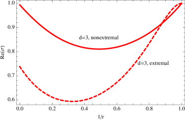
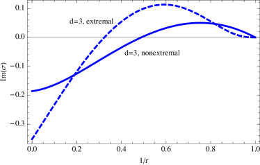
Figure 1: $r$ flow of AC conductivity, with $d=3$ RN-AdS black hole background. Here we normalize $r$ such that the horizon localizes at $r=1$.

A few remarks are in order for these flow solutions.

• Zero Charge Limit: Remember that the charge density in the boundary theory is related to the chemical potential by

  $$\rho=\mu r_{0}^{d-2}/g^{2}\ .$$ (51)

  When $\mu=0$ chargeless case, the $d=3$ conductivity is independent of the cutoff position. The flow solution for $d=3$ is trivial while there are nontrivial flow solutions for $d\neq 3$ Sin:2011yh . When $d\neq 3$ there is a fixed point at boundary but not at horizon. This is because near the boundary metric is aysmptotically AdS and scale invariance is there. This scale invariance is lost when two fluctuating modes mix in the RN-AdS black hole case.

• Extremal Limit: As shown in Figure 1, when the charged AdS black hole becomes extremal, one can find a fixed point from flow of conductivity near the horizon due to the appearance of AdS₂ near the horizon. This fixed point will disappear in non-extremal case. One should notice that there is no fixed point for the conductivity near the boundary both for extremal and non-extremal case. The evolution equation for $\sigma_{A}$ loses scale invariance near the infinite boundary in the presence of charge due to the mix of $a_{t},A_{x}$ modes.

• Check against Boundary Result: In order to check the consistence with previous results calculated at infinite boundary $r=\infty$, we plot the boundary AC conductivity in Figure 2, which is precisely consistent with the results in Hartnoll:2009sz . The $Q$ dependent term in the flow equation clearly give the origin for the divergence of the imaginary part of the conductivity in the zero frequency limit.

• Conductivity Minimum: It is interesting to observe that there is a window of parameters $\omega$ and $\mu$ where the real part of conductivity curve in radial direction has a minimum as shown in Figure 1. The minimum of the conductivity pick up a certain scale $r_{*}$ and we show the charge dependence of that scale in Figure 2.

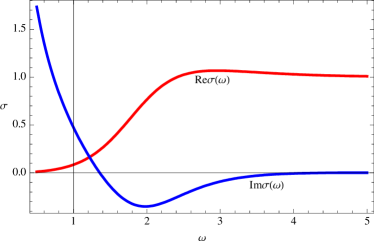
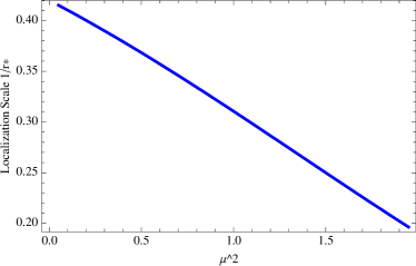
Figure 2: Left: Frequency dependence of boundary AC conductivity, with $d=3$ RN-AdS black hole background . As a check for our flow solutions, the boundary AC conductivity is precisely consistent with the results in  Hartnoll:2009sz . Right: Chemical potential dependence of scale $r_{*}$ with minimal conductivity in $d=3$ RN-AdS, where $\mu$ is dimensionless chemical potential.

IV.3 RG flow of ‘Conductivity’ of momentum current flow at zero momentum

Since the metric perturbation $a_{\mu}$ mimic the Maxwell system, we can define the “conductivity” for the mode $a_{z}=h^{x}_{z}$ by

$$\sigma_{h}:={j^{z}\over f_{zt}}\ .$$ (52)

At $k_{z}=0$, since $a_{\mu}$ modes are decoupled with $A_{x}$, we can obtain the decoupled flow of $\sigma_{h}$ as follow

$${\partial_{r}\sigma_{h}\over-i\omega}+\sigma_{h}^{2}\ {g_{rr}g_{zz}\over G}-Gg^{tt}g^{zz}=0\ .$$ (53)

This flow equation has the same form as the longitudinal conductivity flow in zero charge case although the metric components contain $Q$ dependence. As a consistent check, this flow equation is exactly the same as shear viscosity flow in (45), because when $k_{z}=0$, there is no polarization direction and $\sigma_{h}$ is nothing but shear viscosity by definition. We will explain more about the physical mean of $\sigma_{h}$ in next subsection.

IV.4 RG flow of ‘Conductivity’ of momentum current in diffusion region

Since shear parts of metric perturbations behaves as longitudinal Maxwell field with a $r$ dependent effective coupling, we shall work out the “conductivity” flow in diffusion region. In order to handle the equations of motion: (35)$\sim$(38), we write them in momentum space and take the diffusion scaling following Andy.RG

$$\partial_{t} \sim \epsilon^{2}\ ,\quad\partial_{z}\sim\epsilon$$ (54)

$$f_{zt} \sim \epsilon^{3}\left({f_{zt}}^{(0)}+\epsilon{f_{zt}}^{(1)}+\dots\right)\ .$$ (55)

First consider the in-falling boundary condition, which requires $j^{z}$ linearly related to $f_{zt}$ near the horizon. This condition requires us to scale $j^{z}$ as same power of $f_{zt}$:

$$j^{z}\sim\epsilon^{3}\left({j^{z}}^{(0)}+\epsilon{j^{z}}^{(1)}+\dots\right)\ .$$ (56)

Through the charge conservation equation we obtain

$$\tilde{j^{t}}\sim\epsilon^{2}\left(\tilde{j^{t}}^{(0)}+\epsilon\tilde{j^{t}}^{(1)}+\dots\right)\ ,$$ (57)

and we can also obtain

$${j^{t}}\sim\epsilon^{2}\left({j^{t}}^{(0)}+\epsilon{j^{t}}^{(1)}+\dots\right)\ ,$$ (58)

since there is no different scaling between $j^{t}$ and $\tilde{j^{t}}$. Now we want to take $\epsilon\rightarrow 0$ limit, and only the lowest orders of fields are left. From (36) and (37) we obtain

$$\partial_{r}\tilde{j^{t}}^{(0)}=0\ ,\quad\partial_{r}{j^{z}}^{(0)}=0\ .$$ (59)

Requiring charge conservation, we have

$${j^{z}}^{(0)}=\tilde{j^{t}}^{(0)}{k\over\omega}\ .$$ (60)

From (38), we have

$$\partial_{r}f^{(0)}_{zt}={g_{rr}g_{tt}\over G}\partial_{z}{j^{t}}^{(0)}\ .$$ (61)

It means we have the solution for $f^{(0)}_{zt}$

$$f^{(0)}_{zt}(r)=f^{(0)}_{zt}(r_{0})+2\kappa^{2}\int_{r_{0}}^{r}dr{g^{2}\partial_{z}{j^{t}}^{(0)}(r)\over\sqrt{-g}g^{rr}g^{tt}g_{xx}}\ .$$ (62)

Following the usual definitions in sliding membrane for chargeless case, we define the conductivity by current and electric field as

$$\sigma_{h}(r_{c}):={{j^{z}}^{(0)}(r_{c})\over f^{(0)}_{zt}(r_{c})}={k\over\omega}{\tilde{j^{t}}^{(0)}(r_{c})\over f^{(0)}_{zt}(r_{c})}\ .$$ (63)

Remember

$$\tilde{j^{t}}^{(0)}={j^{t}}^{(0)}-\frac{1}{g^{2}}\sqrt{-g}A^{(0)}_{x}\bar{A}^{\prime}_{t}$$ (64)

is a constant. By taking the scaling limit we have the simplified equation of motion for $A^{(0)}_{x}$:

$$\partial_{r}(\frac{1}{g^{2}}\sqrt{-g}g^{rr}g^{xx}\partial_{r}A^{(0)}_{x})=g^{2}_{\text{eff}}\bar{A}^{\prime}_{t}{j^{t}}^{(0)}(r)\ .$$ (65)

The solution for $A^{(0)}_{x}$ can be solved explicitly as shown in Andy.RG .

Since ${j^{z}}^{(0)}$ is a constant in radial direction, after having the solution for $A^{(0)}_{x}$, (62) can be rewritten as

$${1\over\sigma_{h}(r_{c})}={1\over\sigma_{h}(r_{0})}-{k_{c}^{2}\over i\omega_{c}}{\bar{D}_{h}(r_{c})/T_{c}\over\sigma_{h}(r_{0})}\ ,$$ (66)

where the horizon value is

$$\sigma_{h}(r_{0})={1\over 16\pi G_{N}}\left({r_{0}\over L}\right)^{d-1}\ .$$ (67)

This is exactly the “conductivity” flow for shear part of metric fluctuations. This is our main result in this subsection. After taking the scaling limit following Andy.RG , we have the analytical result for RG flow of “conductivity” of momentum current.

As a byproduct, we obtain the $\bar{D}_{h}$ as

$$\bar{D}_{h}(r_{c})={1\over 4\pi}{(d-2)(1-\alpha Q^{2})+2\over(1+\alpha Q^{2})d-2(d-1)\alpha Q^{2}(r_{0}/r_{c})^{d-2}}\ ,$$ (68)

which is charge dependent diffusion constant. Notice that we have used the solution for $A_{x}$ to obtain the $\bar{D}_{h}$. This result was first obtained in Andy.RG , where the diffusion constant is derived from Fick’s law, while here we find that this diffusion constant is included in conductivity flow for momentum current without any boundary condition for $f^{(0)}_{zt}$ in (62).

Now we will explain the physical mean of the “conductivity” $\sigma_{h}$. Notice that $a_{z}\equiv\delta g^{x}_{z}$ corresponds to boundary operator $T_{x}^{z}$. At zero frequency retarded Green function of $T_{x}^{z}$ is exactly the same as $T_{x}^{y}$ since there is no special polarization direction. Thus the transport coefficient given by $a_{z}\equiv\delta g^{x}_{z}$ will correspond to longitudinal momentum dependent viscosity. This can be confirmed at the horizon, since $\sigma_{h}$ at horizon is nothing but Hong.Membrane

$$\sigma_{h}(r_{0})={s\over 4\pi}\ ,$$ (69)

which equals to shear viscosity. This is consistent with $\eta/s={1\over 4\pi}$. One should note that transport coefficients at the horizon are all frequency independent.

IV.5 Mixed RG Flow Equations

We shall discuss the mixed flows coming from coupled equations of motion without any scaling limit. Consider again the coupled equations of motion: (35) - (38) and (40). By defining

$$\sigma_{h}={j^{z}\over f_{zt}}\ ,\quad\sigma_{A}={J^{x}\over i\omega A_{x}}\ ,\quad\alpha:={j^{z}\over A_{x}}\$$ (70)

we can derive the following flow equation for them as follows

$${\partial_{r}\sigma_{h}\over-i\omega}+\sigma_{h}^{2}\left[{g_{rr}g_{zz}\over G}-{g_{rr}g_{tt}\over G}\left(-{k^{2}\over\omega^{2}}+\frac{1}{g^{2}}\sqrt{-g}g^{tt}g^{rr}\bar{A}^{\prime}_{t}{k\over\omega\alpha}\right)\right]-Gg^{tt}g^{zz}=0\ ,$$ (71)

$${\partial_{r}\sigma_{A}\over-i\omega}+{g^{2}\sigma_{A}^{2}\over\sqrt{-g}g^{rr}g^{xx}}+{g^{2}_{\text{eff}}\bar{A}^{\prime}_{t}\over\omega^{2}}\left({k\alpha\over\omega}+\frac{1}{g^{2}}\sqrt{-g}\bar{A}^{\prime}_{t}\right)+\frac{1}{g^{2}}\sqrt{-g}g^{xx}\left(-g^{tt}+g^{zz}{k^{2}\over\omega^{2}}\right)=0\ ,$$ (72)

$${\partial_{r}\alpha\over-i\omega}=\alpha\left({Gg^{tt}g^{zz}\over\sigma_{h}}-{g^{2}\sigma_{A}\over\sqrt{-g}g^{xx}g^{rr}}\right)\ .$$ (73)

One can easily observe that when $Q=0$, all mixing effects disappear and (71) and (72) will reduce to longitudinal and transverse form of conductivity flow for chargeless case Hong.Membrane respectively. Eqs. (71), (72) and (73) give the mixed RG flow.

V hydrodynamics at the finite holographic screen

In this section, we study the RG flow of transport coefficients by calculating the Green functions at finite screen $r=r_{c}$. We consider the shear mode in the 5 dimensional RN-AdS background. This hydrodynamics problem is considered in Ge:2008ak for $r_{c}\to\infty$ case. We use the following gauge

$$a_{r}=0\ ,\quad A_{r}=0\$$ (74)

and introduce following coordinate and notations:

$$u=\frac{r_{0}^{2}}{r^{2}}\ ,\quad a=\alpha Q^{2}\ ,\quad b=\frac{L^{2}}{2r_{0}}\ .$$ (75)

In terms of the rescaled vector $B(u)={A_{x}(u)}/{\mu}$, the equations of motion are given by

$$0 ={a_{t}}^{\prime\prime}-\frac{1}{u}{a_{t}}^{\prime}-\frac{b^{2}}{uf}\Big{(}\omega ka_{z}+k^{2}a_{t}\Big{)}-3auB^{\prime},$$ (76a)

$$0 =kf{a_{z}}^{\prime}+\omega{a_{t}}^{\prime}-3a\omega uB,$$ (76b)

$$0 ={a_{z}}^{\prime\prime}+\frac{(u^{-1}f)^{\prime}}{u^{-1}f}{a_{z}}^{\prime}+\frac{b^{2}}{uf^{2}}\Bigl{(}\omega^{2}a_{z}+\omega ka_{t}\Bigr{)},$$ (76c)

$$0 =B^{\prime\prime}+\frac{f^{\prime}}{f}B^{\prime}+\frac{b^{2}}{uf^{2}}\Bigl{(}\omega^{2}-k^{2}f\Bigr{)}B-\frac{1}{f}{a_{t}}^{\prime}.$$ (76d)

Notice that $B$ and $a_{t}$ couples which is the source of the complication. To handle the problem, we introduce the master fields Kodama:2003kk ,

$$\Phi_{\pm}=\frac{1}{u}{a_{t}}^{\prime}-3aB+\frac{C_{\pm}}{u}B,$$ (77)

with $C_{\pm}$ given by

$$C_{\pm}=(1+a)\pm\sqrt{(1+a)^{2}+3ab^{2}k^{2}}.$$

The decoupled differential equations satisfied by the master fields are

$$0={\Phi_{\pm}}^{\prime\prime}+\frac{(u^{2}f)^{\prime}}{u^{2}f}{\Phi_{\pm}}^{\prime}+\frac{b^{2}}{uf^{2}}\Big{(}\omega^{2}-k^{2}f\Big{)}\Phi_{\pm}-\frac{C_{\pm}}{f}\Phi_{\pm}.$$ (78)

We expand the master fields in the hydrodynamic regime in following way:

$$\Phi_{+} =g(u){\widetilde{C}}(1+b\omega F_{+1}(u)+b^{2}k^{2}G_{+2}(u)+b^{2}\omega^{2}F_{+2}(u)+\cdots)$$ (79)

$$\Phi_{-} =C(1+b\omega F_{-1}(u)+b^{2}k^{2}G_{-2}(u)b^{2}\omega^{2}F_{-2}(u)+\cdots),$$ (80)

where the factor singular near the boundary is explicitly taken out for $\Phi_{+}$ and it is given by

$$g(u)=\frac{1}{u}-\frac{3a}{2(1+a)}.$$ (81)

In this regime, the equations of motion are solved by imposing the ingoing boundary condition at the horizon in Ge:2008ak . Here, we collect a few terms which will be relevant later

$$F_{+1}^{\prime}(u) =i\frac{(2-a)^{2}}{4(1+a)^{2}}\frac{1}{u^{2}f(u)g^{2}(u)},$$ (82)

$$F_{-1}^{\prime}(u) =\frac{i}{u^{2}f(u)},$$ (83)

$$G_{-2}^{\prime}(u) =-\frac{1}{2(1+a)u^{2}}.$$ (84)

The constants $C$ and $\widetilde{C}$ are integration constants and fixed by imposing the boundary conditions. It is convenient to define a gauge invariant field $Z$ by

$$ka_{t}(u)+\omega a_{z}(u) =Z.$$ (85)

The gauge field $B(u)$ can be expressed in terms of master fields as

$$B=\frac{1}{C_{+}-C_{-}}u\Bigl{(}\Phi_{+}-\Phi_{-}\Bigr{)}.$$ (86)

Using (76a) and (77), we obtain

$$u^{2}\Phi_{\pm}^{\prime}-C_{\pm}uB^{\prime}=\frac{b^{2}}{f}kZ-C_{\pm}B.$$ (87)

With (86), l.h.s. of (87) can be expressed in terms of master fields $\Phi_{\pm}$. Requiring (87) at $u=u_{c}$ we can determine $C$ and $\tilde{C}$ in terms of the boundary values of $Z$ and $B$ at $u=u_{c}$ :

$$C =\frac{\alpha(u_{c})b^{2}kZ_{c}-\beta(u_{c})f(u_{c})B_{c}}{u_{c}g(u_{c})(-i\omega+D(u_{c})k^{2})b},$$ (88)

$$\widetilde{C} =\frac{\widetilde{\alpha}(u_{c})b^{2}kZ_{c}-\widetilde{\beta}(u_{c})f(u_{c})B_{c}}{u_{c}g(u_{c})(-i\omega+D(u_{c})k^{2})b},$$ (89)

where denominators are expressions up to $\mathcal{O}(\omega^{2})$ and $\mathcal{O}(k^{3})$, and $D(u_{c})$ is given by

$$D(u_{c})=\frac{bf(u_{c})}{2(1+a)u_{c}g(u_{c})}=\frac{bf(u_{c})}{2(1+a)-3au_{c}}\ .$$ (90)

The coefficients $\alpha$, $\beta$, $\widetilde{\alpha}$ and $\widetilde{\beta}$ are given in terms of the solutions at $u=u_{c}$ as

$$\alpha(u_{c}) =-u_{c}g(u_{c})\left(1+b\omega F_{+1}(u_{c})+b^{2}k^{2}G_{+2}(u_{c})\right)+\cdots$$ (91)

$$\beta(u_{c}) =\frac{3ab^{2}k^{2}}{2(1+a)}+\cdots$$ (92)

$$\widetilde{\alpha}(u_{c}) =-ib\omega+\frac{b^{2}k^{2}}{2(1+a)}+\cdots$$ (93)

$$\widetilde{\beta}(u_{c}) =2(1+a)ib\omega-b^{2}k^{2}\cdots.$$ (94)

Now we calculate the Green functions at $u=u_{c}$. We start from the Einstein-Hilbert action with Gibbons-Hawking terms and counter terms Balasubramanian:1999re for the gravity part 

$$S_{\text{gravity}}=S_{\text{EH}}+S_{\text{G.H}}+S_{c.t}\ ,$$ (95)

where the Gibbons-Hawking terms and counter terms can be expressed in terms of (trace of) the extrinsic curvature $K$ and induced metric $\gamma_{\mu\nu}$ as

$$S_{\text{EH}} = -{1\over 16\pi G}\int d^{d+1}x\sqrt{-g}R\ ,$$

$$S_{\text{G.H}} = -{1\over 8\pi G}\int d^{d}x\sqrt{-\gamma}K\ ,$$

$$S_{c.t} = {1\over 8\pi G}\int d^{d}x\sqrt{-\gamma}{3\over L}\ .$$ (96)

Both Gibbons-Hawking term and counter terms are defined as the hypersurface at $u=u_{c}$. After perturbing the action and integrating out the classic solution of perturbations, finally we obtain the boundary action for the shear modes, which are given by

$$S^{o.s}_{\text{gravity}} =\frac{L^{3}}{32\kappa^{2}b^{4}}\int d^{4}x\biggl{[}\frac{1}{u}a_{t}a^{\prime}_{t}-\frac{3}{u^{2}}\left(1-\frac{1}{\sqrt{f(u)}}\right)a_{t}a_{t}$$

$$\quad-\frac{f(u)}{u}a_{z}a^{\prime}_{z}+\frac{1}{u^{2}}\left(3f(u)-3\sqrt{f(u)}-uf^{\prime}(u)\right)a_{z}a_{z}\biggr{]}\ ,$$ (97)

$$S^{o.s}_{\text{gauge}} =\frac{L^{3}}{32\kappa^{2}b^{4}}\int d^{4}x\left[-3af(u)BB^{\prime}+3aBa_{t}\right].$$ (98)

Once we have $C\ ,\tilde{C}$ in terms of boundary values, by the definitions of master fields we can express first derivatives of $a_{t}$, $a_{z}$ and $B$ in terms of boundary values at $u=u_{c}$ as follows:

$$a_{t}^{\prime}(u_{c}) =\frac{\alpha_{t}(u_{c})b^{2}kZ_{c}-\beta_{t}(u_{c})f(u_{c})B_{c}}{u_{c}g(u_{c})(-i\omega+D(u_{c})k^{2})b}$$ (99)

$$a_{z}^{\prime}(u_{c}) =\frac{\alpha_{z}(u_{c})b^{2}kZ_{c}-\beta_{z}(u_{c})f(u_{c})B_{c}}{u_{c}g(u_{c})(-i\omega+D(u_{c})k^{2})b}$$ (100)

$$B^{\prime}(u_{c}) =\frac{\alpha_{B}(u_{c})b^{2}kZ_{c}-\beta_{B}(u_{c})f(u_{c})B_{c}}{u_{c}g(u_{c})(-i\omega+D(u_{c})k^{2})b}\ ,$$ (101)

where the coefficients are explicitly given by

$$\alpha_{t}(u_{c}) =-u_{c}^{2}g(u_{c})\left[1+b\omega(F_{+1}(u_{c})+F_{-1}(u_{c})))+b^{2}k^{2}(G_{+2}(u_{c})+G_{-2}(u_{c}))\right]+\cdots,$$ (102)

$$\beta_{B}(u_{c}) =-\frac{3aib\omega}{2(1+a)f(u_{c})}+\cdots\ ,$$ (103)

where $\dots$ denotes higher frequency and high momentum terms. Notice that we only write down two coefficients in above equations for later use and leave other coefficients in Appendix B. With the help of above results, the Green functions at slice $u=u_{c}$ can be read off from on shell action

$$G_{xt\,xt} =\frac{L^{3}}{16\kappa^{2}b^{4}}\biggl{\{}\frac{\alpha_{t}(u_{c})b^{2}k^{2}}{u_{c}^{2}g(u_{c})\left(-i\omega+D(u_{c})k^{2}\right)b}-\frac{3}{u_{c}^{2}}\left(1-\frac{1}{\sqrt{f(u_{c})}}\right)\biggr{\}},$$ (104)

$$G_{xz\,xz} =\frac{L^{3}}{16\kappa^{2}b^{4}}\left\{\frac{\alpha_{t}(u_{c})b^{2}\omega^{2}}{u_{c}^{2}g(u_{c})\left(-i\omega+D(u_{c})k^{2}\right)b}+\frac{1}{u_{c}^{2}}\left(3f(u_{c})-3\sqrt{f(u_{c})}-u_{c}f^{\prime}(u_{c})\right)\right\},$$ (105)

$$G_{xt\,xz} =\frac{L^{3}}{16\kappa^{2}b^{4}}\frac{2\alpha_{t}(u_{c})b^{2}k\omega}{u_{c}^{2}g(u_{c})\left(-i\omega+D(u_{c})k^{2}\right)b},$$ (106)

$$G_{xt\,x} =\frac{L^{3}}{32\kappa^{2}b^{4}\mu}\left\{\frac{-\beta_{t}(u_{c})f(u_{c})-3au_{c}f(u_{c})\alpha_{B}(u_{c})b^{2}k^{2}}{u_{c}^{2}g(u_{c})\left(-i\omega+D(u_{c})k^{2}\right)b}+3a\right\},$$ (107)

$$G_{xz\,x} =\frac{L^{3}}{32\kappa^{2}b^{4}\mu}\frac{\beta_{z}(u_{c})f^{2}(u_{c})-3au_{c}f(u_{c})\alpha_{B}b^{2}k\omega}{u_{c}^{2}g(u_{c})\left(-i\omega+D(u_{c})k^{2}\right)b},$$ (108)

$$G_{x\,x} =\frac{L^{3}}{16\kappa^{2}b^{4}\mu^{2}}\frac{3af^{2}(u_{c})\beta_{B}(u_{c})}{u_{c}g(u_{c})\left(-i\omega+D(u_{c})k^{2}\right)b}\ .$$ (109)

V.1 Cut off dependence of diffusion constant

One can easily observe a universal diffusion constant depending on the cutoff position from all the Green functions:

$$D(u_{c})=\frac{bf(u_{c})}{2(1+a)u_{c}g(u_{c})}=\frac{bf(u_{c})}{2(1+a)-3au_{c}}\ .$$ (110)

Change to orthonormal frame, one can obtain

$$\hat{D}(u_{c})=D(u_{c}){g_{zz}\over\sqrt{g_{tt}}}\ .$$ (111)

Together with a normalization with local temperature, one can obtain the dimensionless diffusion constant

$$\bar{D}_{c} = \hat{D}(u_{c})T_{c}=D(u_{c})T_{H}\left({g_{zz}\over g_{tt}}\right)$$ (112)

$$= {1\over 4\pi}{2-a\over 2(1+a)-3au}\ .$$

This is nothing but $\bar{D}_{h}$ in (68). The above result was first obtained in Andy.RG by taking a certain scaling for the equations of motion. Here we show that this diffusion pole appears in all the cut-off dependent Green functions.

V.2 Shear viscosity

The shear viscosity is calculated by using Kubo formula

$$\eta(r_{c})=-\lim_{\omega\to 0}\frac{\mathrm{Im}G_{xy\,xy}(\omega,k=0,r_{c})}{\omega}.$$ (113)

For $k=0$, $z$-direction can be treated equivalently to $y$-direction, since there is no polarization direction, and we have

$$G_{xy\,xy}(\omega,k=0,r_{c})=G_{xz\,xz}(\omega,k=0,r_{c})=-i\frac{L^{3}}{16\kappa^{2}b^{3}}\omega+\mathcal{O}(\omega^{2}).$$ (114)

Then the shear viscosity becomes

$$\eta(r_{c})={1\over 16\pi G_{N}}\left({r_{0}\over L}\right)^{3},$$ (115)

which is constant independent of cut-off. This is consistent with the result from flow equation (46).

V.3 Cut off dependence of DC conductivity

The conductivity can be calculated form the $\mathcal{O}(\omega)$ term of the Green function $G_{x\,x}$. Generally it contains the $\mathcal{O}(\omega^{2})$ terms of the master fields and have a complicated expression. Taking into account the $\mathcal{O}(\omega^{2})$ terms, it becomes

$$G_{x\,x}=\frac{L^{3}}{16\kappa^{2}b^{4}\mu^{2}}\frac{3af^{2}(u_{c})\beta_{B}(u_{c})}{u_{c}g(u_{c})\left(-i\omega+D(u_{c})k^{2}-u_{c}^{2}f(u_{c})(F_{-2}^{\prime}+F_{+1}^{\prime}F_{-1}^{\prime})\right)b},$$ (116)

where $\beta_{B}(u_{c})$ also have the $\mathcal{O}(\omega^{2})$ corrections as

$$\beta_{B}(u_{c})=-\frac{3aib\omega}{2(1+a)f(u_{c})}+b^{2}\omega^{2}u^{2}\left[\left(ug(u)\right)^{\prime}F_{-2}^{\prime}(u)+\left(ug(u)F_{+1}\right)^{\prime}F_{-1}^{\prime}(u)\right]$$ (117)

For $k\to 0$, the expression of $G_{x\,x}$ is simplified and given by

$$G_{x\,x} =\frac{3af(u_{c})L^{3}}{16\kappa^{2}b^{4}\mu^{2}}\left(\frac{\left(u_{c}g(u_{c})\right)^{\prime}}{u_{c}g(u_{c})}+b\omega F_{+1}^{\prime}(u_{c})\right)+\mathcal{O}(\omega^{2})$$

$$=\frac{3af(u_{c})L^{3}}{16\kappa^{2}b^{4}\mu^{2}}\left(\frac{\left(u_{c}g(u_{c})\right)^{\prime}}{u_{c}g(u_{c})}+ib\omega\frac{(2-a)^{2}}{4(1+a)^{2}}\frac{1}{u_{c}^{2}f(u_{c})g^{2}(u_{c})}\right)+\mathcal{O}(\omega^{2})\ .$$ (118)

The real part electric conductivity is explicitly given by Kubo formula

$$\sigma^{c}_{DC}={1\over g^{2}}{r_{0}\over L}{(2-a)^{2}\over 4(1+a)^{2}}{1\over u_{c}^{2}g(u_{c})^{2}}\ ,$$ (119)

where $g$ is the gauge coupling. At the horizon, $\sigma_{DC}$ is

$$\sigma_{H}={1\over g^{2}}{r_{0}\over L}={1\over g^{2}}\frac{\pi L}{2}(T+\sqrt{T^{2}+\mu^{2}/3\pi^{2}}),$$ (120)

which is consistent with eq.(58) in Hong.Membrane in the limit where charge or chemical potential goes to 0. This horizon value is related to the membrane conductivity ${\hat{\sigma}_{H}}=J^{i}_{mb}/{\hat{E}^{i}}$ Hong.Membrane by

$${\hat{\sigma}_{H}}=\frac{\sqrt{g_{tt}g_{rr}}}{\sqrt{-g}}g_{ii}\cdot\sigma_{H}={1\over g^{2}}.$$ (121)

One can also check that as one goes to the boundary ($u_{c}\rightarrow 0$), DC conductivity is reduced to

$$\sigma_{DC}={1\over g^{2}}{r_{0}\over L}{(2-a)^{2}\over 4(1+a)^{2}}\ ,$$ (122)

which precisely agrees with previous result in Ge:2008ak .

Finally we can check the consistency of flow equation of AC conductivity by comparing its numerical value in the limit of zero frequency with that of DC conductivity calculated here. The result is plotted in figure 3.

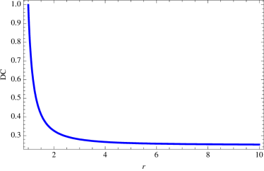
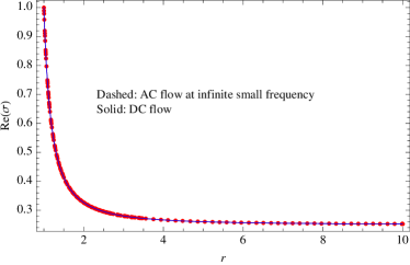
Figure 3: Checking consistency between flows of DC conductivities: Left: Plot of equation (119) from hydrodynamics. Right: comparing the hydrodynamic result and flow equation result. We can see they are explicitly same with each other.

VI Conclusion and Discussion

In this paper, we present a method to work out the RG flows for transport coefficients for quark gluon plasma at finite chemical potential with charged AdS black hole dual. Due to the mixing effect between Maxwell and metric perturbations, we need to solve the coupled equations of motion, which is usually difficult. We organize the system as two coupled Maxwell systems and define two conductivities for each of them. With a parameter characterizing the mixing effect, we write down the mixed flow equations. These mixed RG flow equations will be simplified in certain limits. These flow equations will characterize how the transport coefficients will change as energy scale changes.

We explicitly give the flow equations for conductivity and shear viscosity. In order to check these results analytically we use hydrodynamic method to calculate the Green function at finite cut-off slice $r=r_{c}$. We impose equations of motion at $r=r_{c}$, which is guaranteed by RG invariance of bulk action at classical level Sin:2011yh . Then the Green function can be read off from the on-shell action at $r=r_{c}$. We extended the usual counter term to arbitrary slice in order to have consistent result when $r_{c}\rightarrow\infty$. By using Kubo formula we obtain the analytical results of RG flow formulas for transport coefficients and we found complete agreements with that from flow equations.

Appendix A Derivation of bulk action

Starting from Einstein-Hilbert action, we calculate the bulk action for vector perturbations $a_{z},a_{t},a_{r},A_{x}$ in the 5D RN-AdS background.

$$S=\int d^{5}x\biggr{[}A_{1}a^{\prime}_{t}a^{\prime}_{t}+A_{2}a^{\prime}_{z}a^{\prime}_{z}+DA^{\prime}_{x}A^{\prime}_{x}+Ea_{t}A^{\prime}_{x}\ +\left({\frac{1}{2}}B_{1}a_{t}a_{t}\right)^{\prime}+\left({\frac{1}{2}}B_{2}a_{z}a_{z}\right)^{\prime}+\cdots\biggr{]}.$$ (123)

Here all the prime denotes the $r$ derivative and $\cdots$ represent the terms with $\partial_{t},\partial_{z}$. The coefficients are given by

$$A_{1} = {1\over 2\kappa^{2}}{r^{5}\over 2L^{5}},\quad A_{2}={1\over 2\kappa^{2}}{-fr^{5}\over 2L^{5}}$$ (124)

$$B_{1} = {1\over 2\kappa^{2}}{r^{4}\over L^{5}}\left(-2+{rf^{\prime}\over f}\right),\quad B_{2}={1\over 2\kappa^{2}}{2r^{4}f\over L^{5}}$$ (125)

$$D = {1\over g^{2}}{-r^{3}f\over 2L^{3}},\quad E={1\over g^{2}}{r^{3}{\bar{A}}^{\prime}_{t}\over L^{3}}\ .$$ (126)

Notice that the total derivative terms can be deleted for the purpose of the equations of motion. One can evaluate equations of motion from the action for $a_{t},a_{z},A_{x}$:

$$A_{1}a^{\prime\prime}_{t}+A^{\prime}_{1}a^{\prime}_{t}+EA^{\prime}_{x} = 0$$ (127)

$$A_{2}a^{\prime\prime}_{z}+A^{\prime}_{2}a^{\prime}_{z} = 0$$ (128)

$$(DA^{\prime}_{x}+Ea_{t})^{\prime} = 0.$$ (129)

However we should calculate the final on-shell action by adding proper local counter terms, as we did in section V. We conclude that the mixed bulk action can be written equivalently as two Maxwell actions plus the only mixing term $Ea_{t}A^{\prime}_{x}$.

Appendix B Coefficients for $a_{t}^{\prime}$, $a^{\prime}_{z}$ and $B^{\prime}$

The coefficients for $a_{t}^{\prime}$, $a^{\prime}_{z}$ and $B^{\prime}$ are given by

$$\alpha_{t}(u_{c}) =-u_{c}^{2}g(u_{c})\left[1+b\omega(F_{+1}(u_{c})+F_{-1}(u_{c})))+b^{2}k^{2}(G_{+2}(u_{c})+G_{-2}(u_{c}))\right]+\cdots,$$ (130)

$$\alpha_{z}(u_{c}) =-\frac{\omega}{kf(u_{c})}\alpha_{t}(u_{c})$$ (131)

$$\alpha_{B}(u_{c}) =-\frac{u^{2}g^{\prime}(u_{c})}{2(1+a)}+\frac{bu_{c}^{2}w\left(g(u_{c})\left(F_{-1}^{\prime}(u_{c})-F_{+1}^{\prime}(u_{c})\right)-(F_{-1}(u_{c})+F_{+1}(u_{c}))g^{\prime}(u_{c})\right)}{2(a+1)}$$

$$\quad+\frac{b^{2}k^{2}u_{c}^{2}\left(g(u_{c})\left(G_{-2}^{\prime}(u_{c})-G_{+2}^{\prime}(u_{c})\right)-(G_{-2}(u_{c})+G_{+2}(u_{c}))g^{\prime}(u_{c})\right)}{2(a+1)}$$

$$\quad+\frac{3au_{c}^{2}g^{\prime}(u_{c})b^{2}k^{2}}{4(1+a)^{3}}+\cdots,$$ (132)

$$\beta_{t}(u_{c}) =ib\omega\frac{3au_{c}^{2}g(u_{c})}{f(u_{c})}+\cdots,$$ (133)

$$\beta_{z}(u_{c}) =-\frac{3au_{c}b^{2}k\omega}{2(1+a)}+\cdots,$$ (134)

$$\beta_{B}(u_{c}) =-\frac{3aib\omega}{2(1+a)f(u_{c})}+\cdots.$$ (135)

References

- (1) J. Maldacena, “The large N limit of superconformal field theories and supergravity,” Adv. Theor. Math. Phys. 2, 231 (1998) [Int. J. Theor. Phys. 38, 1113 (1999)] [arXiv:hep-th/9711200]. S. S. Gubser, I. R. Klebanov, and A. M. Polyakov, “Gauge theory correlators from non-critical string theory,” Phys. Lett. B 428, 105 (1998) [arXiv:hep-th/9802109]. E. Witten, “Anti-de Sitter space and holography,” Adv. Theor. Math. Phys. 2, 253 (1998) [arXiv:hep-th/9802150].
- (2) V. Balasubramanian, P. Kraus, A. E. Lawrence and S. P. Trivedi, “Holographic probes of anti-de Sitter space-times,” Phys. Rev. D 59, 104021 (1999) [arXiv:hep-th/9808017]. E. T. Akhmedov, “A Remark on the AdS / CFT correspondence and the renormalization group flow,” Phys.Lett. B442 (1998) 152, [arXiv:hep-th/9806217].
- (3) J. de Boer, E. P. Verlinde and H. L. Verlinde, “On the holographic renormalization group,” JHEP 0008, 003 (2000) [arXiv:hep-th/9912012].
- (4) L. Susskind and E. Witten, “The holographic bound in anti-de Sitter space,” arXiv:hep-th/9805114.
- (5) S. J. Sin and Y. Zhou, JHEP 1105, 030 (2011) [arXiv:1102.4477 [hep-th]].
- (6) I. Heemskerk and J. Polchinski, “Holographic and Wilsonian Renormalization Groups,” arXiv:1010.1264 [hep-th].
- (7) T. Faulkner, H. Liu and M. Rangamani, “Integrating out geometry: Holographic Wilsonian RG and the membrane paradigm,” arXiv:1010.4036 [hep-th].
- (8) I. Bredberg, C. Keeler, V. Lysov and A. Strominger, “Wilsonian Approach to Fluid/Gravity Duality,” arXiv:1006.1902 [hep-th].
- (9) N. Iqbal and H. Liu, “Universality of the hydrodynamic limit in AdS/CFT and the membrane paradigm,” Phys. Rev. D 79, 025023 (2009) [arXiv:0809.3808 [hep-th]].
- (10) M. Parikh and F. Wilczek, Phys. Rev. D 58, 064011 (1998) [arXiv:gr-qc/9712077].
- (11) K. G. Wilson and J. B. Kogut, “The Renormalization group and the epsilon expansion,” Phys. Rept. 12 (1974) 75–200. K. G. Wilson, “The renormalization group and critical phenomena,” Rev. Mod. Phys. 55 (1983) 583–600. F. J. Wegner and A. Houghton, “Renormalization group equation for critical phenomena,” Phys.Rev. A8 (1973) 401–412. J. Polchinski, “Renormalization and Effective Lagrangians,” Nucl. Phys. B231 (1984) 269–295.
- (12) T. Faulkner, H. Liu, J. McGreevy and D. Vegh, “Emergent quantum criticality, Fermi surfaces, and AdS2,” arXiv:0907.2694 [hep-th].
- (13) T. Faulkner and J. Polchinski, “Semi-Holographic Fermi Liquids,” arXiv:1001.5049 [hep-th].
- (14) G. Policastro, D. T. Son and A. O. Starinets, “From AdS/CFT correspondence to hydrodynamics,” JHEP 0209, 043 (2002) [arXiv:hep-th/0205052].
- (15) H. Kodama, A. Ishibashi and O. Seto, Phys. Rev. D 62, 064022 (2000) [arXiv:hep-th/0004160].
- (16) P. K. Kovtun and A. O. Starinets, Phys. Rev. D 72, 086009 (2005) [arXiv:hep-th/0506184].
- (17) P. Kovtun, D. T. Son and A. O. Starinets, “Holography and hydrodynamics: Diffusion on stretched horizons,” JHEP 0310, 064 (2003) [arXiv:hep-th/0309213].
- (18) D. Nickel and D. T. Son, “Deconstructing holographic liquids,” arXiv:1009.3094 [hep-th].
- (19) S. A. Hartnoll, Class. Quant. Grav. 26, 224002 (2009) [arXiv:0903.3246 [hep-th]].
- (20) D. T. Son and A. O. Starinets, “Minkowski-space correlators in AdS/CFT correspondence: Recipe and applications,” JHEP 0209, 042 (2002) [arXiv:hep-th/0205051].
- (21) X. H. Ge, Y. Matsuo, F. W. Shu, S. J. Sin and T. Tsukioka, Prog. Theor. Phys. 120, 833 (2008) [arXiv:0806.4460 [hep-th]].
- (22) M. Edalati, J. I. Jottar and R. G. Leigh, JHEP 1004, 075 (2010) [arXiv:1001.0779 [hep-th]].
- (23) E. Witten, “Multi-trace operators, boundary conditions, and AdS/CFT correspondence,” arXiv:hep-th/0112258. M. Berkooz, A. Sever and A. Shomer, “Double-trace deformations, boundary conditions and spacetime singularities,” JHEP 0205, 034 (2002) [arXiv:hep-th/0112264]. W. Mueck, “An improved correspondence formula for AdS/CFT with multi-trace operators,” Phys. Lett. B 531, 301 (2002) [arXiv:hep-th/0201100]. P. Minces, “Multi-trace operators and the generalized AdS/CFT prescription,” Phys. Rev. D 68, 024027 (2003) [arXiv:hep-th/0201172].
- (24) L. Vecchi, “Multitrace deformations, Gamow states, and Stability of AdS/CFT,” arXiv:1005.4921 [hep-th]. A. Sever and A. Shomer, “A note on multi-trace deformations and AdS/CFT,” JHEP 0207, 027 (2002) [arXiv:hep-th/0203168]. M. Li, “A note on relation between holographic RG equation and Polchinski’s RG equation,” Nucl. Phys. B 579, 525 (2000) [arXiv:hep-th/0001193]. A. C. Petkou, “Boundary multi-trace deformations and OPEs in AdS/CFT correspondence,” JHEP 0206, 009 (2002) [arXiv:hep-th/0201258]; E. T. Akhmedov, “Notes on multi-trace operators and holographic renormalization group,” arXiv:hep-th/0202055;
- (25) H. Kodama and A. Ishibashi, Prog. Theor. Phys. 111 (2004) 29 [arXiv:hep-th/0308128].
- (26) V. Balasubramanian and P. Kraus, Commun. Math. Phys. 208 (1999) 413 [arXiv:hep-th/9902121].