Dynamic Voids Surrounded by Shocked
Conventional Polytropic Gas Envelopes

Abstract

With proper physical mechanisms of energy and momentum input from around the centre of a self-gravitating polytropic gas sphere, a central spherical “void” or “cavity” or “bubble” of very much less mass contents may emerge and then dynamically expand into a variety of surrounding more massive gas envelopes with or without shocks. We explore self-similar evolution of a self-gravitating polytropic hydrodynamic flow of spherical symmetry with such an expanding “void” embedded around the center. The void boundary supporting a massive envelope represents a pressure-balanced contact discontinuity where drastic changes in mass density and temperature occur. We obtain numerical void solutions that can cross the sonic critical surface either smoothly or by shocks. Using the conventional polytropic equation of state, we construct global void solutions with shocks travelling into various envelopes including static polytropic sphere, outflow, inflow, breeze and contraction types. In the context of supernovae, we discuss the possible scenario of separating a central collapsing compact object from an outgoing gas envelope with a powerful void in dynamic expansion. Initially, a central bubble is carved out by an extremely powerful neutrinosphere. After the escape of neutrinos during the decoupling, the strong electromagnetic radiation field and/or electron-positron pair plasma continue to drive the cavity expansion. In a self-similar dynamic evolution, the pressure across the contact discontinuity decreases with time to a negligible level for a sufficiently long lapse and eventually, the gas envelope continues to expand by inertia. We describe model cases of polytropic index $\gamma=4/3-\epsilon$ with $\epsilon>0$ and discuss pertinent requirements to justify our proposed scenario.

1 Introduction

Voids of much less density as compared to more massive and grossly spherical surroundings are fairly common in astrophysical systems on various spatial and temporal scales. They have been found in a wide diversity of settings, including planetary nebulae (PNe) (e.g. NGC 7662 and NGC 40; Guerrero et al., 2004, Lou & Zhai 2010), bubbles and superbubbles (e.g. McCray & Kafatos, 1987; Korpi et al., 1999) in the interstellar medium (ISM), supernovae (SNe), supernova remnants (SNRs) and so forth. It is conceivable that with sustained powerful sources of energy and momentum released from around the central region of a self-gravitating gas sphere, a considerably rarified void or cavity or bubble can form and dynamically expand into a more massive surrounding envelope. Depending astrophysical contexts, such sustained central sources could be tenuous stellar winds, magnetized relativistic pulsar winds of mainly electron-positron pair plasma, energetic neutrino flux, and radiation field of trapped photon gas etc. We advance in this paper a theoretical model scenario, which is formulated within the framework of self-similar evolution for a conventional polytropic gas, towards general profiles of spherically symmetric hydrodynamic systems embedded with central voids in expansion. As a simplifying approximation, these voids are treated as massless quasi-spherical cavities whose gravitational fields are negligible when considering the dynamic evolution of the gas shells surrounding the central voids. Naturally, there are always some materials inside the boundary of any void in reality. They are even indispensable for explaining the dynamic evolution of the shell outside in aspects other than gravity (e.g., pressure driving, tenuous wind driving, extremely relativistic light particles, and photon gas etc.). With these qualifications in mind, our analysis would indicate that this model is capable and applicable for describing a variety of polytropic gaseous astrophysical envelopes in hydrodynamic evolution. Some similar analysis along this line can be found in (Lou & Zhai, 2009, 2010), which focus on isothermal cases (i.e. isothermal self-similar voids – ISSV) and astrophysical applications to PNe NGC 40 and NGC 7662 as examples; such central ISSV in PNe are powered by hot tenuous stellar winds with shocks.

Originated from extremely violent processes like supernova explosions, “hot bubbles” or voids filled with intense radiation fields are a significant kind of structures in the evolution of many astrophysical systems including supernova remnants (SNRs). One of our main concerns here is on various void structures in the self-similar dynamic evolution of SNe and subsequent SNRs. Matzner & McKee (1999) noted the existence of similarities in the evolution of SNe at a very early epoch – much earlier than the Sedov stage known for its characteristics of self-similar evolution. It would be a first approximation to investigate dynamic evolution of SNe, whose mass is sufficiently large ($\;\lower 4.0pt\hbox{${\buildrel\displaystyle>\over{\sim}}$}\;8M_{\odot}$) as compared with the mass of the central collapsed compact object ($\sim 1.5M_{\odot}$), by self-similar hydrodynamic models with central voids.

Formation of such initial “voids” within one or two hundred kilometers is plausibly the result of intense neutrino flux heating and driving, leading to the emergence of a rebound shock. This Wilson mechanism was put forward and elaborated by Bethe & Wilson (1985) (and subsequently in Bethe, 1990), where the authors argued that acceleration of mass infall towards the center is inhibited by the neutrino pressure from the so-called neutrinosphere with little amount of mass. This mechanism is highlighted in numerical simulations of Janka & Hillebrandt (1989b) and Janka & Müller (1996) for examples. These simulation works have sketched a picture by simulation that stellar materials are heated and pushed outwards by the intense neutrino flux generated by nuclear processes during the rapid core collapse at the centre. As a by-product of rebound shock revitalization, a bubble or cavity will have already been shaped up around the center during the epoch before the surrounding gas materials become too tenuous ($\sim 10^{9}\mbox{ g }\mbox{cm}^{-3}$ as discussed presently in subsection 4.3) to trap extremely energetic neutrinos. Then the envelope shell, consisting of the vast majority of stellar materials, is expected to be ejected by the revived rebound shock. After a short while, relativistic neutrinos and outer surrounding massive gas envelope becomes completely decoupled.

We further discuss this physical feasibility regarding two factors: energy and momentum transfers from photons to an ionized plasma are very effective (compared with that from neutrinos to gas); the energy carried by radiative emissions of photons is of the same order of magnitude ($\sim 10^{51}\mbox{ erg}$) as the energy needed to blow a stellar envelope up. Our dynamic void solutions show that it could be the photon radiation field trapped inside the central cavity that drives an outer shell to expand after the decoupling and escape of energetic neutrinos. As simplifications, we would treat a void containing a uniform radiation field instead of a mixture of conventional matters and radiation coupled by transport equations. The scale of a central void at the very early stage ($\;\lower 4.0pt\hbox{${\buildrel\displaystyle>\over{\sim}}$}\;100\mbox{ km}$, e.g. Bethe, 1990) makes this uniformity approximation plausible as the perturbation in radiation field travels at the speed of light $c$. Here the concept of radiation field is usually generalized as a combination of photons (electromagnetic field) and various products of pair-production such as electron-positron pairs, since the temperatures are always sufficiently high (at least $k_{\text{B}}T>1\mbox{ MeV}$) for pair production, where $k_{B}$ is the Boltzmann constant. This radiation-driven envelope expansion with self-gravity is then responsible for the acceleration and/or deceleration in the expansion of a SN; we shall come back to this possibility later in this paper.

We conduct in this paper a systematic analysis of the self-similar hydrodynamic evolution of void surrounded by spherical envelopes with various radial structures using the similarity transformation. Self-similar hydrodynamics with spherical symmetry has been extensively studied as a valuable tool with various approximations and simplifications. The research works of Larson (1969a, b), Penston (1969a, b), Hunter (1977, 1986), Shu (1977), Tsai & Hsu (1995), Chevalier (1997), Shu et al. (2002), Lou & Shen (2004), Shen & Lou (2004), and Bian & Lou (2005), have investigated self-similar hydrodynamics and their astrophysical applications with an isothermal equation of state (EoS). Meanwhile, those with polytropic EoS have been studied by Goldreich & Weber (1980), Yahil (1983), Lattimer et al. (1985), Suto & Silk (1988), Lou & Wang (2006), Hu & Lou (2008), and Lou & Cao (2008). Some of them are more pertinent to our investigation here, e.g. Hunter (1977) obtained a systematic self-similar transformation and obtained the isothermal expansion-wave collapse solution (EWCS), which has been substantially generalized; Tsai & Hsu (1995) introduced a procedure of treating shocks in an isothermal gas; Yahil (1983) and Suto & Silk (1988) developed self-similar procedure for conventional polytropic gas dynamics; Lou & Wang (2006) and Lou & Cao (2008) explored the scheme for the evolution of conventional and general polytropic gases with shocks. Self-similar transformations permit a series of central-void solutions (Lou & Zhai 2009, 2010 for isothermal cases and Hu & Lou 2008 for polytropic voids as examples) whose boundaries appear to be very steep in mass density. This treatment is again an idealization and the justification of doing so is discussed in Appendix D. We are also interested in the construction of self-similar conventional polytropic shock solutions with expanding central voids.

We note Yahil (1983) and Lou & Cao (2008) for their analyses of cases whose polytropic indices are $\gamma\rightarrow(4/3)^{+}$ and $\gamma=4/3$. For either relativistically hot or degenerate materials, it is a very good approximation to describe their behaviour by an adiabatic EoS $p=\kappa\rho^{4/3}$. Here $\kappa$ is a function of $(r,\ t)$ in general polytropic cases satisfying specific entropy conservation along streamlines (e.g. Fatuzzo et al., 2004). Specification of $\kappa$ as a global constant is a special case, i.e., a conventional polytropic gas. An exact $\gamma=4/3$ case is analyzed by Goldreich & Weber (1980) for a homologous core collapse solution. In this paper, we emphasize void solutions with conventional polytropic conditions whose $\gamma$ takes the form of $\gamma=4/3-\epsilon$ with a small $\epsilon>0$ and discuss the physical implication of $\epsilon$. We propose possible situations to sustain such void expansions in astrophysical contexts.

This paper is structured as follows. Section 1 introduces background information, the physical problem, and our research motivation. In Section 2, we show and discuss the formulation of self-similar transformation of hydrodynamic equations, as well as solution behaviours near sonic critical points and shock jump conditions. Section 3 discusses the behaviours of solutions near the void boundaries and gives various conventional polytropic self-similar void solutions crossing the sonic critical surface by different manners; shock solutions with different kinds of dynamic envelopes are presented. We shall explore applications of those models especially in the context of SN in Section 4 and some examples are presented there. Section 5 contains conclusions and related discussions. Appendices A to E offer details of physical reasoning and some mathematical derivations.

2 Formulation of Self-similar Model

We first present below the nonlinear Euler hydrodynamic partial differential equations (PDEs) with spherical symmetry and self-gravity. In spherical polar coordinates in which a spatial point is defined by $(r,\ \theta,\ \phi)$ where $r$ is the radius, $\theta$ is the polar angle and $\phi$ is the azimuthal angle, we will introduce self-similar transformation for a conventional polytropic gas (e.g. Suto & Silk, 1988; Hu & Lou, 2008). For spherically symmetric hydrodynamics, all the dependent physical variables do not vary with angles $\theta$ and $\phi$.

2.1 Euler hydrodynamic PDEs, conventional polytropic self-similar transformation,
    and asymptotic solutions

With spherical symmetry and self-gravity, we have the radial momentum equation as

$$\dfrac{\partial u}{\partial t}+u\dfrac{\partial u}{\partial r}=-\dfrac{1}{\rho}\dfrac{\partial p}{\partial r}-\dfrac{GM}{r^{2}}\ ,$$ (1)

where we use $u$ to denote the radial flow velocity, $t$ for the time, $p$ for the pressure, $\rho$ for the mass density, $M$ for the enclosed mass within radius $r$ at time $t$, and $G=6.67\times 10^{-8}\mbox{ dyn }\mbox{cm}^{2}\mbox{ g}^{-2}$ for the universal gravitational constant. Nonlinear PDE (1) is coupled with the mass conservation

$$\dfrac{\partial\rho}{\partial t}+\dfrac{1}{r^{2}}\dfrac{\partial}{\partial r}\left(\rho ur^{2}\right)=0\ ,$$ (2)

or equivalently, in the integral form of

$$\begin{split}&\dfrac{\partial M}{\partial t}+u\dfrac{\partial M}{\partial r}=0\ ,\\ &\dfrac{\partial M}{\partial r}=4\pi r^{2}\rho\ .\end{split}$$ (3)

A closed set of nonlinear PDEs is established when we include the conventional polytropic EoS,

$$p=\kappa\rho^{\gamma}\ ,$$ (4)

where $\gamma$ is a constant index and $\kappa$ is a global constant.

A self-similar transformation based on dimensional analysis [e.g. Suto & Silk (1988)] for a conventional polytropic gas is introduced below, namely

$$\begin{split}&x=\dfrac{r}{k^{1/2}t^{n}}\ ,\quad u(r,t)=k^{1/2}t^{n-1}v(x)\ ,\quad\rho(r,t)=\dfrac{\alpha(x)}{4\pi Gt^{2}}\ ,\\ &p(r,\ t)=\dfrac{kt^{2n-4}}{4\pi G}[\alpha(x)]^{\gamma},\quad M(r,\ t)=\dfrac{k^{3/2}t^{3n-2}}{(3n-2)G}m(x)\ ,\end{split}$$ (5)

where $k$ is the sound parameter and $n$ is the scaling exponent, $x$ is the dimensionless independent similarity variable, and depending on $x$ only, $v(x)$, $\alpha(x)$ and $m(x)$ are the dimensionless reduced variables for radial flow velocity $u(r,\ t)$, mass density $\rho(r,\ t)$ and enclosed mass $M(r,\ t)$, respectively. Under transformation (5), nonlinear PDEs (1) to (4) are converted into two coupled nonlinear ordinary differential equations (ODEs), viz.,

$$\begin{split}&\dfrac{\mbox{d}\alpha}{\mbox{d}x}=\dfrac{\alpha}{(nx-v)^{2}-\gamma\alpha^{\gamma-1}}\\ &\ \times\left[(n-1)v+\dfrac{(nx-v)}{(3n-2)}\alpha-2\dfrac{(x-v)(nx-v)}{x}\right],\\ &\dfrac{\mbox{d}v}{\mbox{d}x}=\dfrac{1}{(nx-v)^{2}-\gamma\alpha^{\gamma-1}}\\ &\times\left[(nx-v)(n-1)v+\dfrac{(nx-v)^{2}}{(3n-2)}\alpha-2\gamma\dfrac{x-v}{x}\alpha^{\gamma-1}\right].\end{split}$$ (6)

According to Suto & Silk (1988), the conventional polytropic condition for a time-independent $\kappa$ in polytropic relation (4) simply requires $n+\gamma=2$.

With $n+\gamma=2$ and the assumption that $|v(x)|$ and $\alpha(x)$ are non-increasing functions of $x$ at very large $x$, $v(x)$ and $\alpha(x)$ have the following asymptotic behaviours in the regime $x\gg 1$, namely

$$\begin{split}\alpha&=Ax^{-2/n}\ ,\\ v&=Ax^{(n-2)/n}\left[\dfrac{2(2-n)}{nA^{n}}-\dfrac{n}{(3n-2)}\right]\\ &\qquad\qquad-\dfrac{(n-1)}{n}B^{2}x^{(n-2)/n}+Bx^{(n-1)/n}\end{split}$$ (7)

(Lou & Shi 2011 in preparation), where $A$ and $B$ referred to as mass and speed parameters are two integration constants, characterizing asymptotic behaviours at large $x$.

The isothermal case of $n=1$ and $B=0$ was studied by Shu (1977), and a generalization of $B\neq 0$ for an isothermal gas was pursued by Whitworth & Summers (1985) for solutions with weak discontinuities (Lou & Shen 2004).

Clearly, for all $n>0$ and $B\neq 0$, $Bx^{(n-1)/n}$ is the leading term in the asymptotic solution of $v(x)$ for large $x$. Specific for isothermal cases (i.e. $n=1$ and $\gamma=1$), $B$ actually represents the constant reduced speed at $x\rightarrow+\infty$ (e.g. Lou & Shen, 2004). In reference to our previous work (e.g. Lou & Wang, 2006), we shall refer to solutions according to their large$-x$ asymptotic envelope behaviours as follows in this paper: $B=0$ and $v>0$ for “breeze solutions”; $B=0$ and $v<0$ for “contraction solutions”; $B>0$ (thus $v>0$ for large enough $x$) for “outflow solutions”; $B<0$ (thus $v<0$ for large enough $x$) for “inflow solutions”.

Similarity transformation (5) and hydrodynamic PDEs lead to the following algebraic relation

$$m=\alpha x^{2}(nx-v)\ ,$$ (8)

which implies the presence of the so-called “zero-mass line” (ZML) specified by $nx-v=0$ in the $-v(x)$ versus $x$ figure presentation; below this ZML a negative enclosed mass $M(r,\ t)$ would be physically unacceptable.

2.2 The sonic critical curve and eigensolutions

In two coupled nonlinear hydrodynamic ODEs (6), we encounter a sonic critical point when the denominators on the right-hand side (RHS) vanish (Suto & Silk, 1988, n.b. $n+\gamma=2$), i.e.

$$nx-v=(2-n)^{1/2}\alpha^{(1-n)/2}\ .$$ (9)

In the three-dimensional (3D) variable space of $x$, $v$ and $\alpha$, condition (9) represents a two-dimensional (2D) surface of singularity for two coupled nonlinear ODEs (6). In general, a solution cannot go across this surface smoothly due to the singularity of ODEs except for a special type of solutions, viz., the eigensolutions. One important necessary condition for searching such eigensolutions is that the numerators on the RHS also vanish simultaneously, which is equivalent to (see also Suto & Silk, 1988)

$$(n-1)v+\dfrac{(nx-v)}{(3n-2)}\alpha-2\dfrac{(x-v)(nx-v)}{x}=0\ .$$ (10)

While requirement (10) is derived to have the numerator of $\mbox{d}\alpha/\mbox{d}x$ to vanish, it is straightforward to verify that the numerator of $\mbox{d}v/\mbox{d}x$ in eq. (6) also vanishes with eq. (9) given (see Suto & Silk, 1988, Lou & Shi 2011 in preparation). In other words, conditions (9) and (10) are sufficient to determine those eigensolutions crossing the sonic critical curve (SCC) smoothly, leaving one degree of freedom (DOF), i.e. the specific point at which the eigensolutions go across. ODEs (9) and (10) are combined to determine the SCC in the 3D variable space of $x$, $v$ and $\alpha$. The points at which the eigensolutions cross the critical surface smoothly are all located along the SCC. In the following, we shall use $x_{0}$, $v_{0}$ and $\alpha_{0}$ to denote values of $x$, $v$ and $\alpha$ on the SCC for solutions crossing the SCC smoothly. When solving two ODEs (9) and (10) explicitly for $x_{0}$, $v_{0}$ and $\alpha_{0}$, we find that the SCC consists of two segments represented by subscripts $+$ and $-$ respectively as two connected quadratic solutions:

$$\begin{split}x_{0,\pm}&=\dfrac{-K_{b}\pm(K_{b}^{2}-4K_{a}K_{c})^{1/2}}{2K_{a}}\ ,\\ v_{0,\pm}&=nx_{0,\pm}-(2-n)^{1/2}\alpha_{0}^{(1-n)/2}\ ,\end{split}$$ (11)

where

$$\begin{split}K_{a}&\equiv n(n-1)\ ,\\ K_{b}&\equiv(2-n)^{1/2}\left(n-1+\dfrac{\alpha_{0}}{3n-2}\right)\alpha_{0}^{(1-n)/2}\ ,\\ K_{c}&\equiv 2(n-2)\alpha_{0}^{1-n}\end{split}$$ (12)

(Lou & Cao, 2008). These two $+$ and $-$ segments of the SCC meet right at the point where

$$\alpha_{0}=-3n^{2}+5n-2+2\big{[}2(4n-16n^{2}+21n^{3}-9n^{4})\big{]}^{1/2}.$$ (13)

We combine these two SCC branches to form a smooth global SCC. In the following, we refer to the segment with “$+$” in eq. (11) as segment 1, while that with “$-$” in eq. (11) as segment 2, respectively.

We then expand an eigensolution to the first order near the SCC as

$$x=x_{0}+\delta\ ,\qquad\alpha=\alpha_{0}+\alpha^{\prime}\delta\ ,\qquad v=v_{0}+v^{\prime}\delta\ ,$$ (14)

where $\alpha^{\prime}$ and $v^{\prime}$ are the values of $\mbox{d}\alpha/\mbox{d}x$ and $\mbox{d}v/\mbox{d}x$ on the SCC for eigensolutions, respectively. Solving two ODEs (9) and (10), we obtain a quadratic equation of $v^{\prime}$ as well as the equation of $\alpha^{\prime}$ (see also Suto & Silk, 1988):

$$av^{\prime 2}+bv^{\prime}+d=0\ ,\quad\alpha^{\prime}=\dfrac{\alpha_{0}^{(n+1)/2}}{(2-n)^{1/2}}\left(v^{\prime}-2\dfrac{x_{0}-v_{0}}{x_{0}}\right),$$ (15)

where three coefficients $a$, $b$ and $c$ are explicitly defined by

$$\begin{split}a&\equiv 3-n\ ,\\ b&\equiv 4(1-n)\dfrac{v_{0}}{x_{0}}+5n-7\ ,\\ d&\equiv 2(3-2n)\dfrac{v_{0}^{2}}{x_{0}^{2}}+2\left(\dfrac{\alpha_{0}}{3n-2}+2n-4\right)\dfrac{v_{0}}{x_{0}}\\ &\qquad\qquad\qquad\qquad+\dfrac{(n-2)}{(3n-2)}\alpha_{0}-2n+4\ .\end{split}$$ (16)

Quadratic equation (15) for $v^{\prime}$ generally allows two roots, corresponding to two types of possible eigensolutions across the SCC at the same point on the SCC (Lou & Cao, 2008). To be specific, with the formula of roots of quadratic equation (15), we obtain the two roots of $v^{\prime}$ explicitly as

$$v^{\prime}_{\pm}=\dfrac{-b\pm(b^{2}-4ad)^{1/2}}{2a}\ .$$ (17)

For an eigensolution crossing the SCC only once, those with $v^{\prime}_{-}$ will be referred to as type-1 solutions while those with $v^{\prime}_{+}$ are type-2 solutions. In general, those sonic critical points at which the solution take $v^{\prime}=v^{\prime}_{-}$ will be referred to as type-1 critical point, while $v^{\prime}=v^{\prime}_{+}$ for type-2 critical point.

2.3 Shock jump conditions across the SCC

For astrophysical applications, it is common to expect the existence of shocks in the hydrodynamic evolution of a gas sphere. Across a shock front propagating in a conventional polytropic gas, conditions of the mass conservation

$$(\rho_{2}-\rho_{1})u_{s}=u_{2}\rho_{2}-u_{1}\rho_{1}\ ,$$ (18)

the radial momentum conservation

$$u_{s}(u_{2}\rho_{2}-u_{1}\rho_{1})=-p_{1}+p_{2}-u_{1}^{2}\rho_{1}+u_{2}^{2}\rho_{2}\ ,$$ (19)

and the energy conservation

$$\begin{split}&u_{s}\left(-\dfrac{p_{1}}{\gamma-1}+\dfrac{p_{2}}{\gamma-1}-\frac{u_{1}^{2}\rho_{1}}{2}+\frac{u_{2}^{2}\rho_{2}}{2}\right)\\ &=u_{2}\left(\dfrac{\gamma p_{2}}{\gamma-1}+\frac{u_{2}^{2}\rho_{2}}{2}\right)-u_{1}\left(\dfrac{\gamma p_{1}}{\gamma-1}+\frac{u_{1}^{2}\rho_{1}}{2}\right)\ ,\end{split}$$ (20)

need to be satisfied in the co-moving shock reference framework in order to attain a physically acceptable shock discontinuity. We note here, especially for the energy conservation across the shock front, that the polytropic index $\gamma$ should remain the same across a shock front for similarity solutions; if those $\gamma$ are different, $n$ would be also different because of $n+\gamma=2$. This would not be acceptable for a global similarity evolution in which a shock evolves self-similarly.

It is useful to point out that those three shock equations above are invariant under a commutation of subscripts 1 and 2. We need to know the direction for entropy increase for identifying physical shock solutions. To be specific, we denote subscript 1 for the upstream flow. Solving combined shock conditions (18)$-$(20) and adopting self-similar transformation (5), those conservation conditions become explicitly ($x_{\text{s1}}$ is the self-similar location of the shock on the upstream side and $x_{\text{s2}}$ being that of the downstream side; in fact, they correspond to the same shock radius $r_{s}(t)$ but with different $k$ values for the sound parameter)

$$\begin{split}&\alpha_{2}=\frac{\alpha_{1}^{2}(\gamma+1)\left(v_{1}-nx_{\text{s1}}\right)^{2}}{\alpha_{1}(\gamma-1)\left(v_{1}-nx_{\text{s1}}\right)^{2}+2\gamma\alpha_{1}^{\gamma}}\ ,\\ &x_{s2}=x_{s1}\bigg{[}\dfrac{\alpha_{2}^{\gamma}(\gamma+1)}{2(v-nx_{s1})^{2}-\alpha_{1}^{\gamma}(\gamma-1)}\bigg{]}^{1/2}\ ,\\ &v_{2}=\dfrac{2nx_{s1}+v_{1}(\gamma-1)+\dfrac{2\gamma\alpha_{1}^{\gamma-1}}{(v_{1}-x_{s1})}}{(\gamma+1)}\dfrac{x_{s2}}{x_{s1}}\ ,\end{split}$$ (21)

which are sufficient to determine those important self-similar variables {$x$, $v$, $\alpha$} at the immediate downstream side of a shock front when those of the immediate upstream side are known. The other way around, it is also straightforward to determine physical variables of the upstream side when physical variables of the downstream side are specified.

In addition, we introduce parameter $\eta_{k}$ for convenience as the ratio of different sound parameter $k$ values at the upstream to downstream sides across a shock front, namely

$$\eta_{k}=\dfrac{k_{1}}{k_{2}}=\left(\dfrac{x_{s2}}{x_{s1}}\right)^{2}=\dfrac{\alpha_{2}^{\gamma}(\gamma+1)}{2(v-nx_{s1})^{2}-\alpha_{1}^{\gamma}(\gamma-1)}\ .$$ (22)

Apparently, $\eta_{k}$ reflects the strength of an expanding shock in a self-similar dynamic evolution.

This $\eta_{k}$ parameter here is equivalent to $1/\lambda$ in the formulation of Lou & Wang (2006). We now discuss the variation of specific entropy along streamlines, reflected by the variation of $k$ (or $\kappa$; $\kappa=k(4\pi G)^{\gamma-1}t^{2(n+\gamma-2)}$ for a general polytropic gas and $\kappa=k(4\pi G)^{1-n}$ for a conventional polytropic gas) across an outgoing shock front. The Mach number $\mathcal{M}_{i}$ of a shock is defined by

$$\mathcal{M}_{i}=|u_{s}-u_{i}|/s_{i}\ ,$$ (23)

where $i=1,\ 2$ refer to immediate upstream and downstream sides, respectively, and $u_{i}$ is the radial flow speed near the shock front, $s_{i}$ is the sound speed, $u_{s}$ is the expansion speed of the shock front in our frame of reference. Using similarity transformation (5), we derive the Mach number of a shock in self-similar form on either side of a shock front as

$$\mathcal{M}_{i}=\dfrac{x_{i}^{2}}{\gamma\alpha_{i}^{\gamma-1}}\Gamma_{i}\ ,$$ (24)

where notations $\Gamma_{i}$ and $z$ are defined by

$$\Gamma_{i}\equiv n-v_{i}/x_{i}\ ,\qquad\quad z\equiv\Gamma_{2}/\Gamma_{1}\ ,$$ (25)

which are the same as those in Lou & Wang (2006). In the following discussion, we assume $\gamma>1$. It is then straightforward to show that when $\mathcal{M}_{1}>1$, we must have $z<1$. Since $z<1$ gives (see also Lou & Wang 2006)

$$\dfrac{\mbox{d}(\lambda^{2})}{\mbox{d}z}=\dfrac{\mbox{d}}{\mbox{d}z}\bigg{(}\dfrac{1}{\eta_{k}^{2}}\bigg{)}=-\dfrac{\gamma(\gamma^{2}-1)(z-1)^{2}z^{\gamma-1}}{\left[(\gamma+1)z-(\gamma-1)\right]^{2}}<0\ ,$$ (26)

and $\lambda\rightarrow 1$ when $z\rightarrow 1$, this derivation yields that when $\mathcal{M}_{1}>1$, inequalities $\lambda>1$ and $\eta_{k}<1$ (thus $k_{1}<k_{2}$ and $\kappa_{1}<\kappa_{2}$) will hold. This indicates the fact that the shock wave is supersonic in the upstream flow ($\mathcal{M}_{1}>1$) and causes an increase of entropy across a shock front (i.e., $\kappa_{2}>\kappa_{1}$). If however $\mathcal{M}_{1}$ is less than $1$, subscript $1$ would therefore denote downstream and the condition of entropy increase still holds (i.e., $\kappa_{2}<\kappa_{1}$). In summary, shock jump conditions (18)$-$(20) and naturally their solutions (21) are invariant with respect to a commutation of subscripts $1$ and $2$; the irreversibility of a shock or the increase of specific entropy across a shock front should not be violated.

3 Conventional Polytropic Self-similar Void Solutions

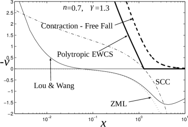
Figure 1: Examples of conventional polytropic self-similar solutions (Lou & Wang, 2006). These solutions have $n=0.7$ (thus $\gamma=1.3$). For a clearer illustration, the horizontal $x$-axis is shown in a logarithmic scale. The dash-dotted curve is the SCC, shown as a reference here. The light solid curve marked by “Lou & Wang” is the solution that crosses the SCC twice. It has two critical points on the SCC at $(\alpha,\ x,\ v)=(164.69,\ 0.002978,\ -2.4497)$ for a type-2 crossing and $(\alpha,\ x,\ v)=(0.1639,\ 3.4684,\ 1.5586)$ for a type-1 crossing, respectively (see Lou & Wang (2006) for more details). The heavy dashed curve marked by “Contraction - Free Fall” is the solution with contraction envelope and a free-fall collapsing core with asymptotic behaviour $A=A_{\text{e}}+0.3$ ($A_{\text{e}}$ is given by eq. (28)), a polytropic counterpart of similar isothermal results in Shu (1977). The heavy solid curve is the polytropic EWCS solution ($A\rightarrow A_{\text{e}}^{+}$). The dotted curve is the zero-mass line (ZML with $nx=v$).

3.1 Several pertinent self-similar solutions presented in Lou & Wang (2006) and
   Lou & Cao (2008)

We first illustrate here several related self-similar solutions for conventional polytropic gas flows already obtained earlier. These are important in two aspects, viz., validating our numerical code and preparing for further model analysis for self-similar voids surrounded by various dynamic envelopes.

3.1.1 Conventional polytropic expansion-wave
   collapse solution (EWCS)

Expansion-wave collapse solutions (EWCSs) were studied originally in an isothermal gas by Shu (1977). The natural generalization to conventional polytropic EoS was done by Cheng (1978). With a general polytropic EoS, this kind of solutions with $\gamma=4/3$ and $n+\gamma\neq 2$ has been constructed by Lou & Cao (2008) in recent years.

Conditions for EWCS can be readily derived from self-similar hydrodynamic ODE (6); meanwhile, those for the outer portion of a static envelope of a singular polytropic sphere (SPS) have been constructed (e.g. Lou & Wang, 2006). We can independently use some practical methods to obtain these solutions numerically with asymptotic solutions (7) in the regime of large $x$. As the coefficient of the leading term in the asymptotic expression of $v(x)$, speed parameter $B$ must vanish for this type of solution for a static polytropic envelope. For mass parameter $A$, we can get it from the asymptotic solution of $v(x)$ by making the coefficient of the term of order $x^{(n-2)/n}$ to vanish, i.e.

$$\left[\dfrac{2(2-n)}{nA^{n}}-\dfrac{n}{(3n-2)}\right]\rightarrow 0^{-}\ ,$$ (27)

which then yields ($A_{\text{e}}$ is the limit for mass parameter $A$ to achieve the conventional polytropic EWCS)

$$A\rightarrow A_{\text{e}}^{+}\ ,\qquad\qquad A_{\text{e}}=\left[\dfrac{2(2-n)(3n-2)}{n^{2}}\right]^{1/n}\ .$$ (28)

For the isothermal EWCS of Shu (1977), we have $n=1$ and $A_{\text{e}}=2$. This $A_{\text{e}}$ value of $A$ represents a limit. An exact equality of $A=A_{\text{e}}$ would correspond to the SPS solution.

EWCS can be regarded as a special case bounding “collapse solutions without critical points” with $A>A_{\text{e}}$ (e.g. Shu, 1977; Lou & Zhai, 2009). Here we present one of such solutions with $n=0.7$ in Fig. 1 (the conventional polytropic relation $n+\gamma=2$ holds). We found that the behaviours of solutions are qualitatively similar to isothermal cases as $A$ gradually goes down to $A_{\text{e}}=2$ (see Lou & Cao, 2008); here the limit of $A$ becomes $A_{\text{e}}=0.4044$ for $n=0.7$. For an exact conventional polytropic EWCS, a discontinuity in the first derivative appears at $x=1.3085$, where the central infall side solution is tangent to the SCC. This discontinuity in first derivatives denotes the front of an expansion wave in self-similar evolution inside of which a collapse takes place and beyond which the gas remains a static conventional polytropic envelope (i.e. outer part of a SPS). We shall further construct this kind of solutions in the following.

3.1.2 Solutions crossing the SCC smoothly

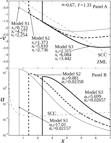
Figure 2: Conventional polytropic void solutions crossing the SCC smoothly with $n=0.67$ (thus $\gamma=1.33$). Panel A illustrates the profiles of negative reduced radial speed $-v(x)$ versus $x$ and Panel B shows the corresponding profiles of reduced mass density $\alpha(x)$ versus $x$ where the $\alpha$-axis is in the logarithmic scale. The dash-dotted curves in both panels are the SCCs, while the light dotted line in Panel A is the ZML. Three solutions of such type, marked by Model S1 to S3 (S for “smooth”) are plotted in light solid curve, heavy dashed curve and heavy solid curve, respectively. Model S1 crosses the SCC at $(x_{0},\ v_{0},\ \alpha_{0})=(4.277,\ 2.254,\ 0.02157)$, Model S2 at $(x_{0},\ v_{0},\ \alpha_{0})=(5.010,\ 2.736,\ 0.02358)$ and Model S3 at $(x_{0},\ v_{0},\ \alpha_{0})=(6.084,\ 3.442,\ 0.02657)$. Specific data and parameters for each solution are labelled in the figure.

We present here several eigensolutions crossing the SCC smoothly. In our Fig. 1, the solution curve marked with “Lou & Wang” is such an eigensolution example taken from figure 1 of Lou & Wang (2006). This solution of $n=0.7$ (thus $\gamma=1.3$) is the conventional polytropic counterpart of isothermal envelope expansion core collapse (EECC) solutions of Shen & Lou (2004). Specific parameters are summarized in the caption of Fig. 1.

3.2 Dynamic void solutions and their
   behaviours near the void boundary

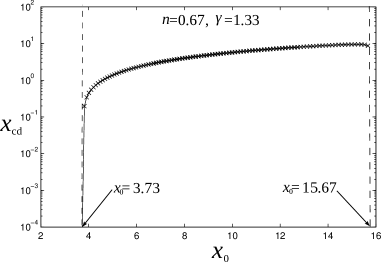
Figure 3: The relation of $x_{\text{cd}}$ (where $\alpha_{\text{cd}}$ and $v_{\text{cd}}$ can be determined) versus $x_{0}$ for the conventional polytropic case of $n=0.67$ and $\gamma=1.33$. The light solid curve marked along with crosses (“$\times$”) corresponds to a branch of type-1 solutions, which is the only possible solution branch for $x_{0}\;\lower 4.0pt\hbox{${\buildrel\displaystyle<\over{\sim}}$}\;50$. That is, there are no type-2 solutions to reach $x_{\text{cd}}$ for $x_{0}\;\lower 4.0pt\hbox{${\buildrel\displaystyle<\over{\sim}}$}\;50$.

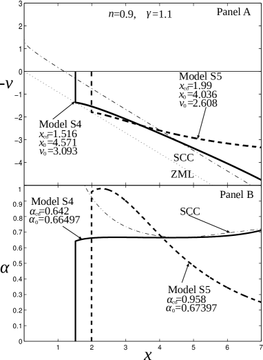
Figure 4: Conventional polytropic void solutions crossing the SCC smoothly with $n=0.9$ ($\gamma=1.1$). Panel A illustrates the profiles of negative reduced radial speed $-v(x)$ versus $x$ and Panel B shows the corresponding profiles of reduced mass density $\alpha(x)$ versus $x$. The dash-dotted curves in both panels are the SCC, while the light dotted line in Panel A represents the ZML. Two solutions of such type, marked by Model S4 and S5 (S for “smooth”) are plotted in heavy solid curve and heavy dashed curve, respectively. Model S4 is a type-2 solution crossing the SCC at $(x_{0},\ v_{0},\ \alpha_{0})=(4.571,\ 3.093,\ 0.66497)$ and Model S5 is a type-1 solution crossing the SCC at $(x_{0},\ v_{0},\ \alpha_{0})=(4.036,\ 2.608,\ 0.67397)$.

Among our self-similar solutions, it is possible for some to reach a specific line $nx=v$ which is referred to as the ZML. By eq. (8), the ZML leads to

$$m|_{nx=v}=\alpha x^{2}(nx-v)=0\ ,$$ (29)

and thus, according to eq. (5),

$$M|_{nx=v}=\dfrac{k^{3/2}t^{3n-2}}{(3n-2)G}m|_{nx=v}=0\ .$$ (30)

In other words, if there is a point in a solution where $v$ equals to $nx$, the enclosed mass $M$ within the corresponding radius of $nx=v$ (this radius expands with time $t$) would vanish.

On one hand, these would suggest that there is an expanding void, inside which mass and gravity could be neglected as compared with those of the surrounding gas shell, embedded inside a time-dependent and self-similarly evolving interface characterized by $nx=v$. On the other hand, condition $nx=v$ implies that the expanding interface represents a contact discontinuity (e.g. Lou & Zhai 2009, 2010) as revealed by the following relation

$$\dfrac{\mbox{d}r}{\mbox{d}t}=nk^{1/2}xt^{n-1}=k^{1/2}vt^{n-1}=u\ ,$$ (31)

at the time-dependent interface radius where $nx=v$. This is one of the necessary conditions for the existence of contact discontinuity (e.g. Lou & Hu, 2010) and the other requirement is the balance of pressures on both sides, which will be discussed in Section 4 presently. In the following, we invoke subscript “cd” to refer to those variables at the immediate outside of the contact discontinuity (for independent self-similar variable $x$ as an example, $x_{\text{cd}}$ is simply the similarity location of the contact discontinuity surface). For instance,

$$\alpha_{\text{cd}}=\lim_{x\rightarrow x_{\text{cd}}^{+}}\alpha(x)\ .$$ (32)

We note here several properties of solution adjacent to the void boundary from the gaseous envelope side. According to self-similar hydrodynamic ODE (6), we can determine the first derivatives at the ZML, viz.

$$\left.\dfrac{\mbox{d}v}{\mbox{d}x}\right|_{\text{cd}}=2(1-n)\ ,\qquad\quad\left.\dfrac{\mbox{d}\alpha}{\mbox{d}x}\right|_{\text{cd}}=\dfrac{n(1-n)}{(2-n)}\alpha_{\text{cd}}^{n}x_{\text{cd}}\ ,$$ (33)

and therefore the Taylor series expansions near the ZML are (this is actually the case of $q=0$ for a conventional polytropic gas in Hu & Lou, 2008; Lou & Hu, 2010)

$$\begin{split}v(x)&=nx_{\text{cd}}+2(1-n)(x-x_{\text{cd}})+\cdots\ ,\\ \alpha(x)&=\alpha_{\text{cd}}+\dfrac{n(1-n)}{(2-n)}\alpha_{\text{cd}}^{n}x_{\text{cd}}(x-x_{\text{cd}})+\cdots\ .\end{split}$$ (34)

Apparently, $\mbox{d}\alpha/\mbox{d}x$ at the contact discontinuity vanishes if $\alpha_{\text{cd}}=0$. This in turn hints that $\alpha(x)$ might be zero everywhere, and we have indeed verified this by extensive numerical explorations (see also Lou & Hu, 2010). Moreover, $\alpha_{\text{cd}}=0$ leads to a singularity for the second order derivative of $v(x)$ there (see Appendix A). In short, cases with $\alpha_{\text{cd}}=0$ are not physically acceptable for a conventional polytropic gas. Meanwhile for $m_{\text{cd}}=0$, we must have

$$\lim_{x\rightarrow x_{\text{cd}}^{-}}\alpha=0\ ,$$ (35)

indicating the presence of a jump or “cliff” in mass density across a contact discontinuity (this is exactly what the term “contact discontinuity” implies). The difference in mass densities inevitably leads to diffusion of gas particles across the contact discontinuity surface, which we shall discuss in Appendix D. We shall focus on void solution cases of non-vanishing $\alpha_{\text{cd}}>0$.

3.3 Conventional polytropic void solutions crossing the SCC smoothly

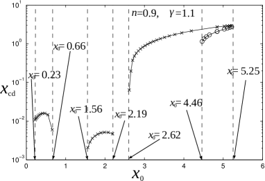
Figure 5: The relation of $x_{\text{cd}}$ (where $\alpha_{\text{cd}}$ and $v_{\text{cd}}$ can be determined) versus $x_{0}$ with $n=0.9$ ($\gamma=1.1$). The light solid curves marked along with crosses (“$\times$”) represent three branches of type-1 solutions, while those marked along with circles (“$\circ$”) represent one branch of type-2 solutions. Type-1 solutions are located in these intervals of $x_{0}$: $0.23<x_{0}<0.66$, $1.56<x_{0}<2.19$, $2.62<x_{0}<5.25$. Type-2 solutions, on the other hand, are located in one interval of $x_{0}$, i.e. $4.46<x_{0}<5.25$. The two rightmost branches of solutions in different type actually converge at $x_{0}\simeq 5.25$. In fact, it is the very point where the square root in eq. (17) vanishes and thus the two types of solutions are identical.

Conventional polytropic void solutions can cross the SCC smoothly without shocks. As shown in subsection 2.2, we are able to construct this kind of eigensolutions with central voids in self-similar evolution of dynamic expansion.

While usual schemes always involve plotting a $\alpha-v$ phase diagram by integrate towards a chosen meeting point, this series of void solutions can also be constructed as follows without resorting to the $\alpha-v$ phase diagram. First we choose a point $(x_{0},\ v_{0},\ \alpha_{0})$ as the sonic critical point on the SCC which satisfies ODEs (9) and (10). In fact, this represents a DOF. There, specific types (either type-1 or type-2, depending on which of the two $v^{\prime}$ we take) of $v^{\prime}$ and $\alpha^{\prime}$ are calculated consequently by solving eq. (15). After choosing a proper $\delta<0$, we calculate $v$ and $\alpha$ at $x=x_{0}+\delta<x_{0}$ and integrate inwards to see if it could reach the ZML; when this is fulfilled, let $\delta>0$ to obtain the reduced variables $v$ and $\alpha$ at $x=x_{0}+\delta>x_{0}$, we then integrate outwards to obtain a global solution for the self-similar dynamic evolution of an expanding central void.

In general, the SCC and ZML together enclose an area in the figure for presenting $v$ versus $x$ profiles. Obviously, it is necessary for a void solution to have part of itself inside this area since it should touch the ZML. Therefore, there is a necessary condition for a solution crossing the SCC smoothly to reach the ZML as

$$v^{\prime}<\dfrac{\mbox{d}v_{0}}{\mbox{d}x_{0}}\ ,$$ (36)

where $v^{\prime}$ carries the same meaning as in eq. (15), of a specific type (either type-1 or type-2). If this inequality is not satisfied along the whole SCC, we would expect no void solution that crosses the SCC smoothly of this type. It is straightforward to derive from eqs. (11) and (15) that the necessary condition for the existence of type-2 void solution (with smooth behaviour across the SCC) is $n>0.840$ at segment 1 of SCC (for the definition of “segment 1”, see eq. (11) as well as related discussions and definitions). By extensive numerical investigations, we find no type-2 solutions with $x_{0}$ less than $50$ for $n=0.67$, whereas for $n=0.9$, both types of void solutions exist.

As examples, we present several solutions ($n=0.67$ and $n=0.9$) crossing the SCC smoothly in Figs. 2 and 4, with the most important relevant parameter $x_{0}$ being chosen as $4.277$, $5.010$ and $6.084$ for Model S1, S2 and S3, respectively. All those with $n=0.67$ are type-1 void solutions, while there are both types of void solutions for $n=0.9$. Corresponding diagrams for the relation of $x_{\text{cd}}$ versus $x_{0}$ for $n=0.67$ and $n=0.9$ are displayed in Figs. 3 and 5, respectively.

3.4 Expanding void solutions with shocks

Figure 6: Presentation for the detachment (i.e. no cross-over) of the two phase curves in the phase diagram when $n$ decreases to $0.80$ (for the possible presence of shock solutions with EWCS envelopes). This detachment does not occur even when $n$ is only slightly greater than $0.80$ (say, $0.803$). To be specific, we compare $n=0.80$ cases with $n=0.815$ cases in this presentation. In all four panels, dashed curves marked with circles (“$\circ$”) are the phase curves representing different $x_{\text{s1}}$. The solid curve marked with crosses (“$\times$”) are the phase curves representing different $\alpha_{\text{cd}}$ and $x_{\text{cd}}\rightarrow 0^{+}$: these curves are the inner envelope of the “phase nets” with various combinations of $\alpha_{\text{cd}}$ and $x_{\text{cd}}$. Panels A1 and B1 illustrate the change of the phase curves in the “upper left region” (mainly for $x_{\text{s1}}<x_{\text{e}}$) while $n$ decreases from $0.815$ (Panel A1) to $0.80$ (Panel B1). Panels A2 and B2, meanwhile, present this change in the “lower right region” (for $x_{\text{s1}}>x_{\text{e}}$) in the phase diagram. The detachment of the two phase curves (hence the detachment of the circled phase curve from the inner envelope of the “phase net”) is apparent from this presentation.

Shocks are another way by which solutions can go across the sonic critical surface. There is an extra DOF for void solutions with shocks: the shock location in the self-similar expansion. We have applied two types of numerical schemes to construct void solutions with shocks. The following are the general outlines of these two procedures, perhaps with minor modifications in dealing with specific integrations.

One computation procedure is to integrate inwards. For solutions with vanishing $|v|$ and $\alpha$ at $x\rightarrow\infty$ under consideration, we can use asymptotic solution (7) to determine the initial value of integration at an $x$ that is large enough (say, $x=30$). We also choose a self-similar shock location in the upstream flow at $x_{s1}$. Then we integrate inwards numerically using the standard fourth-order Runge-Kutta scheme, apply shock jump conditions (21) in self-similar form at $x=x_{\text{s1}}$, and continue to integrate inwards from $x_{s2}$ and see if the solution would gradually approach and eventually touch the ZML. When such a solution touches the ZML, a global void solution with shock can then be readily constructed. Meanwhile, values of dimensionless variables at the contact discontinuity, $x_{\text{cd}}$ ($v_{\text{cd}}=nx_{\text{cd}}$) and $\alpha_{\text{cd}}$, are determined in a consistent manner.

The other computation procedure is to integrate outwards. Choose the self-similar location of void boundary $x_{\text{cd}}$ and reduced mass density $\alpha_{\text{cd}}$ there, and decide the location $x_{\text{s2}}$ of shock on the downstream side. Then integration is taken outwards to a relatively large value of $x$ with respect of the jump at the shock by applying shock conditions (21) (note the commutation symmetry with regard to subscripts 1 and 2 discussed in subsection 2.3). The mass and speed parameters $A$ and $B$ to characterize the asymptotic solution behaviours at large $x$ can also be evaluated with the value of $v(x)$ and $\alpha(x)$ at a very large $x$ by using eq. (7).

Practically, there is not much difference between the two kinds of void solution construction procedures except when parameters chosen in highly “sensitive” regimes. We have applied both numerical integration procedures as cross-checks of each other for the reliability of our void solutions.

3.4.1 Expanding void solutions with EWCS envelope

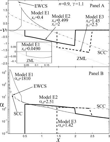
Figure 7: Void solutions with shocks and EWCS envelopes; Panel A for the negative reduced radial velocity $-v(x)$ versus $x$ profiles and Panel B for the reduced mass density $\alpha(x)$ versus $x$ profiles. These conventional polytropic solutions have $n=0.9$ ($\gamma=1.1$). The SCCs in both panels are presented by dash-dotted curves, while the ZML in Panel A is shown by dotted line. Models E1 (“E” for “EWCS”), E2 and E3 are shown by light solid curve, heavy solid curve and heavy dashed curve, respectively. The envelopes beyond the shock of Models E2 and E3 are the same: SPS (thus $x_{\text{s1}}>x_{\text{e}}$) solution, but the locations of the shocks are different. Model E1, on the other hand, has $x_{\text{s1}}<x_{\text{e}}$.

The outer part of EWCS is identical to the static SPS solution, namely (e.g. Suto & Silk, 1988, with $n+\gamma=2$)

$$v=0\ ,\qquad\qquad\alpha=\left[\dfrac{2(2-n)(3n-2)}{n^{2}}\right]^{1/n}x^{-2/n}\ ,$$ (37)

beyond the expansion wave radius ($x_{\text{e}}$ for the similarity location of this radius), i.e. $x>x_{\text{e}}$. For $n=1$, this type of polytropic solution becomes the outer part of a singular isothermal sphere (SIS; e.g. Lou & Zhai, 2009, 2010). The asymptotic behaviour of this kind of EWCS at small $x$ is given by (e.g. Suto & Silk, 1988; Lou & Wang, 2006)

$$v=-\left[\dfrac{2m(0)}{(3n-2)x}\right]^{1/2}\ ,\qquad\alpha=\left[\dfrac{(3n-2)m(0)}{2x^{3}}\right]^{1/2}\ ,$$ (38)

where constant $m(0)$ represents the central mass point.

We have obtained shock solutions with central void and EWCS envelope. When a specific envelope is prescribed, there is only one DOF, viz., the shock location. The technique of $v$ versus $\alpha$ “phase net”, a variation of $v$ versus $\alpha$ phase diagram scheme [Hunter (1977) and the “phase net” was developed in Lou & Zhai (2009, 2010)], is applicable because of the similar situation. Steps of the scheme are summarized below. We first obtain the EWCS envelope by numerical integration. Choose a meeting point $x_{\text{F}}$ and the similarity upstream location of the shock $x_{\text{s1}}$. With shock jump conditions applied for connecting $x_{\text{s1}}$ and $x_{\text{s2}}$, we numerically integrate from $x_{\text{s2}}$ to $x_{\text{F}}$ and record the value of $v$ and $\alpha$ there. Select a series of $x_{\text{s1}}$ values, get a series of $(v,\ \alpha)$ pairs at $x_{\text{F}}$ and use these $(v,\ \alpha)$ pairs to plot a curve, on which different points correspond to different values of $x_{\text{s1}}$, in the phase diagram. Then we select a series of $x_{\text{cd}}$ and $\alpha_{\text{cd}}$ in pairs and do similar things: integrate towards $x_{\text{F}}$ and get a sequence of curves or a “net” [i.e., the so-called “phase net” in Lou & Zhai (2009)] in the phase diagram corresponding to different $x_{\text{cd}}$ and $\alpha_{\text{cd}}$ in pairs.

Applying this scheme, we have explored various void solutions with static polytropic envelopes. We find numerically that when the scaling index $n$ is less than $0.80$, there appears to be no such type of solutions with one shock. We realize for any specific $n$ that the curve representing $x_{\text{s1}}$ is actually bounded in the phase diagram and “shrinks” as $n$ increases. Meanwhile, the “net” with different $x_{\text{cd}}$ and $\alpha_{\text{cd}}$ pairs has an inner envelope (actually this envelope is outlined by the curve with different $\alpha_{\text{cd}}$ and $x_{\text{cd}}\rightarrow 0^{+}$). When $n$ becomes greater than $0.80$, there are two regions in the diagram where the $x_{\text{s1}}$-curve intersects the “net”: one corresponds to the solutions with $x_{\text{s1}}<x_{\text{e}}$, and the other, $x_{\text{s1}}>x_{\text{e}}$ (in the phase diagram, these two regions are clearly separated). However, when $n$ becomes less than $0.80$, the $x_{\text{s1}}$-curve detaches from the net and neither of the two intersecting areas can still exist. We have tried various values of $x_{\text{F}}$ from $0.01$ to $20$ and only find the same threshold of $n=0.80$.

We shall refer to the region with $x_{\text{s1}}<x_{\text{e}}$ as the “upper region” and that with $x_{\text{s1}}>x_{\text{e}}$ as the “lower region” in the caption of Fig. 6 because in a more complete phase diagram, the “upper region” always appears on the upper-left corner while the “lower region” is always on the lower-right corner. These terminologies can be readily clarified by referring to figure 7 of Lou & Zhai (2009) for an isothermal case. In addition, if there is no EWCS-envelope void solution (with shock), there will be no breeze solution with a void and a shock either. We have found that if $0<A<A_{\text{e}}$ and $B=0$ (hence $v>0$ at large $x$), the curve for $x_{\text{s1}}$ will “shrink” even more, further preventing $x_{\text{s1}}$ curve from intersecting the “net”. Furthermore, the decrease of $B$ parameter also leads to a “shrink” of $x_{\text{s1}}$ curve, therefore contraction and inflow solutions become much more difficult to exist.

This detachment in the phase diagram related to the scaling index $n=0.8$ is illustrated by examples in Fig. 6. Note that this separation by $n\;\lower 4.0pt\hbox{${\buildrel\displaystyle<\over{\sim}}$}\;0.8$ is valid for conventional polytropic cases only; there is no such separation for general polytropic cases as shown in Hu & Lou (2008). Note also that void solutions with EWCS envelope and shock may still exist if the solutions cross the sonic critical surface for more than once (crossing smoothly or by shock discontinuity).

Several void solution examples of this type are presented in Fig. 7 with $n=0.9$ (thus $\gamma=1.1$) and $x_{\text{s1}}$ being $0.4$, $2$, and $2.5$, respectively.

3.4.2 Void solutions with various dynamic envelopes: breeze, contraction, outflow and inflow

With relevant parameters summarized in Table 1, a series of self-similar void solutions are obtained with shocks and $n=0.67$ (values of $n$ are to be discussed in subsection 4.2).

Models 1 through 4 are four kinds of void solutions: those that have breeze, contraction, outflow and inflow envelopes, respectively, all with $n=0.90>0.80$. Their solutions are illustrated in Fig. 8 to show in non-dimensional form the profiles of reduced radial velocity $v(x)$ and reduced mass density $\alpha(x)$ (definitions of these four kinds of envelopes are given in subsection 2.1). Models 5 through 7 are void solutions with outflow envelope beyond the shock with $n=0.67<0.80$, which we shall elaborate for further applications. These solutions are displayed in Fig. 9.

In numerical explorations for cases of $n=0.67$, we have found that even for strong outflows, there are impressive trends to fall inwards at some intervals of $x$: this is clearly the results of self-gravity. This point is unambiguously illustrated by Models 5 through 7, and other models not shown here also appear similarly in this aspect. We shall further discuss this feature in subsection 4.4.

Table 1: Parameters specifying conventional polytropic void solutions with shocks. The first four models all have $n=0.9$ while the last three all have $n=0.67$. These solutions are constructed by integrating inwards and we confirmed their correctness by integrating outwards within the tolerance of numerical errors.

Model	$n$	$A$	$B$	$x_{\text{s1}}$	$\eta_{k}$	$x_{\text{cd}}$	$\alpha_{\text{cd}}$
1	0.9	3	$-1$	1.5	0.826	0.809	13.9
2	0.9	3	1	3.5	0.902	2.509	1.01
3	0.9	2.542	0	2.5	0.905	1.559	2.03
4	0.9	1.542	0	2.5	0.950	1.204	0.88
5	0.67	2.43	13.6	5.5	0.214	0.239	59.6
6	0.67	2.25	13.2	7	0.300	1.031	12.6
7	0.67	4.50	16.7	9	0.145	0.358	28.2

Figure 8: Presentation of negative reduced radial flow velocity $-v(x)$ versus $x$ (Panel A) and reduced mass density $\alpha(x)$ versus $x$ (Panel B) for shock void solutions with inflow (heavy solid curve), outflow (heavy dashed curve), contraction (light dashed curve) and breeze (light solid curve) envelopes specified by Models 1 through 4 in Table 1, respectively. The SCCs in both Panels A and B are shown by dash-dotted curves; the ZML is represented by the light dotted curve.

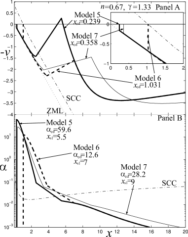
Figure 9: Presentation of negative reduced radial flow velocity $-v(x)$ versus $x$ (Panel A) and reduced mass density $\alpha(x)$ versus $x$ (Panel B) for outflow-envelope solutions specified by Models $5-7$ in Table 1. The dash-dotted curves in both panels are the SCCs. The light dotted line in Panel A is the ZML. Among the three solutions, Models 5, 6 and 7 are illustrated with heavy solid curve, heavy dashed curve and light solid curve, respectively. The small inset at the upper-right corner of Panel A is a zoom of solution curves near the origin $x=0$ and $-v=0$.

4 Astrophysical Applications

There are several astrophysical situations where hot tenuous bubbles exist, shaped up by pertinent physical mechanisms. Here, we discuss cases that might be capable of describing the evolution of supernova at an early stage (the so-called “optically thick” stage), during which the predominant driving power inside the stellar envelope could possibly be the pressure of some extremely relativistic particles such as neutrinos and photons trapped inside a central cavity. Some necessary aspects need to be addressed before outlining our model scenario.

4.1 Formation of a central bubble or cavity

Research works have hinted at a scenario that a cavity can be formed surrounding the centre of a supernova during the initial phase. As concluded by Bethe (1990), accelerating infall of substances is inhibited by powerful neutrino pressure from the neutrinosphere before neutrinos decouple from the gas and escape; moreover, a rebound shock may be revived when the intense neutrino flux is absorbed by surrounding nuclear matters at a radius $r\sim 100\mbox{ km}$ or more. Such a mechanism can drive materials around the core outwards and shape up a rarified bubble or cavity, which is clearly illustrated in figure 2 of Bethe & Wilson (1985). This perspective was further strengthened by simulations of Janka & Hillebrandt (1989a, b) and Janka & Müller (1996), revealing the formation of a bubble around the centre of a supernova, filled with intense electromagnetic radiation field and other relativistic materials.

4.2 Pressure balance, EOS, and the central power

While it is allowed to be discontinuous in mass densities and temperatures across the contact discontinuity surface, a pressure balance across this contact surface should be maintained to fulfill the necessary mechanical requirement. Here, we discuss consequences for the conventional polytropic EoS and some relevant aspects of the required pressure balance.

For an extremely relativistic degenerate or hot gas, statistical mechanics gives an adiabatic EoS (e.g. Callen, 1985),

$$p\rho^{-4/3}=\mbox{constant}\ .$$ (39)

With a spherical volume $V=4\pi r^{3}/3$, $\rho$ is the mass density, $p$ is the pressure, and the energy density is simply gotten by a multiplication of $c^{2}$ with $c$ being the speed of light.

Consider matters inside a highly rarified central cavity. For a temperature as high as $\sim 1-10\mbox{ MeV}/k_{\text{B}}$ or more, it is natural to expect substances (i.e. radiation field and products of electron-positron pair production processes) inside the cavity to be relativistic. During the self-similar dynamic expansion of a central void, transformation (5) gives $r_{\text{cd}}\propto t^{n}$. Assuming that the mass (hence energy) inside the void is to be homogeneous and conserved (adiabatic) during the self-similar expansion, thermal pressure $p$ is thus proportional to $V^{-4/3}\propto r_{\text{cd}}^{-4}$ (for relativistic matters, the speed is almost the speed of light $c$; hence homogeneity would be a sensible approximation for a not very large scale, say $\;\lower 4.0pt\hbox{${\buildrel\displaystyle<\over{\sim}}$}\;c\times 1\mbox{ s}$). From those, we conclude that $p\propto t^{-4n}$ for relativistic matters inside a void at the boundary (i.e., the surface of contact discontinuity).

On the other hand in terms of the surrounding gas envelope in self-similar evolution, the thermal pressure just outside the contact surface is proportional to $t^{2n-4}$ by transformation (5); a contact surface has constant $\alpha_{\text{cd}}$ and $x_{\text{cd}}$ in a self-similar dynamic evolution. There should be a sustained pressure balance across the contact surface, requiring at least the same time-dependence of pressures on both sides of a contact discontinuity. With this consideration alone, we would require $n=2/3$ from $2n-4=4n$ (i.e. $\gamma=4/3$ from $n+\gamma=2$).

We shall not consider the exact case of $n=2/3$ for a homologous flow as done by Goldreich & Weber (1980), Yahil (1983), and Lou & Cao (2008). Instead, we invoke a physically more plausible condition $n=2/3+\epsilon$ with $\epsilon\;\lower 4.0pt\hbox{${\buildrel\displaystyle>\over{\sim}}$}\;0$ being a real number slightly greater than zero (e.g., $n=0.67$) to describe a small deviation from an adiabatic process for extremely relativistic matters inside a cavity, with a tacit assumption that the central compact remnant (e.g. a nascent neutron star or a nascent stellar mass black hole) continues to input energy into the “void” with a time-dependent rate, usually a decreasing one.

Simple thermodynamic and mechanical considerations yield that an $\epsilon$ added to $n$ reflects some physical mechanisms adding more energy into a void during its dynamic expansion, viz.

$$\mbox{d}Q\simeq 3\epsilon p\mbox{d}V\ ,$$ (40)

where $Q$ is the amount of heat input into a void by some mechanisms as shown in Appendix B.

By transformation (5), we readily derive

$$\dfrac{\mbox{d}Q}{\mbox{d}t}=3\epsilon\left(\dfrac{2}{3}+\epsilon\right)\alpha_{\text{cd}}^{4/3-\epsilon}x_{\text{cd}}^{3}\dfrac{k^{5/2}t^{5\epsilon-5/3}}{G}\ ,$$ (41)

where $G$ is the gravitational constant and $k$ is the same sound parameter in transformation (5), and the subscript “cd” denotes quantities related to the contact discontinuity. The sound parameter $k$ should be evaluated with in terms of dimensional values such as $\rho_{\text{cd}}$, which depends on specific applications of our void model.

We do not yet know the specific form(s) of energy release from the central compact object into the surrounding cavity. We consider simple cases as examples of model consideration.

There is a sensible physical possibility that the energy input comes mainly from the thermal radiation from the collapsing central compact object. As is conventional in study of neutron star cooling process, an “effective” temperature $T_{\text{e}}$ is often introduced to indicate the ability of photon radiation (e.g. Yakovlev & Pethick, 2004; Page et al., 2006). Note that even though neutrino cooling is much more important than photon cooling during this epoch, photon radiation is much more important for a sustained expansion of central void (see subsection 4.3 for details). With this $T_{\text{e}}$ specified, the radiation energy flux input into the bubble is given by

$$\dfrac{\mbox{d}Q}{\mbox{d}t}=4\pi r_{\text{n}}^{2}\sigma T_{\text{e}}^{4}\ ,$$ (42)

where $r_{\text{n}}$ is the radius of the proto-neutron star and $\sigma=5.6705\times 10^{-5}\mbox{ erg cm}^{-2}\mbox{ s}^{-1}\mbox{ K}^{-4}$ is the Stefan-Boltzmann constant. Combining eqs. (41) and (42) with $n=2/3+\epsilon$, we obtain a scaling of $T_{\text{e}}$ as a function of $t$ in the form of

$$T_{\text{e}}\propto t^{5(n-1)/4}\ .$$ (43)

If simplified calculations of Page et al. (2006) hold even in the early evolution phase of a proto-neutron star, we obtain approximately for a “slow” (“standard”) cooling process, $T_{\text{e}}\propto t^{-1/12}$ and thus $n=14/15\simeq 0.933$, while for a “fast” cooling process, $T_{\text{e}}\propto t^{-1/8}$ and thus $n=0.9$.

As an example, let us approximately calculate the amount of energy input rate with respect to the model applied in our scenario for SN1993J in subsection 4.5.2. The dimensionless model applied there has $x_{\text{cd}}=2$ and $\alpha_{\text{cd}}=10^{-3}$ with $n=0.933$ (in addition, the relevant $x_{\text{s2}}$ is $3.3$). The dimensional counterpart is taken as what is specified in Fig. 11 at $t=11\mbox{ s}$. We then have the sound parameter $k=1.584\times 10^{18}\mbox{ c.g.s. unit }$ and thus from eq. (41)

$$\dfrac{\mbox{d}Q}{\mbox{d}t}\simeq 8\times 10^{49}\mbox{ erg s}^{-1}\ .$$ (44)

A thermal luminosity as high as this would be possible in a very early stage in terms of pertinent calculations of Page et al. (2006) in their figure 14. For $r_{\text{n}}=10\mbox{ km}$, we obtain from eq. (42) an effective temperature $T_{\text{e}}\simeq 1.8\times 10^{10}\mbox{ K}$ at that time, corresponding to a very early epoch of a proto-neutron star (see again figure 14 in Page et al. 2006 for a high surface temperature of a strange star). This temperature $T_{\text{e}}$ is much higher than the radiation temperature in the bubble (see Fig. 11). Moreover, the temperature in the bubble drops at a rate proportional to $t^{n/2-1}=t^{-0.534}$, which is much faster than $T_{\text{e}}\propto t^{-1/12}$. This can be seen from the pressure confining the central bubble $p=p_{\text{cd}}\propto t^{2n-4}$ [see also transformation (5)] and $p\propto T^{4}$ for radiation [see eq. (3.53) in Callen (1985)].

To continue the above consideration, we may presume approximately a black body emission spectrum from an isothermal proto-neutron star. If the heat capacity at constant volume of a proto-neutron star depends on the temperature in a power-law form, viz. $C_{V}\propto T^{\xi}$ with $\xi$ being an exponent, we have

$$T_{\text{n}}^{\xi}\mbox{d}T_{\text{n}}\propto\mbox{d}U_{\text{n}}\propto-T_{\text{n}}^{4}\mbox{d}t\ ,$$ (45)

where $U_{\text{n}}$ is the internal energy of the proto-neutron star. From that, we immediately derive the proportional relation $T_{\text{n}}\propto t^{1/(\xi-3)}$ or

$$\dfrac{\mbox{d}Q}{\mbox{d}t}=-\dfrac{\mbox{d}U_{\text{n}}}{\mbox{d}t}\propto T_{\text{n}}^{4}\propto t^{4/(\xi-3)}\ .$$ (46)

In reference to eq. (41), we need to require $4/(\xi-3)=5\epsilon-5/3$, leading to the following relation between $n$ and $\xi$

$$n=1+4/[5(\xi-3)]\ .$$ (47)

Since for a degenerate Fermi gas, theoretical computations of heat capacity at constant volume $C_{V}$ gives the exponent $\xi$ range of $0<\xi<1$ (e.g. Greiner et al., 1995, from its figure 14.2). It follows that scaling index $n$ would be restricted to the range $3/5<n<11/15$ according to eq. (47). Actually, we should require $n>2/3$ in our formulation for physical similarity solutions. In other words, the mechanism attributing the energy input to the black body radiation from a central proto-neutron star to a surrounding hot bubble or cavity can only be responsible for the cases where inequality $2/3<n<11/15$ is satisfied. We emphasize that if for some reason, $\xi$ is allowed to be negative, then the value of $n$ may approach 1. For other physical mechanisms of energy input into the central cavity from a proto-neutron star, inequality $n<11/15$ may not be necessary. For example, numerical simulations of Thompson et al. (2001) have offered a neutrino luminosity proportional to $t^{-0.9}$ (see their figure 9) after a SN explosion and this would correspond to $n=0.82>11/15$.

4.3 Momentum transfer by scattering processes

The initial rapid detachment of an out-flowing envelope from a collapsing compact core is primarily accomplished by a powerful neutrino pressure (e.g. Bethe, 1990). After hundreds of milliseconds, energetic neutrinos decouple from surrounding gas materials and escape, an important source of driving power for the bubble expansion vanishes.

Even though the radiation (mainly involving trapped photons and electron-positron pairs produced by pair production) is relatively weaker in luminosity than neutrinos, scattering process, by which the momentum and energy are transferred, of photons by matters in the gas shell is nevertheless much more effective.

Meanwhile, previous studies have implied that the amount of energy needed to blow a massive stellar envelope up is roughly at the same magnitude ($\sim 10^{51}\mbox{ erg}$) as that radiated by photons in SN explosion (see Janka & Müller 1996 for details; this estimate could also be derived from an integration of the energy spectrum in Chevalier 1974). These also suggest that trapped photon radiation may be a major driving power of further detachment between a collapsing core and an expanding massive envelope after neutrinos have already shaped an initial central cavity and decoupled from surrounding gas materials.

Such a model consideration is outlined in the following subsection, where we compare the contributions of neutrino flux and of photon radiation field. We will examine the possibility of photon radiation field of being an important driving power to the expansion of a shocked massive envelope and a sustained central void expansion.

4.3.1 Scattering of neutrinos by heavy nuclei

Energetic neutrinos are important in the initiation and evolution of SN explosions (e.g. Bethe, 1990). Scattering process of neutrinos with extremely high density matters is treated as coherent scattering, with a scattering cross section $\Sigma_{\nu}$ given by (e.g. Tubbs & Schramm, 1975)

$$\Sigma_{\nu}\sim 10^{-45}\mbox{ cm}^{2}A^{2}\left(\dfrac{E_{\nu}}{m_{\text{e}}c^{2}}\right)^{2},$$ (48)

where $A$ is the number of nucleons in one nucleus, $E_{\nu}$ is the neutrino energy, $m_{\text{e}}$ is the electron mass and $c$ is the speed of light. The electron rest mass energy $m_{\text{e}}c^{2}$ comes basically from the process $\text{n}\rightarrow\text{p}+\text{e}^{-}+\bar{\nu}_{\text{e}}$ in a nuclear reaction. Equation (48) does not include $\mu$ neutrinos $\nu_{\mu}$ ($\bar{\nu}_{\mu}$) and $\tau$ neutrinos $\nu_{\tau}$ ($\bar{\nu}_{\tau}$), because the latter two are much less significant as compared with electron neutrinos $\nu_{\text{e}}$ ($\bar{\nu}_{\text{e}}$).

For a highly degenerate dense stellar core, the scattering of neutrinos are so effective that a central “neutrino bubble” on a spatial scale of $\sim 100\mbox{ km}$ is shaped up by the extremely intense neutrino flux released from the collapsed core (e.g. Bethe, 1990; Padmanabhan, 2001). In this case, the mean free path of electron neutrinos $\lambda_{\nu}$ is given by (e.g. Padmanabhan, 2001)

$$\lambda_{\nu}\simeq 3\times 10^{4}\mbox{ cm}\left(\dfrac{\bar{A}}{56}\right)^{-2}\left(\dfrac{\rho}{10^{12}\mbox{ g cm}^{-3}}\right)^{-5/3}\ ,$$ (49)

where $\bar{A}$ is the average number of nucleons per nucleus. On the other hand, the shaping of the neutrino bubble causes the matters surrounding the core to expand significantly, making them less dense and non-degenerate gradually (see Appendix D). For a non-degenerate gas envelope, $\lambda_{\nu}$ is estimated by

$$\lambda_{\nu}\simeq\dfrac{\bar{A}m_{\text{p}}}{\Sigma_{\nu}\rho}\sim 0.5R_{\odot}\bar{A}^{-1}\left(\dfrac{E_{\nu}}{1\mbox{ MeV}}\right)^{-2}\left(\dfrac{\rho}{10^{10}\mbox{ g cm}^{-3}}\right)^{-1}.$$ (50)

This $\lambda_{\nu}$ would be too long to accomplish an effective momentum transfer for a mass density less than that of nuclear matters. Therefore we expect the material shell to be transparent for neutrinos shortly after a “neutrino bubble” being shaped up.

4.3.2 Scattering of photons by charged particles

Classical and semi-classical theories yield almost the same result for the scattering cross section $\Sigma_{\text{ph}}$ between a photon and a charged particle, usually referred to as the “Thomson cross section” given by (e.g. Jackson, 1999)

$$\Sigma_{\text{ph}}=\dfrac{8\pi}{3}\left(\dfrac{e^{2}}{mc^{2}}\right)^{2}\ ,$$ (51)

where $e=4.803\times 10^{-10}\mbox{ e.s.u.}$ is the electron charge, $m$ is the charged particle mass and $c$ is the speed of light.

Clearly, Thomson cross section is much larger for electrons than for nuclei because $m_{\text{e}}\ll m_{\text{p}}$ (specifically for electrons, $\Sigma_{\text{ph}}=6.65\times 10^{-25}\mbox{ cm}^{2}$). For a fully ionized plasma of mass density $\rho$, we obtain the mean free path of photons ($n_{\text{nuc}}$ and $n_{\text{e}}$ are the number densities of nuclei and electrons, respectively):

$$\lambda_{\text{ph}}=\dfrac{1}{n_{\text{nuc}}\Sigma_{\text{ph,nuc}}+n_{\text{e}}\Sigma_{\text{ph,e}}}\simeq\dfrac{1}{\Sigma_{\text{ph,e}}n_{\text{e}}}\ .$$ (52)

Numerically, we estimate a photon mean free path as

$$\lambda_{\text{ph}}\simeq 5\mbox{ cm}\left(\dfrac{\rho}{1\mbox{ g cm}^{-3}}\right)^{-1}\ .$$ (53)

This implies that photons are tightly trapped inside the cavity even for an envelope mass density as low as $\sim 10^{-5}\mbox{ g cm}^{-3}$. The much higher efficiency of momentum transfer (compared with neutrinos) also permits the possibility of radiation-driven envelope expansion of a void.

4.4 Void solutions as asymptotic conditions

Figure 10: Dimensional model presentation at $t=t_{i}$ (the initial timescale of a self-similar void evolution). Panels A, B and C illustrate the radial flow velocity (in unit of $10^{9}\mbox{ cm s}^{-1}$), mass density (in unit of $\mbox{g cm}^{-3}$) and temperature (in unit of Kelvin K) profiles of the model, respectively. Vertical line-sections in the plot on the left represents the contact surface, inside of which is the intense radiation field, while those on the right indicates the expanding shock. Note that we have also shown the temperature of the radiation field inside the central cavity in Panel C.

The mass is conserved in evolution and thus mass densities throughout the envelope decrease as time goes on for an overall expansion. Since we investigate the situation that radiation field continues to drive the envelope outwards, when the gas in the inner envelope (especially near the contact discontinuity surface) becomes sufficiently tenuous, trapped photons can leak out gradually.

We define $\Delta t$ as the time duration after $t_{i}$ (for its definition see Appendix C; hereafter we use subscript “i” for those initial values in dynamic void evolution) to the time that the mass density near the contact discontinuity becomes fairly low (e.g. $\rho_{\text{cd}}\sim 10^{-5}\mbox{ g cm}^{-3}$, see subsection 4.3.2).

In reference to similarity transformation (5), an estimate of $\Delta t$ is given by

$$\Delta t\sim t_{i}\left[\left(\dfrac{\rho_{\text{cd},i}}{10^{-5}\mbox{ g cm}^{-3}}\right)^{1/2}-1\right]\ .$$ (54)

Meanwhile, the diffusion across the contact discontinuity may modify our model. In fact, diffusion process is not so effective as analyzed in Appendix D.

The mass density near the contact discontinuity is attenuated in a self-similar expansion, which would make our radiation driving expansion model invalid after a sufficiently long lapse in time. We here show that our self-similar model may be further used as an asymptotic solution when the radiation-driving mechanism is no longer effective.

Recalling self-similar transformation (5), the pressure decreases with $p_{\text{cd}}\propto t^{2n-4}$, while the radius of the contact discontinuity expands with a power law $t^{n}$. We define the integral of radiation pressure $p_{\text{cd}}$ over the contact discontinuity surface as the “radial radiation force” $F_{r}$,

$$F_{r}=4\pi r_{\text{cd}}^{2}p_{\text{cd}}=x_{\text{cd}}^{2}\alpha_{\text{cd}}^{\gamma}\dfrac{k^{2}t^{4n-4}}{G}\ .$$ (55)

This result indicates that the force exerted on the gas shell by the radiation inside the bubble becomes less and less important as time goes on, since there is usually $4(n-1)<0$ (from $\gamma>1$ and $n+\gamma=2$). For a long enough time $t$, the pressure force across the contact discontinuity surface diminishes to a negligible level. In other words, even though there should be a certain pressure across the contact discontinuity surface, the dynamics of the shell are not significantly influenced if those pressures are weakened when $t$ becomes sufficiently large. This analysis enables us to regard our void model to be valid as an asymptotic solution in the epoch when the gas shell becomes “optically thin” and thus radiation in the bubble leaks out.

As an example, for the model parameters specified in Table 2, if we take $\rho_{\text{cd}}\sim 10^{-5}\mbox{ g cm}^{-3}$ as the transition criterion from “optically thick” to “optically thin”, we get

$$p_{\text{cd}}|_{\rho_{\text{cd}}=10^{-5}\text{ g }\text{cm}^{-3}}=3\times 10^{6}\mbox{ dyn cm}^{-2}\ .$$ (56)

This is a low pressure in comparison with the inertia of the stellar envelope. We evaluate the “radial radiation force” exerted by the radiation pressure as

$$F_{r}=4\pi r_{\text{cd}}^{2}p_{\text{cd}}\sim 10^{33}\mbox{ dyn}\ .$$ (57)

As a result, even though central radiation field has gone and there may be many deviations from the original formation (e.g., the shock may eventually die out, asymmetry may become more apparent, diffusion across the contact surface may become severe), void solutions are still reasonable to the degree of (at least) approximations, since the inertia becomes predominant in further continuation of expansion.

4.5 Self-similar evolution of SNe driven by
   central photon radiation pressure

In this subsection, we briefly discuss a few specific applications of the conventional polytropic self-similar void solutions with shocks in the context of SNe. The procedure of constructing a physical model from dimensionless solutions are summarized in Appendix C.

4.5.1 A dynamic void model of self-similar evolution

Table 2: Parameters specifying conventional polytropic void models with shocks; in dimensional form, they describe the dynamic evolution of a gas shell, e.g. a SN. “CD” in this Table denotes the contact discontinuity. “Duration time” is the time span of the model validity considering the scattering process of the charged particles by photons (see subsection 4.4 for details).

Item	Variable Name	Value
Total mass	$M$	$\sim 20M_{\odot}$
Density at CD	$\rho_{\text{cd},i}$	$\sim 4.7\times 10^{10}\mbox{ g }\mbox{cm}^{-3}$
Pressure at CD	$p_{\text{cd},i}$	$\sim 10^{29}\mbox{ dyn }\mbox{cm}^{-2}$
Initial void radius	$r_{\text{cd},i}$	$\sim 160\mbox{ km}$
Radial velocity of CD	$u_{\text{cd},i}$	$\sim 6000\mbox{ km s}^{-1}$
Cavity Temperature	$T_{\text{rad},i}$	$\sim 9\times 10^{10}\mbox{ K}$
Duration time	$\Delta t$	$\;\lower 4.0pt\hbox{${\buildrel\displaystyle>\over{\sim}}$}\;10^{6}\mbox{ s}$

By properly specifying similarity transformation and envelope cutoff (see Appendix C), we would adopt our Model 6 with key parameters summarized in Table 1 to describe a self-similar void evolution for a model SN. The progenitor has a mass of $\sim 20M_{\odot}$. An envelope cutoff radius is set at $r_{\text{cut}}\simeq 40R_{\odot}$ where the mass density is $\rho_{\text{cut}}\simeq 10^{-8}\mbox{ g cm}^{-3}$ and the gas temperature is taken as $T\simeq 4000\mbox{ K}$.

Before the phase of self-similar evolution, a cavity around the center has already been carved out by the powerful neutrinosphere, before neutrinos decouple from the surrounding envelope and escape. The cavity radius is initially estimated as $\;\lower 4.0pt\hbox{${\buildrel\displaystyle>\over{\sim}}$}\;100\mbox{ km}$, by Bethe & Wilson (1985), Bethe (1990) and later works on the Wilson mechanism such as Janka & Müller (1996). Here we take the initial cavity radius $r_{\text{cd},i}$ to be $\sim 160\mbox{ km}$. Subsequently, the stellar envelope surrounding the cavity expands outwards continuously powered by photon radiation pressure during the following self-similar evolution. Some important numerical values of parameters for describing this model (which also specifies the similarity transformation) are given in Table 2.

While $\Delta t$ (defined in subsection 4.4) is presented in Table 2, we note that the model can remain valid after this $\Delta t$ as a asymptotic condition noted in subsection 4.4.

As an example, radial flow velocity, density and temperature profiles at the initial stage ($t=t_{i}$) are displayed in Fig. 10. From Panel A of Fig. 10, we observe the impact of the radiation-driven mechanism in the dynamic evolution of envelope with an expanding central void. While the radial flow speed throughout the shell remains always positive and large, there are still intervals of radius where gas materials show an impressive trend to collapse inwards under self-gravity. In fact, a quick glance at some other self-similar models with $\gamma$ in EoS being close to $4/3$ suggests a strong trend of the shell to decelerate (or even collapse) in the upstream side of a shock (see Models 5 and 6). The expanding shock here serves as an important and effective accelerator to drive the envelope outwards against self-gravity.

Regarding our analysis of self-similar model, the photon radiation field trapped inside the central bubble appears to be a physically plausible candidate of the energy source, which drives the envelope outwards continuously during the optically thick phase. From Panels B and C of Fig. 10, we readily recognize an outgoing shock. It is a strong shock with a drastic jump across the shock front in both mass density and temperature. The contact discontinuity surface at $r_{\text{cd},i}=160\mbox{ km}$ initially, on the other hand, was supported by the strong neutrino flux before the decoupling of neutrinos. The neutrino flux also heats up rarified materials inside the void significantly and is responsible for the discontinuity in temperature across the contact interface.

4.5.2 Supernova SN1993J

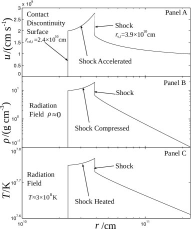
Figure 11: Possible fittings of radial velocity ($u$ in Panel A), mass density ($\rho$ in a logarithmic scale in Panel B) and temperature ($T$ in a logarithmic scale in Panel C) versus radius ($r$ in a logarithmic scale) profiles of SN1993J ejecta in the early stage (a timescale of $\sim 10\mbox{ s}$). The “shell” region between the contact discontinuity and the shock is $\sim 30\%$ of the shock radius, in accordance with radio observations (e.g. Marcaide et al., 2009).

SN1993J in M81 is a type-IIL core collapse supernova about $3\mbox{ Mpc}$ away from us (e.g. Schmidt et al., 1993). This close neighborhood has enabled a plethora of observations. Here we take the observation and simulation results presented in Martí-Vidal et al. (2011a, b) and references therein. SN1993J has a spherical asymmetry $\;\lower 4.0pt\hbox{${\buildrel\displaystyle<\over{\sim}}$}\;2\%$ and it would be of considerable interest to explore the capability of our void model with spherical symmetry. Numerical simulations of Martí-Vidal et al. (2011a, b) have adopted the dynamic model of Chevalier (1982) where the self-gravity is neglected.

There are different fittings of SN1993J expansion presented in Martí-Vidal et al. (2011a) with various expansion parameter $m$ (not the reduced mass here) which takes the similar connotation as $n$ in our formulation. An accepted selection of $n$ seems to be $n=0.933$ before $\sim 360\mbox{ days}$ [similar to the selection specified in Marcaide et al. (2009)]. Here, $t\sim 360\mbox{ days}$ is observed as the “break” time, after which an observable deceleration in expansion occurs (see subsection 4.2 for the implication of $n$).

Some model features are noted here. Several simulations such as Martí-Vidal et al. (2011a) have suggested that the radiation opacity of the shell has been fitted to be more than $\sim 80\%$ during $1\mbox{ yr}\sim 3\times 10^{7}\mbox{ s}$. This implies that our model may be valid during the first $\sim 360\mbox{ days}$. This justifies our void model to be applied even in later times since the pressure is actually low enough to be ignored dynamically (see subsection 4.4).

Here we briefly describe a possible version of dimensional dynamic model for certain features of SN1993C ejecta. The mass of the progenitor is $\sim 17M_{\odot}$ (e.g. Aldering et al., 1994). The radio bright shell consists of $\sim 30\%$ of the radius (e.g. Marcaide et al., 2009) (it is taken that this radio bright region consists mainly of the shocked gas between the shock and the contact discontinuity) and so forth.

For our void model, the mass cutoff is set at $r_{\text{cut}}\simeq 6R_{\odot}$, where the mass density is $\rho_{\text{cut}}\sim 0.03\mbox{ g cm}^{-3}$, according to the mass-radius relation in Padmanabhan (2001).

The “bright” region is assumed to be between the shock surface and the contact discontinuity where the gas is compressed and shock heated and charged particles (electrons in particular) are dramatically accelerated across the magnetized shock front – this gives considerable radio emissions which can be detected by radio telescopes. Expansion of the shocked spherical shell is self-similar; specifically, the shock radius $r_{\text{s}}$ will expand by

$$r_{\text{s}}=3.9\times 10^{10}\mbox{ cm}\left(\dfrac{t}{t_{i}}\right)^{0.933},$$ (58)

where the timescale $t_{i}$ is fitted to be $11\mbox{ s}$. If we input $t$ to be $330\mbox{ days}$ after the SN explosion, we would expect the radius of the shock front (hence the radius of detectable radio emissions) to be $r_{\text{s}}=3.8\times 10^{16}\mbox{ cm}$. Taking SN1993J to be $3\mbox{ Mpc}$ away and neglecting cosmological effects [e.g., Ryden (2002)], we would then have the angular radius $\delta\theta$ as

$$\delta\theta\simeq\dfrac{r_{\text{s}}}{3\mbox{ Mpc}}\simeq 0.85\mbox{ mas}\ ,$$ (59)

which is in very good agreement with the result of VLBI observations [$\sim(0.818\pm 0.015)\mbox{ mas}$] presented in Marcaide et al. (2009). Fig. 11 shows these results for comparison.

5 Summary and Conclusions

We have systematically explored various conventional polytropic (i.e. $n+\gamma=2$) self-similar void solutions by adopting self-similarity transformation (5) in nonlinear Euler hydrodynamic PDEs of spherical symmetry. Different types of dynamic void solutions with outgoing shocks are constructed numerically, while those with $n=2/3+\epsilon$ and $\epsilon>0$ (e.g., $n=0.67$) are described in more details. While highly idealized, these are dynamic void solutions with expanding shocks into various possible envelope types very close to the so-called “hot bubble” or cavity cases with potential astrophysical counterparts. Combined with proper central sources of energy and momentum, such void solutions can be initiated and sustained by matching the pressure balance condition across the contact discontinuity in expansion during a certain phase of self-similar evolution. We discussed several possible situations.

For supernova explosions of massive progenitors, we advance the following physical scenario for the gross separation between a more massive envelope and a less massive collapsing central compact object. Shortly after the onset of core collapse of a massive progenitor star, the powerful neutrinosphere trapped in an extremely dense core drives outwards to carve out a rarified zone of one or two hundred kilometers. As energetic neutrinos escape from the stellar envelope of decreasing density, intense photon radiation field and/or electron-positron pair plasma mixed together continue to drive the central cavity outwards against the envelope. When the mass density of the expanding envelope becomes sufficiently low, photons leak out effectively in the optical thin regime eventually. If the pressure across the contact discontinuity interface diminishes to a sufficiently low level or diffusion effects (see Appendix D) smear out the “contact discontinuity” at sufficiently large radii, the outer remnant envelope continues to expand by inertia into the tenuous interstellar medium.

Specifically for our model construction, we have first explored possible conventional polytropic void solutions crossing the SCC smoothly. Similar to those isothermal voids shown by Lou & Zhai (2009, 2010), there are several intervals of the independent similarity location of the sonic critical point $x_{0}$ — some of which permit the existence of such type of void solutions, while others do not. The SCC are divided into two segments for $n\neq 1$, and there are no such void solutions crossing SCCs at type-2 critical points in segment 1 of SCC for $n<0.84$. In fact, there is no type-2 void solution with $x_{0}<50$ for $n$ less than $0.84$, as we have found in extensive numerical explorations.

Self-similar void solutions with outgoing shocks are also constructed, with several different kinds of envelopes outside the expanding shock, including the static SPS envelope, the outflow, inflow, breeze and contraction envelopes. Through extensive numerical explorations, we found no void solutions with shocks propagating into a static SPS, or breeze, or contraction envelope for $n$ less than $0.80$.

We have constructed some dynamic void solution examples, especially in the context of SNe, as applications of our self-similar void models. For hot bubbles, $\gamma$ values are usually $4/3$ (see Lou & Cao 2008 for a general polytropic gas) and for conventional polytropic gas dynamics, the corresponding $n$ should be $2/3$ exactly. In reality, we expect deviations from the exact $n=2/3$ cases. We have thus discussed deviations of $n$ values from $2/3$, especially the physical reality of $\epsilon$ in $n=2/3+\epsilon$. In addition, we have discussed the diffusion effect at void boundaries in Appendix D, finding that the diffusion is around merely $1.3$ percent as the central cavity radius nearly doubles. We have compared the roles of radiation field and neutrino flux respectively after the neutrinosphere having decoupled from the gas shell with the result that radiation field would be a dominant force in the evolution of SN ejecta while the ejecta tend to be transparent to neutrinos. Also in subsection 4.4, we have discussed applications of our model as an asymptotic condition when the pressure across the contact discontinuity diminishes to insignificant level.

Finally, we have attempted to specify our model parameters to describe dynamic evolution of astrophysical objects and construct dimensional profiles in Fig. 10. An example of application is the SN1993J. The dynamic model has been used to portray SN1993J evolution of expansion before the “break time” $t_{\text{br}}$, where we have found that the results are able to capture some characteristics presented by radio observations, such as a $\sim 30\%$ radius bright shell, the angular radius and the total stellar mass.

Appendix A Properties for the jump of $\alpha$ from zero at the zero mass line

At the zero mass line (ZML) where $nx=v$, eq. (6) shows a singularity for $\mbox{d}v/\mbox{d}x$ and $\mbox{d}\alpha/\mbox{d}x$ if we simply take $\alpha=0$ there with $\gamma>1$. An alternative approach is to let $\alpha\rightarrow 0$, which leads to

$$\left.\dfrac{\mbox{d}\alpha}{\mbox{d}x}\right|_{nx=v}\rightarrow 0\ ,\qquad\qquad\left.\dfrac{\mbox{d}v}{\mbox{d}x}\right|_{nx=v}\rightarrow 2(1-n)\ ,$$ (60)

according to eq. (6). The second derivative of $v$ with respect to $x$ can be calculated below as

$$\left.\dfrac{\mbox{d}^{2}v}{\mbox{d}x^{2}}\right|_{nx=v}=\dfrac{(3n-2)}{x}\left[2+\dfrac{n(n-1)x}{(n-2)}\alpha^{n-1}\right]\ .$$ (61)

It is readily seen that $\mbox{d}^{2}v/\mbox{d}x^{2}$ is equal to $2/x$ in an isothermal gas with $n=\gamma=1$ (see eq. 23 of Lou & Hu, 2010). Nevertheless with $\gamma>1$ (thus $n<1$ in a conventional polytropic gas), we would have $\mbox{d}^{2}v/\mbox{d}x^{2}\rightarrow\infty$ for $\alpha\rightarrow 0$. Moreover, this $\alpha|_{nx=v}\rightarrow 0$ would also give a solution with zero $\alpha$ everywhere (as a function of $x$), which has also been verified by Lou & Hu (2010). Therefore, we cannot obtain a physically acceptable solution for $\alpha=0$ at ZML in the conventional polytropic void model of self-similar evolution.

Appendix B Thermodynamic Derivations of Energy Input Rate

In Appendix B here, all quantities are for the radiation field inside a bubble. From the energy conservation, we have

$$\mbox{d}U=\mbox{d}Q-p\mbox{d}V\ ,$$ (62)

where $\mbox{d}Q$ is a differential heat transfer into a bubble. Radiation and relativistic matter have the internal energy $U=3pV$ where $p$ is the pressure and $V$ is the bubble volume, and thus

$$\mbox{d}Q=4p\mbox{d}V+3V\mbox{d}p\ .$$ (63)

If the EoS takes the form of $p\propto\rho^{4/3-\epsilon}$, we would have

$$\dfrac{\mbox{d}p}{p}=\left(\dfrac{4}{3}-\epsilon\right)\dfrac{\mbox{d}\rho}{\rho}\ =-\left(\dfrac{4}{3}-\epsilon\right)\dfrac{\mbox{d}V}{V}\,$$ (64)

and it follows immediately that

$$\mbox{d}Q=3\epsilon p\mbox{d}V\ .$$ (65)

Appendix C From Dimensionless Solutions to Physical Models

In Appendix C here, we discuss how to produce a physical model from the reduced dimensionless solutions of ODE (6). It is important to reasonably specify the self-similar transformation (there are some DOFs) and hence consistently interpret one dimensionless solution for a physical model. We can then determine the subsequent self-similar evolution of a void surrounded by a shocked envelope.

A convenient means to consistently specify the transformation parameters is to relate the initial values of physical quantities of the flow system on the contact discontinuity (e.g., the mass density $\rho_{\text{cd}}$) to the corresponding dimensionless variables (e.g. $\alpha_{\text{cd}}$) with respect to eq. (5). We shall attach a subscript “$i$” for those initial values of physical variables in a self-similar hydrodynamic evolution.

First we consider the time $t$. With self-similar models adopted here, the time $t$ cannot be zero even at the very first stage of similarity evolution, because $t=0$ is either a zero point ($n\geq 1$) or a singular point ($0<n<1$) of the self-similar transformation (5) and resulting ODE (6). A value $t_{i}$, indicating the value of time $t$ at the initial phase of self-similar evolution, needs to be specified or chosen. The self-similar transformation (5), from the initial mass density at the contact discontinuity surface $\rho_{\text{cd},i}$ to $\alpha_{\text{cd}}$, enables us to estimate $t_{i}$ as

$$t_{i}=\left(\dfrac{\alpha_{\text{cd}}}{4\pi G\rho_{\text{cd},i}}\right)^{1/2}=0.011\mbox{ s}\ \alpha_{\text{cd}}^{1/2}\left(\dfrac{\rho_{\text{cd},i}}{10^{10}\mbox{g cm}^{-3}}\right)^{-1/2}.$$ (66)

A similar $t_{i}$ is introduced as the “cut-off time” in Lou & Wang (2006) with respect of shock evolution; alternatively, we here focus on various dynamic evolution of voids.

We can also determine the value of sound parameter $k$ at $t_{i}$ which is still valid in the subsequent evolution (for the presence of a shock in self-similar evolution, this $k$ would then be $k_{2}$ for the downstream flow)

$$k^{1/2}=r_{\text{cd},i}x_{\text{cd}}^{-1}t_{i}^{-n}\ .$$ (67)

Another indispensable consideration deals with the cutoff enclosed mass and the cutoff mass density. For our self-similar void model, we need to choose a sensible enclosed mass $M$. For a very large $r$ corresponding to $x\gg 1$ at a fixed $t$, asymptotic solution $\alpha\propto x^{-2/n}$ (eq. (7)) yields

$$m=\alpha x^{2}(nx-v)\sim nx^{3-2/n}\ .$$ (68)

As $x\rightarrow\infty$, $m\rightarrow\infty$ for $n>2/3$ and $m\rightarrow 0$ for $n<2/3$. Neither of them is physically acceptable as $M$ is proportional to $m$ and $M/m$ is independent of radius in our self-similar solution. In dealing with this problem it is sensible to set a cutoff radius within which materials are included in the stellar mass; beyond this cut-off radius, materials are not regarded as stellar mass. In order to check whether the cutoff is proper, we can introduce the “cutoff density” – the mass density at the cutoff radius, as a criterion, which should be low enough for a reasonable cutoff. The cutoff radius is usually large but constant.

With the help of asymptotic solution (7), we derive the following expressions for the enclosed mass at the cutoff radius $r_{\text{cut}}$ which is large enough:

$$\begin{split}\dfrac{M_{\text{cut}}}{M_{\odot}}&=2\times 10^{10}(1.44\times 10^{-5})^{2/n}\dfrac{Anx_{\text{cd}}^{-2/n}}{(3n-2)\alpha_{\text{cd}}}\eta_{k}^{1/n-3/2}\\ &\!\!\!\!\!\!\times\left(\dfrac{r_{\text{cut}}}{R_{\odot}}\right)^{3-2/n}\left(\dfrac{r_{\text{cd},i}}{10^{6}\mbox{ cm}}\right)^{2/n}\left(\dfrac{\rho_{\text{cd},i}}{10^{10}\mbox{ g cm}^{-3}}\right),\end{split}$$ (69)

and the cutoff mass density

$$\begin{split}\dfrac{\rho_{\text{cut}}}{10^{9}\mbox{g }\mbox{cm}^{-3}}&=0.99\ (1.44\times 10^{-5})^{2/n}A\eta_{k}^{1/n}x_{\text{cd}}^{-2/n}\alpha_{\text{cd}}^{-1}\\ &\!\!\!\!\!\!\!\!\!\!\!\!\times\left(\dfrac{r_{\text{cut}}}{R_{\odot}}\right)^{-2/n}\left(\dfrac{r_{\text{cd},i}}{10^{6}\mbox{ cm}}\right)^{2/n}\left(\dfrac{\rho_{\text{cd},i}}{10^{10}\mbox{g }\mbox{cm}^{-3}}\right).\end{split}$$ (70)

Notations for $A$, $n$ and $k$ in these expressions carry the exactly same definitions as those in eq. (5). Still, the sound parameter $k$ here is for the downstream side, $k_{2}$, in the presence of a shock. We demonstrate below that the enclosed mass at a large $x$ is independent of time $t$. At a large radius $r$ for a given time $t$, the enclosed mass is evaluated by

$$\begin{split}M\propto\ &t^{3n-2}m=t^{3n-2}\alpha x^{2}(nx-v)\\ \simeq\ &nt^{3n-2}Ax^{3-2/n}\propto t^{3n-2}(t^{-n})^{3-2/n}\propto t^{0}\ .\end{split}$$ (71)

In the above derivation, we neglect $v$ in $(nx-v)$ because of a small $v$ as compared with $x$ in reference to eq. (7). The leading order term of $x$ in eq. (7) says, when $x\gg 1$, there is $v\sim x^{1-1/n}$. Therefore $v/x\sim x^{-1/n}$ and converges to zero when $x\rightarrow\infty$ (for $n>0$). This independence of time can also be explicitly seen from the fact that the radial flow velocity is usually small at large radii. Thus, the radial flow of materials at large $r$ can be neglected in terms of its effect on the total mass enclosed by the spherical surface there.

Appendix D Diffusion across the Contact Discontinuity Interface

The balance of pressures across a contact discontinuity is a necessary condition for the establishment of the discontinuity interface bounding an expanding void during the process of self-similar hydrodynamic evolution. Yet a dramatic difference of mass concentration (i.e. difference in chemical potential, to be precise) should lead to diffusion across the contact discontinuity interface. We now estimate diffusion effects across the contact discontinuity surface surrounding the central void – more in the context of a supernova explosion. Somewhat different from what has been explored by Lou & Zhai (2009, 2010), the envelopes or gas shells are at a high temperature range of $\sim 10^{10}-10^{11}\mbox{ K}$ that relativistic kinetic effects for electrons cannot be ignored. Electrons diffuse faster than protons (or other nuclei) do as they are much lighter in mass, but collectively they are tightly trapped by the electric field produced by the difference of motions between electrons and positively charged nuclei.

Matters, including electrons, neutrons, nuclei, are almost completely degenerate inside the highly condensed core prior to the onset of a stellar core collapse. However, we conclude from the following calculations [see Callen (1985)] that those materials in the gas shell shortly after a SN explosion are far from degenerate. The criterion of non-degeneracy is given by ($\mu$ is the chemical potential and $\beta=(k_{\text{B}}T)^{-1}$ with $k_{\text{B}}=1.3807\times 10^{-16}\mbox{ erg K}^{-1}$ being the Boltzmann constant)

$$e^{\beta\mu}\ll 1,$$ (72)

or equivalently,

$$\dfrac{\lambda_{T}^{3}{\cal N}}{g_{0}}\ll 1\ ,$$ (73)

(see Callen 1985) where $\lambda_{T}=\left(2\pi mk_{\text{B}}T/h^{2}\right)^{-1/2}$ (here $h=6.626\times 10^{-27}\mbox{ erg }\mbox{s}$ is the Planck constant) is the thermal de Broglie wavelength, ${\cal N}$ is the number density of particles, $m$ is the particle mass, and $g_{0}$ is the intrinsic degree of degeneracy; e.g., for particles with a spin quantum number $s$, we have $g_{0}=2s+1$. Thus we can derive the degeneracy condition of an electron gas (note that ${\cal N}$ can be estimated by ${\cal N}\simeq\rho/(m_{\text{p}}{\cal A})$, where $m_{\text{p}}$ is the proton mass and ${\cal A}$ is the average nucleon number per nucleus), viz.

$$\rho\;\lower 4.0pt\hbox{${\buildrel\displaystyle>\over{\sim}}$}\;2m_{\text{p}}\left(\dfrac{2\pi m_{\text{e}}k_{\text{B}}T}{h^{2}}\right)^{3/2}\simeq 10^{13}\mbox{ g cm}^{-3}\left(\dfrac{T}{10^{10}\mbox{ K}}\right)^{3/2}\ ,$$ (74)

where $m_{\text{e}}$ is the electron mass. Here we assume that the numbers of protons and neutrons in nuclei in the gas are roughly the same. This shows that materials in the core with as high mass density as $\rho\sim 10^{14}\mbox{ g }\mbox{cm}^{-3}$ (e.g. Arnett, 1977) are strongly degenerate. Meanwhile, this justifies the adoption of the Maxwell-Boltzmann (M-B) statistics (i.e. non-degenerate) for electrons at mass density $\rho\;\lower 4.0pt\hbox{${\buildrel\displaystyle<\over{\sim}}$}\;10^{10}\mbox{ g}\mbox{ cm}^{-3}\ll 10^{13}\mbox{ g cm}^{-3}$ and temperature $T\;\lower 4.0pt\hbox{${\buildrel\displaystyle<\over{\sim}}$}\;10^{10}\mbox{ K}$, which are typical values for the innermost region of a gas shell being ejected. Similar considerations enable us to apply M-B statistics for baryons and nuclei, which are obviously farther from degeneracy since $m_{\text{nuc}}\gg m_{\text{e}}$, where $m_{\text{nuc}}$ is the average mass per nucleon.

We find that kinetic motions of electrons are relativistic while that of baryons and nuclei being non-relativistic by comparing their rest masses and $k_{\text{B}}T$, namely

$$m_{\text{e}}c^{2}=0.511\mbox{MeV}\;\lower 4.0pt\hbox{${\buildrel\displaystyle<\over{\sim}}$}\;k_{\text{B}}T\ll m_{\text{p}}c^{2}\simeq 931\mbox{MeV}<m_{\text{nuc}}c^{2}\ .$$ (75)

We first estimate the ratio of one nucleus momentum $p_{\text{nuc}}$ to one electron momentum $p_{\text{e}}$ as

$$\dfrac{p_{\text{nuc}}}{p_{\text{e}}}\sim\dfrac{(2m_{\text{nuc}}k_{\text{B}}T)^{1/2}}{(k_{\text{B}}^{2}T^{2}/c^{2}-m_{\text{e}}^{2}c^{2})^{1/2}}>\bigg{(}\dfrac{2m_{\text{nuc}}c^{2}}{k_{\text{B}}T}\bigg{)}^{1/2}\simeq 30\ .$$ (76)

Here $k_{\text{B}}T$ roughly gives the energy of thermal motion of one particle. The numerical result is based on the assumption that the average charge number per nucleus is $2$. This estimate implies that we can reasonably ignore the diffusion effect of electrons when discussing kinetic effect of diffusion: electrons are trapped by the electric field when they go inwards, but they cannot effectively drag the nuclei in since $p_{\text{nuc}}/p_{\text{e}}\gg 1$. Instead, they are dragged by those nuclei; that is, we should discuss $p_{\text{nuc}}/(Zp_{\text{e}})$ where $Z$ is the average of nuclear charge number, since one nucleus is “bound” with $Z$ electrons on average, yet $p_{\text{nuc}}/(Zp_{\text{e}})$ is still considerably greater than $1$ for a not-very-large $Z$. Note that the rebound shock has already dissociated a large portion of heavy nuclei (e.g. Janka & Müller, 1996). In other words, diffusion effects on kinetic aspects are prevailed by the diffusion process of nuclei rather than electrons. A similar estimation based on the electrostatic force and radiation force is presented by e.g. Padmanabhan (2001), yielding similar results.

With a local Cartesian coordinate system erected, with the $x-$axis pointing radially outwards, at the contact discontinuity interface, probability densities of nuclei velocity distribution takes the M-B form of

$$p(\mathbf{v})\propto\exp{\left\{-\dfrac{\tilde{m}[(v_{x}-v_{\text{cd}})^{2}+v_{y}^{2}+v_{z}^{2}]}{2k_{\text{B}}T}\right\}}\ ,$$ (77)

where $v_{\text{cd}}$ is the radial velocity of the contact discontinuity interface and $\tilde{m}$ is the average mass of one nucleus. Similar to Lou & Zhai (2009), ratio $\vartheta$ of the number of particles that diffuses into $r_{0}$ from the region $r_{0}<r<r_{0}+l$ ($l$ is the mean free path length) during the time period $\delta t$ to the total number of particles in that region is approximately given by

$$\begin{split}&\vartheta=\left(\int_{r_{0}}^{r_{0}+l}4\pi r^{2}\rho(r)\mbox{d}r\int p(\mathbf{v})\mbox{d}^{3}\mathbf{v}\right)^{-1}\\ &\times\int_{r_{0}}^{r_{0}+l}4\pi r^{2}\rho(r)\mbox{d}r\int_{|r+v_{x}\delta t|<r_{0},(v_{y}^{2}+v_{z}^{2})<(r_{0}/\delta t)^{2}}p(\mathbf{v})\mbox{d}^{3}\mathbf{v}\ .\end{split}$$ (78)

The mean value theorem for integrals enables us to treat $\rho$ and $r^{2}$ in the integrand as approximate constants, especially for those cases with $l/r_{0}\ll 1$ [this is guaranteed by estimates presented by eq. (85)], which directly leads to

$$\begin{split}&\vartheta=\dfrac{1-\exp\Big{[}-\frac{\tilde{m}r_{0}^{2}}{2k_{\text{B}}T(\delta t)^{2}}\Big{]}}{\pi^{1/2}}\dfrac{r_{0}}{l}\\ &\qquad\quad\times\int_{1}^{1+l/r_{0}}\mbox{d}\tilde{x}\int_{\big{[}-\frac{r_{0}}{\delta t}(1+\tilde{x})-v_{\text{cd}}\big{]}\sqrt{\frac{\tilde{m}}{2k_{\text{B}}T}}}^{\big{[}\frac{r_{0}}{\delta t}(1-\tilde{x})-v_{\text{cd}}\big{]}\sqrt{\frac{\tilde{m}}{2k_{\text{B}}T}}}e^{-\tilde{v}^{2}}\mbox{d}\tilde{v}\ ,\end{split}$$ (79)

where $\tilde{x}=r/r_{0}$ and $\tilde{v}=v_{x}[\tilde{m}/(2k_{\text{B}}T)]^{1/2}$ are dimensionless integration variables converted from $r$ and $v_{x}$, respectively.

One sensible choice of $\delta t$ is $\delta t=r_{0}/v_{\text{cd}}$, reflecting the time scale during which the void radius almost doubles ($v_{\text{cd}}$ is time-dependent in polytropic cases, yet this is still an indication of radial flow speed for a period of time). With this choice, we have

$$\begin{split}&\vartheta=\dfrac{r_{0}}{2l}\bigg{(}1-e^{-\mathcal{V}^{2}}\bigg{)}\\ &\qquad\quad\times\int_{1}^{1+r_{0}/l}\mbox{d}\tilde{x}\big{[}\text{erf}(2\mathcal{V}+2\tilde{x})-\text{erf}(\mathcal{V}\tilde{x})\big{]}\ ,\end{split}$$ (80)

where we define the dimensionless expansion speed $\mathcal{V}$ of the contact discontinuity interface

$$\mathcal{V}=v_{\text{cd}}\bigg{(}\dfrac{\tilde{m}}{2k_{\text{B}}T}\bigg{)}^{1/2}\$$ (81)

and $\mbox{erf}(x)$ is the standard error function of argument $x$.

For the scenario of SN remnants, the mean free path $l$ of particles near the contact discontinuity interface is

$$l=\dfrac{1}{n\Sigma}\sim\dfrac{m_{\text{p}}}{\rho\Sigma}\ .$$ (82)

Here $\Sigma$ can be either the cross section of particles in Coulomb scattering $\Sigma_{\text{cou}}$ (scattered by other charged particles near the contact discontinuity interface; subscript “cou” for “Coulomb”) corresponding to $l_{\text{cou}}$, or Thomson scattering $\Sigma_{\text{ph}}$ (scattered by photons inside the bubble; subscript “ph” for “photon”) corresponding to $l_{\text{ph}}$. These two kinds of scatterings are dominant when evaluating the diffusion processes of matters near the contact discontinuity interface, i.e., particles of those matters can be scattered by either other charged particles near the shell inner boundary or the photons inside the bubble.

$\Sigma_{\text{cou}}$ is estimated in Jackson (1999) by taking that the radius of charge distribution as $\sim 1.2\mbox{ f m}\times A^{1/3}$

$$\Sigma_{\text{cou}}\sim 30\mbox{ f m}^{2}Z^{2/3}\left(\dfrac{Z^{2}e^{2}}{\hbar v}\right)^{2}\ ,$$ (83)

and here $e$ is the unit electric charge, $Z$ is the average charge number per nucleon (assuming $A/Z\simeq 2$ and thus $\tilde{m}\simeq 2Zm_{\text{p}}$), $v$ is to be estimated by the magnitude of thermal velocity ($v\simeq[k_{\text{B}}T/(Zm_{\text{p}})]^{1/2}$), and $\hbar=h/(2\pi)$ is the reduced Planck constant. For $T\;\lower 4.0pt\hbox{${\buildrel\displaystyle<\over{\sim}}$}\;10^{10}\mbox{ K}$ and $Z\geq 1$, we get $\Sigma_{\text{cou}}\;\lower 4.0pt\hbox{${\buildrel\displaystyle>\over{\sim}}$}\;10^{-26}\mbox{ cm}^{2}$ (this may be even higher since $\Sigma_{\text{cou}}\propto Z^{17/3}$) and according to eq. (82), $l_{\text{cou}}\;\lower 4.0pt\hbox{${\buildrel\displaystyle<\over{\sim}}$}\;10^{-7}\mbox{ cm}$.

For the Thomson case of scattering with photons, we have from eq. (51) (for the electron-photon scattering) and the number density of photons given by Bose-Einstein statistics (e.g. Callen, 1985):

$$n_{\text{ph}}\sim 10^{31}\mbox{ cm}^{-3}\left(\dfrac{T_{\text{rad}}}{10^{10}\mbox{ K}}\right)^{3}\ ,$$ (84)

then the mean free path length $l_{\text{ph}}$ is also estimated to be $l_{\text{ph}}\sim 10^{-7}\mbox{ cm}$ as well for the radiation in the bubble whose temperature is $T_{\text{rad}}\sim 10^{10}\mbox{ K}$.

Let us consider a case with these features common for SN ejecta when a SN explosion takes place, e.g. $r_{0}\sim 10^{8}\mbox{ cm}$, $v_{\text{cd}}\sim 10^{9}\mbox{ cm s}^{-1}$, $\tilde{m}\sim 4m_{\text{p}}$, $T_{\text{cd}}\sim 10^{10}\mbox{ K}$, and $\rho_{\text{cd}}\sim 10^{10}\mbox{ g cm}^{-3}$. These parameters yield following conditions:

$$\mathcal{V}\sim 1.6\ ,\qquad\qquad\quad\dfrac{l_{\text{cou}}}{r_{0}}\sim\dfrac{l_{\text{ph}}}{r_{0}}\;\lower 4.0pt\hbox{${\buildrel\displaystyle<\over{\sim}}$}\;10^{-15}\ll 1\ ;$$ (85)

thus during a time interval of $\delta t=r_{0}/v_{\text{cd}}$,

$$\vartheta\simeq\dfrac{(1-e^{-\mathcal{V}^{2}})}{2}\Big{[}\text{erf}(2\mathcal{V}+2)-\text{erf}(\mathcal{V})\Big{]}\sim 1.3\%\ .$$ (86)

This is such a low ratio of paticle diffusion that our void model with sharp discontinuous interface is well justified in the context of SNe.

Although this estimation is carried out during a SN explosion, we expect it to be hold over a relatively long period of time. Since $\mathcal{V}\propto v_{\text{cd}}/T$ and $T\propto p/\rho$ for an ideal gas, we then have $\mathcal{V}\propto t^{0}$ according to eq. (5). Also, initial values of $l_{\text{c}}/r_{0}$ and $l_{\text{ph}}/r_{0}$ are so small that they will not increase to be comparable with $1$ quickly.

Appendix E Gradual Transition of Phase Diagram for Solutions Crossing the SCC Smoothly

Figure 12: A direct comparison between relations of $x_{\text{cd}}$ (where $\alpha_{\text{cd}}$ and $v_{\text{cd}}$ can be determined) versus $x_{0}$ on the SCC for $n=0.85$ (Panel A) and for $n=0.79$ (Panel B). The light solid curves marked along with crosses (“$\times$”) represent branches of type-1 void solutions. In Panel A, type-1 void solutions exist for three intervals of $x_{0}$: $0.0094<x_{0}<0.47$, $1.96<x_{0}<2.60$, and $2.82<x_{0}<6.16$. In Panel B in contrast, there exists only one branch of type-1 void solution for $x_{0}$ in the interval $3.03<x_{0}<7.98$. We find by extensive numerical explorations that there are actually no type-2 void solutions when $n\;\lower 4.0pt\hbox{${\buildrel\displaystyle<\over{\sim}}$}\;0.87$, while the two branches of type-1 void solution on the left and in the middle of Panel A also disappear when $n\;\lower 4.0pt\hbox{${\buildrel\displaystyle<\over{\sim}}$}\;0.80$.

Readers might be interested in the gradual variation of phase diagrams indicating the transition from Fig. 5 to Fig. 3: e.g., where do some curves go in Fig. 5 as the value of $n$ is decreased? In Appendix E here, we briefly show with the help of Fig. 12, how Fig. 5 becomes Fig. 3 as $n$ decreases.

As $n$ drops from $0.9$, the line marked with circles (“$\circ$”) in Fig. 5, corresponding to the branch of type-2 solutions, gradually “shrinks” (i.e. the range of $x_{0}$ for this branch of solutions becomes narrower). When $n\simeq 0.87$, this branch completely disappears from the phase diagram. Panel A in Fig. 12 shows the phase diagram for $n=0.85$ when the branch of type-2 solution has already disappeared.

When $n$ value is reduced further to $n\simeq 0.805$, the left two branches of type-1 solutions, indicated by curves marked with crosses (“$\times$”) in the phase diagram, disappear almost simultaneously. That is, only the right-most curve in Panel A of Fig. 12 “survives”. Panel B in Fig. 12 shows the phase diagram for $n=0.79$ when the left two curves no longer exist. Qualitatively, there are no significant changes as $n$ continues down to $0.67$, except that the range of $x_{0}$ of this branch of solutions expands to the extent shown in Fig. 3.

References

- Aldering et al. (1994) Aldering G., Humphreys R. M., Richmond M., 1994, AJ, 107, 662
- Arnett (1977) Arnett W. D., 1977, ApJ, 218, 815
- Bethe (1990) Bethe H. A., 1990, Rev. Mod. Phys., 62, 801
- Bethe & Wilson (1985) Bethe H. A., Wilson J. R., 1985, ApJ, 295, 14
- Bian & Lou (2005) Bian F.-Y., Lou Y.-Q., 2005, MNRAS, 363, 1315
- Callen (1985) Callen H. B., 1985, Thermodynamics and an Introduction to Thermostatistics, 2nd edn. John Wiley & Sons
- Cheng (1978) Cheng A. F., 1978, ApJ, 221, 320
- Chevalier (1974) Chevalier R. A., 1974, ApJ, 188, 501
- Chevalier (1982) Chevalier R. A., 1982, ApJ, 258, 790
- Chevalier (1997) Chevalier R. A., 1997, ApJ, 488, 263
- Fatuzzo et al. (2004) Fatuzzo M., Adams F. C., Myers P. C., 2004, ApJ, 615, 813
- Goldreich & Weber (1980) Goldreich P., Weber S. V., 1980, ApJ, 238, 991
- Greiner et al. (1995) Greiner W., Neise L., Stöcker H., 1995, Thermodynamics and Statistical Mechanics. Springer-Verlag New York, Inc.
- Guerrero et al. (2004) Guerrero M. A., Jaxon E. G., Chu Y., 2004, AJ, 128, 1705
- Hu & Lou (2008) Hu R.-Y., Lou Y.-Q., 2008, MNRAS, 390, 1619
- Hunter (1977) Hunter C., 1977, ApJ, 218, 834
- Hunter (1986) Hunter C., 1986, MNRAS, 223, 391
- Jackson (1999) Jackson J. D., 1999, Classical Electrodynamics, 3rd edn. John Wiley & Sons
- Janka & Hillebrandt (1989a) Janka H., Hillebrandt W., 1989a, A&AS, 78, 375
- Janka & Hillebrandt (1989b) Janka H., Hillebrandt W., 1989b, A&A, 224, 49
- Janka & Müller (1996) Janka H., Müller E., 1996, A&A, 306, 167
- Korpi et al. (1999) Korpi M. J., Brandenburg A., Shukurov A., Tuominen I., 1999, A&A, 350, 230
- Larson (1969a) Larson R. B., 1969a, MNRAS, 145, 405
- Larson (1969b) Larson R. B., 1969b, MNRAS, 145, 271
- Lattimer et al. (1985) Lattimer J. M., Burrows A., Yahil A., 1985, ApJ, 288, 644
- Lou & Cao (2008) Lou Y.-Q., Cao Y., 2008, MNRAS, 384, 611
- Lou & Hu (2010) Lou Y.-Q., Hu R.-Y., 2010, New Astronomy, 15, 198
- Lou & Shen (2004) Lou Y.-Q., Shen Y., 2004, MNRAS, 348, 717
- Lou & Wang (2006) Lou Y.-Q., Wang W.-G., 2006, MNRAS, 372, 885
- Lou & Zhai (2009) Lou Y.-Q., Zhai X., 2009, ApSS, 323, 17
- Marcaide et al. (2009) Marcaide J. M., Martí-Vidal I., Alberdi A., et al. 2009, A&A, 505, 927
- Martí-Vidal et al. (2011a) Martí-Vidal I., Marcaide J. M., Alberdi A., Guirado J. C., Pérez-Torres M. A., Ros E., 2011a, A&A, 526, A142+
- Martí-Vidal et al. (2011b) Martí-Vidal I., Marcaide J. M., Alberdi A., Guirado J. C., Pérez-Torres M. A., Ros E., 2011b, A&A, 526, A143+
- Matzner & McKee (1999) Matzner C. D., McKee C. F., 1999, ApJ, 510, 379
- McCray & Kafatos (1987) McCray R., Kafatos M., 1987, ApJ, 317, 190
- Padmanabhan (2001) Padmanabhan T., 2001, Theoretical Astrophysics. Vol. 2, Cambridge University Press
- Page et al. (2006) Page D., Geppert U., Weber F., 2006, Nuclear Physics A, 777, 497
- Penston (1969a) Penston M. V., 1969a, MNRAS, 145, 457
- Penston (1969b) Penston M. V., 1969b, MNRAS, 144, 425
- Ryden (2002) Ryden B., 2002, Introduction to Cosmology. Benjamin Cummings
- Schmidt et al. (1993) Schmidt B. P., Kirshner R. P., Eastman R. G., Grashuis R., dell’Antonio I., Caldwell N., Foltz C., Huchra J. P., Milone A. A. E., 1993, Nature, 364, 600
- Shen & Lou (2004) Shen Y., Lou Y.-Q., 2004, ApJL, 611, L117
- Shu (1977) Shu F. H., 1977, ApJ, 214, 488
- Shu et al. (2002) Shu F. H., Lizano S., Galli D., Cantó J., Laughlin G., 2002, ApJ, 580, 969
- Suto & Silk (1988) Suto Y., Silk J., 1988, ApJ, 326, 527
- Thompson et al. (2001) Thompson T. A., Burrows A., Meyer B. S., 2001, ApJ, 562, 887
- Tsai & Hsu (1995) Tsai J. C., Hsu J. J. L., 1995, ApJ, 448, 774
- Tubbs & Schramm (1975) Tubbs D. L., Schramm D. N., 1975, ApJ, 201, 467
- Whitworth & Summers (1985) Whitworth A., Summers D., 1985, MNRAS, 214, 1
- Yahil (1983) Yahil A., 1983, ApJ, 265, 1047
- Yakovlev & Pethick (2004) Yakovlev D. G., Pethick C. J., 2004, ARA&A, 42, 169