Sharp estimates for the convergence rate of Orthomin(k) for a class of linear systems

Abstract

In this work we show that the convergence rate of Orthomin($k$) applied to systems of the form $(I+\rho U)x=b$, where $U$ is a unitary operator and $0<\rho<1$, is less than or equal to $\rho$. Moreover, we give examples of operators $U$ and $\rho>0$ for which the asymptotic convergence rate of Orthomin($k$) is exactly $\rho$, thus showing that the estimate is sharp. While the systems under scrutiny may not be of great interest in themselves, their existence shows that, in general, Orthomin($k$) does not converge faster than Orthomin(1). Furthermore, we give examples of systems for which Orthomin($k$) has the same asymptotic convergence rate as Orthomin($2$) for $k\geq 2$, but smaller than that of Orthomin($1$). The latter systems are related to the numerical solution of certain partial differential equations.

1 Introduction

Developed by Vinsome [8], Orthomin($k$) ($k=1,2,3,\dots$) is a family of iterative methods for solving linear systems of the form

$$Ax=b,$$ (1)

where $A\in M_{d}(\mathbb{C})$ is a nonsingular, possibly non-symmetric matrix, and $b\in\mathbb{C}^{d}$. If $x_{n}$ is the $n^{\mathrm{th}}$ iterate of the method and $r_{n}=b-Ax_{n}$ is the $n^{\mathrm{th}}$ residual, the idea behind Orthomin($k$) is to compute the next iterate of the form $x_{n+1}=x_{n}+x$ with the correction $x$ residing in a $k$-dimensional subspace $V_{k}^{(n)}$ (or $(n+1)$-dimensional for $(n+1)<k$) and the Euclidean norm of the next residual $r_{n+1}=r_{n}-Ax$ minimized:

$$|\!|r_{n+1}|\!|=\min_{x\in V_{k}^{(n)}}|\!|r_{n}-Ax|\!|\ .$$ (2)

The definition (2) is equivalent to

$$r_{n+1}=r_{n}-\Pi_{AV_{k}^{(n)}}r_{n}\ ,$$ (3)

where $\Pi_{V}$ is the orthogonal projection on a subspace $V$. The algorithm generates a sequence of vectors $p_{0},p_{1},p_{2},\dots$, called the search directions, and for $n\geq k-1$ the space $V_{k}^{(n)}$ is generated by the last $k$ search directions $p_{n},p_{n-1},\dots,p_{n-k+1}$; for $n<k-1$ the space $V_{k}^{(n)}$ is simply $\mathrm{span}\{p_{n},p_{n-1},\dots,p_{0}\}$. To give a precise formulation, for an initial guess $x_{0}$ we initialize the residual and the initial search direction by $p_{0}=r_{0}=b-Ax_{0}$, and the Orthomin($k$) iteration reads

$$x_{n+1} = x_{n}+\lambda_{n}p_{n}\ ,\ \ r_{n+1}=r_{n}-\lambda_{n}Ap_{n}\ ,$$ (4)

$$p_{n+1} = r_{n+1}-\sum_{j=1}^{\min(k-1,n+1)}\nu_{n}^{(j)}p_{n-j+1}\ ,$$ (5)

with

$$\lambda_{n}=\frac{\left(r_{n},Ap_{n}\right)}{\left(Ap_{n},Ap_{n}\right)},\ \ \nu_{n}^{(j)}=\frac{\left(Ar_{n+1},Ap_{n-j+1}\right)}{\left(Ap_{n-j+1},Ap_{n-j+1}\right)},\ j=1,\dots,\min(k-1,n+1),$$ (6)

where $\left(u,v\right)=\sum_{j=1}^{d}u_{j}\overline{v_{j}}$ denotes the inner product in $\mathbb{C}^{d}$, and $|\!|u|\!|\stackrel{{\scriptstyle\mathrm{def}}}{{=}}\sqrt{\left(u,u\right)}$. The coefficients $\lambda_{n}$ and $\nu_{n}^{(j)}$ in (6) are defined so that

$$r_{n+1}\perp Ap_{n}\ \ \mathrm{and}\ \ Ap_{n+1}\perp Ap_{n-j+1}\ ,\ \ j=1,\dots,\min(k-1,n+1)\ .$$ (7)

A simple inductive argument shows that $r_{n+1}\perp Ap_{n-j+1}$ for $j=1,\dots,\min(k,n+1)$, and hence (2) holds.

Orthomin($k$) is attractive for a number of reasons. First, as with other iterative methods, Orthomin($k$) can be implemented so that each iteration requires only one matrix-vector (mat-vec) at an additional cost of $O(kd)$ Flops; a maximum number of $k$ vectors need to be stored. This is different from GMRES where both the computational cost per iteration and the storage requirements increase with the iteration number. Finally, when symmetric positive preconditioners are used to produce a split preconditioning of Orthomin($k$), the preconditioned iteration can be implemented without reference to the factors of the preconditioners. This is a feature shared with CG, as shown by Elman [3].

In terms of convergence properties, Orthomin($k$) is guaranteed to converge if the field of values of the matrix $A$ does not contain the origin. The precise convergence result and estimate shown below appears in [4] as Theorem 2.2.2, and was proved first by Eisenstat, Elman, and Schultz in [2] (see elso Elman [3]) for matrices with positive definite symmetric part. We recall the result in [4] as

Theorem 1.

Assume that $0\notin{\mathcal{F}}(A)$ and $\delta=\mathrm{dist}(0,{\mathcal{F}}(A))$. If $r_{n}$ is the $n^{\mathrm{th}}$ residual in the Orthomin($k$) iteration, then

$$|\!|r_{n+1}|\!|\leq|\!|r_{n}|\!|\sqrt{1-\frac{\delta^{2}}{|\!|A|\!|^{2}}}\ ,$$ (8)

where $|\!|A|\!|$ is the $2$-norm of the matrix $A$.

We also recall from [4] the parallelism between Orthomin(1) and steepest descent one one hand, and between Orthomin(2) and the conjugate gradient method (CG) on the other. Steepest descent can only be used in connection to symmetric positive definite (SPD) systems and has an iteration of the form (4) with the search direction given by $p_{n}=r_{n}$, just like Orthomin(1). However, for steepest descent the coefficient $\lambda_{n}$ is chosen so that

$$e_{n+1}=e_{n}-\Pi_{\mathrm{span}\{r_{n}\}}^{A}e_{n}\ ,$$

where $\Pi_{V}^{A}$ is the projection on the subspace $V$ with respect to the $A$-inner product $\left(u,v\right)_{A}=\left(Au,v\right)$. Consequently, the error estimates for steepest descent are similar to the ones for Orthomin(1), and in practice the two methods converge comparably fast for SPD systems. Analogously, the sequence of search directions $p_{0},p_{1},\dots$ for CG follows a recursion that is similar to Orthomin(2), except for in CG we have

$$e_{n+1}=e_{n}-\Pi_{\mathrm{span}\{p_{n},p_{n+1}\}}^{A}e_{n}\ .$$

In addition, in the case of CG the second set of orthogonality relations in (7) is replaced by the $A$-orthogonality relation $p_{n+1}\perp_{A}p_{n}$ (conjugacy), whereas for Orthomin(2) they read $Ap_{n+1}\perp Ap_{n}$. Even though the superiority of CG over steepest descent is well established and understood, not the same can be said about the relation of Orthomin(2) with Orthomin(1) for nonsymmetric systems. We quote from Anne Greenbaum’s text [4] (p.34): “Unfortunately, no stronger a priori bounds on the residual norm are known for Orthomin(2) applied to a general matrix whose field of values does not contain the origin although, in practice, it may perform significantly better than Orthomin(1).”

The main contribution of this article is to show that Orthomin($k$) does not perform better in general (that is, for matrices $A$ that satisfy $0\notin{\mathcal{F}}(A)$) than Orthomin($1$). In Section 2 we consider matrices of the form $A=I+\rho U$ with $0<\rho<1$ and $U$ unitary, and we conjecture that, under certain conditions, the asymptotic convergence rate of Orthomin($k$) for such systems is $\rho$; we support our conjecture with numerical evidence for $k\geq 2$ and we provide analytical arguments for $k=1$ in Section 4, which forms the core of this article. Prior to the analysis of the convergence rate of Orthomin(1), in Section 3 we give examples of systems for which Orthomin($j$), $j=2,\dots,k$ all achieve the same asymptotic convergence rate, but converge faster than Orthomin(1).

2 The main examples

Consider the linear system

$$(I+\rho U)x=b\ ,$$ (9)

where $0<\rho<1$, $U\in M_{d}(\mathbb{C})$ is a unitary matrix, and $b\in\mathbb{C}^{d}$. Our goal is to assess the behavior of the ratios

$$q_{n}=\frac{|\!|r^{(k)}_{n+1}|\!|}{|\!|r^{(k)}_{n}|\!|}\ ,$$ (10)

where $r^{(k)}_{n}$ is the $n^{\mathrm{th}}$ residual in the Orthomin($k$) iteration.

2.1 An upper bound

The fact that $q_{n}$ is bounded above by $\rho$ is a consequence of the following result.

Theorem 2.

Let $A\in M_{d}(\mathbb{C})$ be a normal matrix so that

$$\sigma(A)\subseteq\overline{{\mathcal{B}}_{\rho}(z_{0})}$$ (11)

with $0<\rho<\lvert z_{0}\rvert$. The residuals $r_{n}^{(k)}$ obtained by applying the Orthomin$(k)$ iteration to the system (1) satisfy

$$|\!|r_{n+1}^{(k)}|\!|\leq\frac{\rho}{\lvert z_{0}\rvert}|\!|r_{n}^{(k)}|\!|\ .$$ (12)

Proof. Let $U=\rho^{-1}(A-z_{0}I)$. Since $\sigma(A)\subseteq\overline{{\mathcal{B}}_{\rho}(z_{0})}$ we have $\sigma(U)\subseteq\overline{{\mathcal{B}}_{1}(0)}$. Because $A$ is normal it follows that $U$ is also normal, hence $|\!|U|\!|_{2}\leq 1$. If $p_{0},p_{1},\dots$ are the search directions of Orthomin($k$) we have

$${r}_{n+1}^{(k)}={r}_{n}^{(k)}-\Pi_{\mathrm{span}\{Ap_{n},\dots,Ap_{n-j}\}}r_{n}^{(k)}$$

where $j=\min(n,k-1)$. Hence

$$|\!|{r}_{n+1}^{(k)}|\!|\leq|\!|{r}_{n}^{(k)}-{v}|\!|\ ,\ \ \forall{v}\in\mathrm{span}\{Ap_{n},\dots,Ap_{n-j}\}\ .$$

From the construction of the search direction we have ${r}_{n}^{(k)}\in\mathrm{span}\{{p}_{n},\dots,{p}_{n-j}\}$, so

$$Ar_{n}^{(k)}\in\mathrm{span}\{{Ap}_{n},\dots,{Ap}_{n-j}\}\ .$$

Therefore

$$|\!|{r}_{n+1}^{(k)}|\!|\leq|\!|{r}_{n}^{(k)}-z_{0}^{-1}Ar_{n}^{(k)}|\!|=\frac{\rho}{\lvert z_{0}\rvert}|\!|Ur_{n}^{(k)}|\!|\leq\frac{\rho}{\lvert z_{0}\rvert}|\!|{r}_{n}^{(k)}|\!|\ .\qquad\end@proof$$

We should note that for normal operators, the field of values being equal to the convex hull of the spectrum [5], condition (11) is equivalent to

$${\mathcal{F}}({A})\subseteq\overline{{\mathcal{B}}_{\rho}(z_{0})}\ .$$

Hence, the general result (8) implies

$$|\!|{r}_{n+1}^{(k)}|\!|\leq\sqrt{1-\frac{(\lvert z_{0}\rvert-\rho)^{2}}{(\lvert z_{0}\rvert+\rho)^{2}}}\>|\!|{r}_{n}^{(k)}|\!|\ =\frac{2\sqrt{\rho/\lvert z_{0}\rvert}}{1+\rho/\lvert z_{0}\rvert}\>|\!|{r}_{n}^{(k)}|\!|.$$ (13)

The bound (12), valid for normal operators only, is significantly sharper than (13).

2.2 Sharpness of the upper bound

To show that the estimate (12) is sharp we consider the diagonal matrices

$$U=\mathrm{diag}[1,\zeta_{d},\zeta_{d}^{2},\dots,\zeta_{d}^{d-1}]\ ,$$ (14)

where $\zeta_{d}=\exp(2\pi{\bf i}/d)$ is the primitive root of unity of order $d$. Without loss of generality we take $z_{0}=1$.

Conjecture 3.

For all $k\in\mathbb{N}$, there exists $d_{k}\in\mathbb{N}$ and $0<\rho_{k}<1$ so that for all $\rho\in(0,\rho_{k})$ and $d\geq d_{k}$, the residuals $r_{n}^{(k)}$ obtained by applying the Orthomin$(k)$ iteration to the system (9) with $U$ of the form (14) and initial value $x_{0}=0$ satisfy

$$\lim_{n\to\infty}\frac{|\!|r_{n+1}^{(k)}|\!|}{|\!|r_{n}^{(k)}|\!|}=\rho\ .$$ (15)

In this article we prove Conjecture 3 for $k=1$ (see Theorem 19 in Section 4.5). For $k\geq 2$, the numerical evidence in support of Conjecture 3 is quite strong, as shown in Section 2.3. A consequence of Conjecture 3 is that for a given $k\in\mathbb{N}$ we can find linear systems for which all of Orthomin($j$), $j=1,\dots,k$, achieve the same convergence rate. This shows that, in general, Orthomin($k$) does not converge faster than Orthomin(1).

Naturally, for any system in $\mathbb{C}^{d}$, Orthomin($d$) will converge in at most $d$ steps. In order to find linear systems so that for all $k\in\mathbb{N}$, Orthomin($k$) achieves the same asymptotic convergence rate as Orthomin(1), we consider the infinite dimensional generalization of (14). Let $d\mu_{0}(z)$ be the Haar probability measure on the unit circle $\mathbb{S}^{1}$, and consider the operator

$$U:L^{2}(\mathbb{S}^{1},d\mu_{0})\to L^{2}(\mathbb{S}^{1},d\mu_{0}),\quad Uf(z)=zf(z)\ ,$$ (16)

and the linear system (9) with right-hand side $b\in L^{2}(\mathbb{S}^{1},d\mu_{0})$ given by

$$b(z)=1,\ \ \forall z\in\mathbb{S}^{1}\ .$$

Conjecture 4.

For all $0<\rho<1$ and $k\in\mathbb{N}$ the residuals $r_{n}^{(k)}$ obtained by applying the Orthomin$(k)$ iteration to the system (9) with $U$ of the form (16), $b$ as above and zero initial guess satisfy

$$\lim_{n\to\infty}\frac{|\!|r_{n+1}^{(k)}|\!|}{|\!|r_{n}^{(k)}|\!|}=\rho\ .$$ (17)

In Section 4.6 we prove Conjecture 4 for $k=1$.

2.3 Numerical evidence

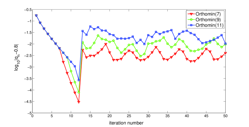
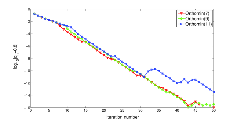
In our attempt to verify Conjecture 3 we conducted numerical experiments with Orthomin($k$) for the system (9) with $U$ as in (14). In Table 2.1 we show the residual norms $|\!|r_{n}^{(k)}|\!|$ as well as the ratios $q_{n}$ for $d=13$, $\rho=0.8$, and $k=1,2,3,4,5,7,9,11$. For $k=5,7,9,11$ we only show iterates 5–14, as the first $4$ iterates are identical to those of Orthomin(4). Note that, in general, the first $k$ steps of Orthomin($k+1$) are identical to those of Orthomin($k$). The numbers in Table 1 show that $q_{n}\to 0.8$ for $k=1,2,3,4,5$, which is confirmed by further examining the difference $|r_{n}-0.8|$. However, for $k=7,9,11$ we notice that $q_{n}$ exhibits an oscillatory behavior and does not appear to converge to $\rho=0.8$. This is confirmed by Figure 1. Further evidence shows that even for $k=7,9,11$ the ratio $q_{n}$ converges to $\rho$ if we increase $d$. This is confirmed in Figure 2. We should point out that we also experimented with random values for $r_{0},b$, as well as small random perturbations $\mu_{k}$ of the numbers $\zeta_{d}^{k}$ (with $\lvert\mu_{k}\rvert=1$): we always observe $q_{n}\to\rho$ as long as $d$ is sufficiently large.

Table 1: Convergence rates for Orthomin($k$) for $d=13,\ \rho=4/5$, $k=1,2,3,4,5,7,9,11$.

it	Orthomin($1$)		Orthomin($2$)		Orthomin($3$)		Orthomin($4$)
	$|\!|r_{n}|\!|$	$q_{n}$	$|\!|r_{n}|\!|$	$q_{n}$	$|\!|r_{n}|\!|$	$q_{n}$	$|\!|r_{n}|\!|$	$q_{n}$
1	3.6056	0.6247	3.6056	0.6247	3.6056	0.6247	3.6056	0.6247
2	2.2524	0.7533	2.2524	0.7156	2.2524	0.7156	2.2524	0.7156
3	1.6967	0.7832	1.6118	0.7768	1.6118	0.7533	1.6118	0.7533
4	1.3289	0.7935	1.2520	0.7919	1.2141	0.7873	1.2141	0.7725
5	1.0544	0.7974	0.9915	0.7958	0.9559	0.7957	0.9379	0.7927
6	0.8407	0.7989	0.7891	0.7985	0.7606	0.7984	0.7435	0.7975
7	0.6717	0.7996	0.6301	0.7993	0.6073	0.7990	0.5929	0.7991
8	0.5371	0.7998	0.5036	0.7997	0.4852	0.7996	0.4738	0.7996
9	0.4296	0.7999	0.4028	0.7999	0.3880	0.7999	0.3789	0.7997
10	0.3436		0.3222		0.3103		0.3030
it	Orthomin($5$)		Orthomin($7$)		Orthomin($9$)		Orthomin($11$)
	$|\!|r_{n}|\!|$	$q_{n}$	$|\!|r_{n}|\!|$	$q_{n}$	$|\!|r_{n}|\!|$	$q_{n}$	$|\!|r_{n}|\!|$	$q_{n}$
5	0.9379	0.7832	0.9379	0.7832	0.9379	0.7832	0.9379	0.7832
6	0.7346	0.7956	0.7346	0.7896	0.7346	0.7896	0.7346	0.7896
7	0.5844	0.7985	0.5800	0.7935	0.5800	0.7935	0.5800	0.7935
8	0.4667	0.7995	0.4602	0.7983	0.4602	0.7959	0.4602	0.7959
9	0.3731	0.7998	0.3674	0.7995	0.3663	0.7974	0.3663	0.7974
10	0.2984	0.7999	0.2937	0.7998	0.2920	0.7993	0.2920	0.7983
11	0.2387	0.7999	0.2349	0.7999	0.2334	0.7998	0.2331	0.7989
12	0.1909	0.8000	0.1879	0.8000	0.1867	0.7999	0.1863	0.7997
13	0.1528	0.7999	0.1503	0.7944	0.1493	0.7882	0.1490	0.7634
14	0.1222		0.1194		0.1177		0.1137

Fig. 1: $\log_{10}|q_{n}-\rho|$ for Orthomin$(k)$, $k=7,9,11$ $(\rho=0.8,\ d=13)$.

Fig. 2: $\log_{10}|q_{n}-\rho|$ for Orthomin$(k)$, $k=7,9,11$ $(\rho=0.8,\ d=32)$.

2.4 Connection with numerical PDEs

Systems of the form (9) arise naturally in the numerical solution of partial differential equations. Consider the steady-state advection-reaction-diffusion equation on $[0,2\pi]$

$$-au^{\prime\prime}(x)+bu^{\prime}(x)+cu(x)=f(x)\ ,\ \ a>0,\ c\geq 0,\ b\in\mathbb{R}\ ,$$ (18)

with periodic boundary conditions $u(0)=u(2\pi),\ u^{\prime}(0)=u^{\prime}(2\pi)$. To obtain a discretization of (18) we proceed as follows: set $x_{j}=jh$, $j=0,1,\dots,d$, $h=2\pi/d$, be a uniform grid (we identify $x_{0}$ with $x_{d}$, $x_{-1}$ with $x_{d-1}$, and $x_{1}$ with $x_{d+1}$), and replace the derivatives in (18) with the usual centered difference formulas

$$-u^{\prime\prime}(x_{j})\approx\frac{2u(x_{j})-u(x_{j-1})-u(x_{j+1})}{h^{2}}\ ,\ \ \ u^{\prime}(x_{j})\approx\frac{u(x_{j+1})-u(x_{j-1})}{2h}\ .$$

The resulting discretization is a linear system of type (1): $A$ is a normal matrix with orthogonal eigenvectors $\chi^{(k)}\in\mathbb{C}^{d}$ and corresponding eigenvalues $\lambda_{k}$ given by

$$\chi^{(k)}_{j}=\exp({\bf i}kjh)\ ,\ \ \lambda_{k}=-\frac{2a}{h^{2}}\cos(kh)+{\bf i}\frac{b}{h}\sin(kh)+c+\frac{2a}{h^{2}}\ .$$

The eigenvalues lie on an ellipse with semi-axes $2a/h^{2}$ and $b/h$; when $2a=hb$ this is a circle of radius $b/h$. After further rescaling, the system can be brought to the form (9). However, as will be shown in Section 3, this example is very relevant to the convergence study of Orthomin$(k)$ also when $2a\neq hb$.

3 Further examples: normal matrices with spectra on ellipses

So far we have examined the systems (9), and we conjectured that for any $k\in\mathbb{N}$ we can find operators $U$ of the form (14) so that for all $1\leq j\leq k$, Orthomin($j$) achieves an asymptotic convergence rate equal to $\rho$. After a trivial rescaling, we restate Conjecture 3 in the following way: for any circle ${\mathcal{C}}$ of center $z_{0}$ and radius $\rho$ satisfying $0<\rho<\lvert z_{0}\rvert$ there exists a normal matrix $A$ whose spectrum lies on ${\mathcal{C}}$ so that for all $1\leq j\leq k$, the Orthomin($j$) iteration applied to the system (1) with $b=(1,1,\dots,1)^{T}$ and zero initial guess has an asymptotic convergence rate of $\rho/\lvert z_{0}\rvert$.

In this section we show numerical evidence suggesting that if we replace the circle ${\mathcal{C}}$ with a non-circular ellipse ${\mathcal{E}}$ in the example above, all Orthomin($j$) with $k\geq 2$ achieve the same asymptotic convergence rate $\rho_{{\mathcal{E}}}$, which is smaller than the asymptotic convergence rate of Orthomin(1). For the exact formulation see Conjecture 5. We remark that the discretized numerical PDE from Section 2.4 is an example of precisely such a system.

In order to make the examples very specific we first describe an ellipse ${\mathcal{E}}$ by its semi-axes $\alpha>0$ and $\beta>0$, the angle $\theta\in\mathbb{R}$ between its axes and the coordinate axes, and the position $u\in\mathbb{C}$ of its center:

$${\mathcal{E}}=\left\{u+e^{{\bf i}\theta}(\alpha\cos\gamma+{\bf i}\beta\sin\gamma)\ :\ \gamma\in[0,2\pi]\right\}\ .$$ (19)

It is assumed that neither ${\mathcal{E}}$ nor its interior contain the origin. For $d\in\mathbb{N}$ we consider the numbers $\mu_{j}\in{\mathcal{E}}$ defined as

$$\mu_{j}=u+e^{{\bf i}\theta}\left(\alpha\cos\frac{2\pi j}{d}+{\bf i}\beta\sin\frac{2\pi j}{d}\right)\ ,\ \ j=1,\dots,d\ .$$ (20)

As before, we associate a linear operator

$$A_{{\mathcal{E}},d}\stackrel{{\scriptstyle\mathrm{def}}}{{=}}\mathrm{diag}[\mu_{1},\dots,\mu_{d}]\ .$$

To construct an analogous continuous-space operator let $d\mu_{{\mathcal{E}}}(z)$ denote the arc-length measure on ${\mathcal{E}}$. Define

$$A_{{\mathcal{E}}}:L^{2}({\mathcal{E}},d\mu_{{\mathcal{E}}})\to L^{2}({\mathcal{E}},d\mu_{{\mathcal{E}}}),\quad A_{{\mathcal{E}}}f(z)=zf(z)\ .$$ (21)

Conjecture 5.

For any ellipse ${\mathcal{E}}$ there exists a number $\rho_{{\mathcal{E}}}\in(0,1)$ so that the following hold:

• For all $k\in\mathbb{N}$ with $k\geq 2$, there exists $d_{k}\in\mathbb{N}$ so that for $d\geq d_{k}$ the ratio $q_{n}=|\!|r_{n+1}^{(k)}|\!|/|\!|r_{n}^{(k)}|\!|$ of the residual-norm obtained by applying the Orthomin$(k)$ iteration with zero initial guess to the system

  $$A_{{\mathcal{E}},d}x=(1,1,\dots,1)^{T}$$ (22)

  satisfies

  $$\lim_{n\to\infty}q_{n}=\rho_{{\mathcal{E}}}\ .$$ (23)

• For any $k\geq 2$ the same ratio obtained by applying the Orthomin$(k)$ iteration with zero initial guess to the continuous system

  $$A_{{\mathcal{E}}}x=1$$

  also satisfies (23).

• If the ellipse is not circular, then $\rho_{{\mathcal{E}}}$ is smaller than the asymptotic convergence rate of Orthomin$(1)$.

Two facts are notable about the behavior of Orthomin$(k)$ on the systems in Conjecture 5. First, it is remarkable that the ratios $q_{n}$ converge at all; indeed, we show that for $k=1$ the sequence $\{q_{n}\}_{n\in\mathbb{N}}$ is convergent regardless of the choice of the numbers $\mu_{1},\dots,\mu_{d}$, but for $k\geq 2$ the sequence $\{q_{n}\}_{n\in\mathbb{N}}$ may not be monotone, and is not expected to converge in general. The second interesting fact is that all Orthomin$(k)$ with $k\geq 2$ achieve the same asymptotic convergence rate for sufficiently large $d$. Moreover, numerical experiments show that $q_{n}$ converges to the same limit $\rho_{{\mathcal{E}}}$ even for a random initial guess and right-hand side $b$. However, in spite of the fact that $\rho_{{\mathcal{E}}}$ seems to be intimately related to the ellipse, currently we do not understand the nature of this connection, i.e., how to compute $\rho_{{\mathcal{E}}}$ using only information about ${\mathcal{E}}$.

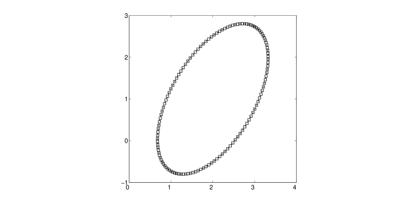
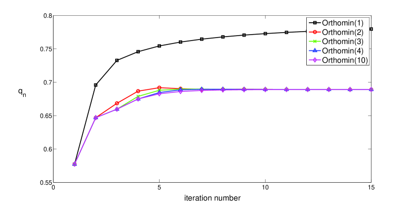
We conclude this section by showing numerical evidence in support of Conjecture 5. For numerical experiments we have selected an ellipse in general position (not aligned with the coordinate axes) with $\alpha=2$, $\beta=1$, $u=2+{\bf i}$, and $\theta=\pi/6$ (see Figure 3). For $d=128$ we solved the system (22) using Orthomin$(k)$ with $k=1,2,3,4,10$. In Figure 4 we plot the ratios $q_{n}$ for each of the solves. The data strongly suggests that for $k=2,3,4,10$ we have

$$q_{n}\to\rho_{{\mathcal{E}}}\approx 0.6891227\ .$$

This approximate value (up to the first eight digits) was also obtained when solving (22) with random right-hand side and initial guess. In the particular case of Orthomin(1), we know that $q_{n}$ is convergent (and monotone increasing): numerically we find that $\lim q_{n}\approx 0.7902$.

Fig. 3: The ellipse with semi-axes $\alpha=2$, $\beta=1$, $u=2+{\bf i}$, and $\theta=\pi/6$ ($d=128$).

Fig. 4: The comparative residual norms for Orthomin(k) ($k=1,2,3,4,5,10$): for Orthomin$(1)$ $q_{n}$ exceeds $0.7902$, but for $k=2,3,4,5,10$ we note a convergence of $q_{n}$ to a value near $0.6891227$.

4 Convergence analysis for Orthomin(1)

The main objective of this section is to prove Conjectures 3 and 4 for $k=1$. In Section 4.1 we show that the sequence $\{q_{n}\}_{n\in\mathbb{N}}$ is increasing and bounded. After stating in Section 4.2 a few technical results, we discuss in Section 4.3 examples when $q_{n}$ does not converge to $\rho$. The behavior of $q_{n}$ for two-dimensional systems is presented in Section 4.4. In Section 4.5 we prove Conjecture 3 for $k=1$. Sections 4.6 and 4.7 are devoted to the infinite-dimensional case (Conjecture 4).

We consider matrices of the form

$$A=\mathop{\operator@font diag}\nolimits[\mu_{1},\dots,\mu_{d}]\ ,$$ (24)

with $\mu_{1},\dots,\mu_{d}\in\mathbb{C}$ nonzero complex numbers. Since we are interested in the evolution of the residuals, we retain only the recursive equation from Orthomin(1) that produces the residual $r_{n}=r_{n}^{(1)}$:

$$r_{n+1}=r_{n}-\Pi_{Ar_{n}}r_{n}\ ,$$ (25)

with $r_{0}\in\mathbb{C}^{d}$ being chosen arbitrarily. Recall from (4) and (6) that

$$\lambda_{n}=\frac{(r_{n},Ar_{n})}{(Ar_{n},Ar_{n})}\ ,\ \ r_{n+1}=r_{n}-\lambda_{n}Ar_{n}\ .$$

Let $r_{n}=(r_{n}^{1},\dots r_{n}^{d})$ be the coefficients of $r_{n}$. We consider the finite probability measure supported at $1,\dots,d$ with weights proportional to $|r_{n}^{1}|^{2}$, …, $|r_{n}^{d}|^{2}$. We will refer to it as the $r_{n}$-measure, and use the subscript $n$ to denote it. For instance, the expected value of a vector $\xi=(\xi_{1},\dots,\xi_{d})$ with respect to this measure is

$$\mathbb{E}_{n}(\xi):=\frac{\sum_{k=1}^{d}\xi_{k}|r_{n}^{k}|^{2}}{\sum_{k=1}^{d}|r_{n}^{k}|^{2}}\ .$$

Since $r_{n+1}=r_{n}-\lambda_{n}Ar_{n}$ has coefficients $r_{n+1}^{k}=(1-\lambda_{n}\mu_{k})r_{n}^{k}$, the following change of variable formula holds:

$$\mathbb{E}_{n+1}(\xi)=\frac{\mathbb{E}_{n}(\xi|1-\lambda_{n}\mu|^{2})}{\mathbb{E}_{n}(|1-\lambda_{n}\mu|^{2})}\ ,$$ (26)

where $\mu=(\mu_{1},\dots,\mu_{d})$ is the vector of eigenvalues of $A$. In particular,

$$\lambda_{n}=\frac{\sum\bar{\mu}_{k}|r_{n}^{k}|^{2}}{\sum|\mu_{k}|^{2}|r_{n}^{k}|^{2}}=\frac{\mathbb{E}_{n}(\bar{\mu})}{\mathbb{E}_{n}(|\mu|^{2})}\ .$$ (27)

4.1 Monotonocity of $q_{n}$

We first show that the sequence $q_{n}$ is increasing and bounded.

Proposition 6.

If $r_{n}$ is given by (25) and $A$ is defined as in (24), then $q_{n}$ is increasing and bounded between $0$ and $1$.

Proof.

We will use the measure-theoretic notation:

$$q_{n}^{2} = \frac{|\!|r_{n+1}|\!|^{2}}{|\!|r_{n}|\!|^{2}}=\mathbb{E}_{n}(|1-\lambda_{n}\mu|^{2})=\mathbb{E}_{n}(1+|\lambda_{n}|^{2}|\mu|^{2}-\lambda_{n}\mu-\bar{\lambda}_{n}\bar{\mu})$$

$$= 1+|\lambda_{n}|^{2}\mathbb{E}_{n}(|\mu|^{2})-\lambda_{n}\mathbb{E}_{n}(\mu)-\bar{\lambda}_{n}\mathbb{E}_{n}(\bar{\mu})\stackrel{{\scriptstyle\eqref{eq:lambdan}}}{{=}}1-\frac{|\mathbb{E}_{n}(\mu)|^{2}}{\mathbb{E}_{n}(|\mu|^{2})}\ .$$

We compare $1-q_{n+1}^{2}$ and $1-q_{n}^{2}$. For the latter, we use the change of variable formula (26):

$$1-q_{n+1}^{2}=\frac{|\mathbb{E}_{n+1}(\mu)|^{2}}{\mathbb{E}_{n+1}(|\mu|^{2})}=\frac{|\mathbb{E}_{n}\left(\mu|1-\lambda_{n}\mu|^{2}\right)|^{2}}{\mathbb{E}_{n}\left(|1-\lambda_{n}\mu|^{2}\right)\mathbb{E}_{n}\left(|\mu|^{2}|1-\lambda_{n}\mu|^{2}\right)}\ .$$

We can re-write this as

$$1-q_{n+1}^{2}=\frac{|\mathbb{E}_{n}(\xi|1-\xi|^{2})|^{2}}{\mathbb{E}_{n}(|1-\xi|^{2})\mathbb{E}_{n}(|\xi|^{2}|1-\xi|^{2})}\ ,$$

with $\xi=\lambda_{n}\mu$. By construction,

$$\mathbb{E}_{n}(\xi)=\mathbb{E}_{n}(|\xi|^{2})=\frac{|\mathbb{E}_{n}(\mu)|^{2}}{\mathbb{E}_{n}(|\mu|^{2})}\ ,$$

hence we can apply the result of Lemma 7 to $\xi$:

$$1-q_{n}^{2}=\mathbb{E}_{n}(|\xi|^{2})\geq\frac{|\mathbb{E}_{n}(\xi|1-\xi|^{2})|^{2}}{\mathbb{E}_{n}(|1-\xi|^{2})\mathbb{E}_{n}(|\xi|^{2}|1-\xi|^{2})}=1-q_{n+1}^{2},$$

hence $q_{n}\leq q_{n+1}$. ∎

Lemma 7.

Let $\xi$ a complex-valued random variable with finite moments up to order $4$ satisfying the identity $\mathbb{E}(\xi)=\mathbb{E}(|\xi|^{2})$. The following inequality then holds:

$$\mathbb{E}(|\xi|^{2})\>\mathbb{E}(|1-\xi|^{2})\>\mathbb{E}(|\xi|^{2}|1-\xi|^{2})\geq|\mathbb{E}(\xi|1-\xi|^{2})|^{2}\ .$$ (28)

Proof. First of all, we remark that if $\xi$ satisfies the condition stated in the Lemma, then so does $1-\xi$. Thus, the situation is symmetric in $\xi$ and $1-\xi$.
Let $\theta\in\mathbb{R}$ such that $\mathbb{E}(\xi|1-\xi|^{2})=e^{i\theta}|\mathbb{E}(\xi|1-\xi|^{2})|$. Consider the function

$$f:\mathbb{R}\to\mathbb{R},\quad f(t):=\operatorname{Var}(t(1-\xi)+e^{i\theta}\bar{\xi}(1-\xi))\ ,$$ (29)

where Var$(\xi)=\mathbb{E}(\lvert\xi\rvert^{2})-\lvert\mathbb{E}(\xi)\rvert^{2}$ denotes the variance of a random variable $\xi$. By opening up the parenthesis inside the expected value, we obtain

$$\begin{split}f(t)&=t^{2}\{\mathbb{E}(|1-\xi|^{2})-|\mathbb{E}(1-\xi)|^{2}\}+2t|\mathbb{E}(\xi|1-\xi|^{2})|+\mathbb{E}(|\xi|^{2}|1-\xi|^{2})\\ &=t^{2}\mathbb{E}(|\xi|^{2})\mathbb{E}(|1-\xi|^{2})+2t|\mathbb{E}(\xi|1-\xi|^{2})|+\mathbb{E}(|\xi|^{2}|1-\xi|^{2}).\end{split}$$

The second equality follows fom a manipulation of the coefficient of $t^{2}$ which takes into account the fact that $\mathbb{E}(\xi)=\mathbb{E}(|\xi|^{2})$. This shows that $f(t)$ is a real valued quadratic form. The fact that it is a positive definite quadratic form follows from the fact that the variance of a random variable is always a positive number. Therefore, $f(t)$ has negative discriminant:

$$|\mathbb{E}(\xi|1-\xi|^{2})|^{2}-\mathbb{E}(|\xi|^{2})\mathbb{E}(|1-\xi|^{2})\mathbb{E}(|\xi|^{2}|1-\xi|^{2})\leq 0\ .\qquad\end@proof$$

We should point out that in the case when $\xi$ is real valued (which is not the case we are dealing with), the statement of Lemma 7 can be reduced to Pearson’s inequality [9] (see also [6]) between the skewness $\tau$ and the kurtosis $\kappa$ of a distribution: $\kappa-\tau^{2}-1\geq 0$. We do not give a proof of this fact, as it is of no relevance to the rest of the paper. Note that we can think of $q_{n}$ as measuring the dispersion of the random variable $\mu$ relative to the $r_{n}$ measure: variance about the mean divided by average size. The monotonicity of $q_{n}$ reflects the fact that $\mu$ becomes increasingly more uniformly distributed relative to the $r_{n}$-measures.

It is important to remark that Proposition 6 holds for all normal (non-singular) matrices since they can be diagonalized using unitary transformations which leave the residual norms of Orthomin($k$), and hence $q_{n}$, unchanged.

4.2 The case $\mu_{k}=1+\rho\zeta_{k}$, $|\zeta_{k}|=1$, and $r_{0}\in\mathbb{C}^{d}$ arbitrary

In this section we assume that $A$ is of the form $A=I+\rho U$, $U=\operatorname{diag}[\zeta_{1},\dots,\zeta_{d}]$, with $0<\rho<1$ and $|\zeta_{1}|=\dots=|\zeta_{d}|=1$. Also, we keep $r_{0}\in\mathbb{C}^{d}$ arbitrary unless otherwise specified. We introduce the following quantities, for $n\geq 0$:

$$\omega_{n}=\frac{(Ur_{n},r_{n})}{(r_{n},r_{n})},\quad T_{n}=\frac{1-\lambda_{n}}{\rho\lambda_{n}}\ .$$ (30)

Note that the coefficients of $r_{n+1}$ are related to those of $r_{n}$ as follows

$$r_{n+1}^{k}=(1-\lambda_{n}\mu_{k})r_{n}^{k}=\rho\lambda_{n}(T_{n}-\zeta_{k})r_{n}^{k},$$ (31)

and the change of variable formula becomes

$$\mathbb{E}_{n+1}(\xi)=\frac{\mathbb{E}_{n}(\xi|T_{n}-\zeta|^{2})}{\mathbb{E}_{n}(|T_{n}-\zeta|^{2})}\ .$$ (32)

Lemma 8.

For $n\geq 0$ we have

$$\lambda_{n}=\frac{1+\rho\bar{\omega}_{n}}{1+\rho^{2}+2\rho I\!\!R\omega_{n}},\quad T_{n}=\frac{\omega_{n}+\rho}{\rho\bar{\omega}_{n}+1},\quad q_{n}^{2}=\rho^{2}\frac{1-|\omega_{n}|^{2}}{1+\rho^{2}+2\rho I\!\!R\omega_{n}}\ ,$$ (33)

where $I\!\!Rz$ denotes the real part of a complex number $z$.

Proof. Let $\zeta=(\zeta_{1},\dots,\zeta_{d})$. Clearly, $\omega_{n}=\mathbb{E}_{n}(\zeta)$. Since $\mu=1+\rho\zeta$, we have

$$\lambda_{n}=\frac{\mathbb{E}_{n}(1+\rho\bar{\zeta})}{\mathbb{E}_{n}(|1+\rho\zeta|^{2})}\ .$$

The formula for $\lambda_{n}$ then follows from the fact that $\mathbb{E}_{n}(1+\rho\bar{\zeta})=1+\rho\bar{\omega}_{n}$, and $\mathbb{E}_{n}(|1+\rho\zeta|^{2})=1+\rho^{2}+2\rho I\!\!R\omega_{n}$. Next, the formula of $T_{n}$ is a direct consequence of the formula of $\lambda_{n}$. Finally,

$$q_{n}^{2} = 1-\frac{|\mathbb{E}_{n}(\mu)|^{2}}{\mathbb{E}_{n}(|\mu|^{2})}=1-\frac{1+\rho^{2}|\omega_{n}|^{2}+2\rho I\!\!R\omega_{n}}{1+\rho^{2}+2\rho I\!\!R\omega_{n}}=\frac{\rho^{2}(1-|\omega_{n}|^{2})}{1+\rho^{2}+2\rho I\!\!R\omega_{n}}\ .\qquad\end@proof$$

Proposition 9.

For $n\geq 0$ we have $|\omega_{n}|\leq 1$ and $0\leq q_{n}\leq\rho$. Moreover, the following statements are equivalent:

$${\bf(a)}\lim_{n\to\infty}q_{n}=\rho\>.\quad{\bf(b)}\lim_{n\to\infty}\omega_{n}=-\rho\>.\quad{\bf(c)}\lim_{n\to\infty}\lambda_{n}=1\>.\quad{\bf(d)}\lim_{n\to\infty}T_{n}=0\>.$$ (34)

Proof.

The bound $|\omega_{n}|\leq 1$ follows from $\|U\|\leq 1$. The fact that $q_{n}$ is increasing has been proved in the previous section, and the bound $q_{n}\leq\rho$ is a direct consequence of Theorem 2. Since $\lambda_{n}$, $T_{n}$, $q_{n}$ are continuous functions of $\omega_{n}$, the statement (b) clearly implies all the others. We also have (a) $\Rightarrow$ (b) since $\frac{1-|\omega|^{2}}{1+\rho^{2}+2\rho I\!\!R\omega}\leq 1$, with equality for $\omega=-\rho$. Similarly (d) $\Rightarrow$ (b) since $T_{n}$ has bounded denominator. Finally

$$1-\lambda_{n}=\frac{\rho(\rho+\omega_{n})}{1+\rho^{2}+2\rho I\!\!R\omega_{n}}\ .$$

Since the denominator is bounded, $\lim_{n}\lambda_{n}=1$ implies $\lim_{n}\omega_{n}=-\rho$ ((c)$\Rightarrow$ (b)). ∎

In addition to the quantities defined above, we also define the higher moments

$$\omega_{n,j}:=\frac{(U^{j}r_{n},r_{n})}{(r_{n},r_{n})}=\mathbb{E}_{n}(\zeta^{j}),\quad j\geq 0\ .$$ (35)

These moments are used in the convergence proof in Section 4.5. Clearly, $\omega_{n,0}=1$ and $\omega_{n,1}=\omega_{n}$. Using the change of variable formula (32),

$$\omega_{n+1,j}=\mathbb{E}_{n+1}(\zeta^{j})=\frac{\mathbb{E}_{n}(\zeta^{j}|T_{n}-\zeta|^{2})}{\mathbb{E}_{n}(|T_{n}-\zeta|^{2})}=\frac{\mathbb{E}_{n}\{\zeta^{j}(1+|T_{n}|^{2}-T_{n}\bar{\zeta}-\bar{T}_{n}\zeta)\}}{\mathbb{E}_{n}\{1+|T_{n}|^{2}-T_{n}\bar{\zeta}-\bar{T}_{n}\zeta\}}\ ,$$

and we obtain the following

Proposition 10.

For $n\geq 0$ we have the following recurrence relation

$$\omega_{n+1,j}=\frac{(1+|T_{n}|^{2})\omega_{n,j}-T_{n}\omega_{n,j-1}-\bar{T}_{n}\omega_{n,j+1}}{1+|T_{n}|^{2}-2I\!\!R(\bar{T}_{n}\omega_{n})},\quad j\geq 1\ .$$ (36)

Corollary 11.

The collection of moments of the initial distribution $\{\omega_{0,j}\}_{j\geq 0}$ completely determine the sequence $\omega_{n}$ and implicitly $q_{n}$.

Note that when $\zeta_{k}$ are the roots of unity of order $d$ we have $\omega_{n,j+d}=\omega_{n,j}$; hence the finite set of initial moments $\{\omega_{0,j}\}_{1\leq j\leq d}$ completely determine the sequence $q_{n}$.

4.3 Non-convergence to $\rho$

Let $\operatorname{Hull}(\zeta_{1},\dots,\zeta_{d})$ denote the convex hull of $\zeta_{1},\dots,\zeta_{d}$. This is a compact convex subset of $\mathbb{C}$. Since

$$\omega_{n}=\frac{\sum_{k=1}^{d}\zeta_{k}|r_{n}(k)|^{2}}{\sum_{k=1}^{d}|r_{n}(k)|^{2}}\in\operatorname{Hull}(\zeta_{1},\dots,\zeta_{d})\ ,$$

the sequence $\omega_{n}$ cannot converge to $-\rho$ unless $-\rho\in\operatorname{Hull}(\zeta_{1},\dots,\zeta_{d})$. Since the statements $\lim_{n}\omega_{n}=-\rho$ and $\lim_{n}q_{n}=\rho$ are equivalent, we have the following.

Proposition 12.

Assume $-\rho\notin\operatorname{Hull}(\zeta_{1},\dots,\zeta_{d})$. Then $\lim_{n}q_{n}\neq\rho$.

Corollary 13.

Assume that $\rho\in(0,1)$ is arbitrary, and $|\theta_{k}|<\pi-\arccos(\rho)$, for $1\leq k\leq d$. If $\zeta_{k}=\exp(i\theta_{k})$, then $\lim q_{n}\neq\rho$.

Proof.

The angles are chosen so that $I\!\!R(\zeta_{k})>\-rho$. This ensures $-\rho\notin\operatorname{Hull}(\zeta_{1},\dots,\zeta_{d})$, and the previous Proposition applies. ∎

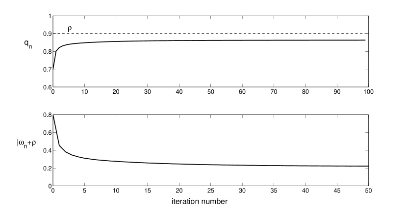
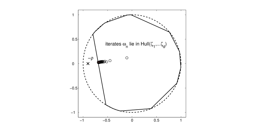
Figures 5 and 6 illustrate the context of Corollary 13: $q_{n}$ does not converge to $\rho$, and $\omega_{n}$ does not converge to $-\rho$. We end this section with a sharpened version of Conjecture 3 for $k=1$:

Conjecture 14.

For Orthomin$(1)$, if $-\rho\in\operatorname{Hull}(\zeta_{1},\dots,\zeta_{d})$, then $q_{n}\to\rho$.

Fig. 5: The case when $-\rho$ does not belong to $\operatorname{Hull}(\zeta_{1},\dots,\zeta_{d})$: $\rho=0.9,\ d=15$.

Fig. 6: The case when $-\rho$ does not belong to $\operatorname{Hull}(\zeta_{1},\dots,\zeta_{d})$: $\rho=0.9,\ d=15$.

4.4 The case d=2

Surprisingly, this case is not completely trivial either.

Proposition 15.

Assume $d=2$ and the initial vector $r_{0}\in\mathbb{C}^{2}$ is arbitrary, with non-zero entries. Then $q_{n}$ is a constant depending on $r_{0}$, while $\omega_{n}$ is a periodic sequence with period $2$. The convergence (15) for $k=1$ does not hold in this case.

Proof.

With a rotation, we may assume $\zeta_{1}=1$ and $\zeta_{2}=\zeta$ is arbitrary. Then $\mu_{1}=1+\rho$ and $\mu_{2}=1+\rho\zeta$. We have

$$\lambda_{0}=\frac{(r_{0},Ar_{0})}{(Ar_{0},Ar_{0})}=\frac{\bar{\mu}_{1}|r_{0}^{1}|^{2}+\bar{\mu}_{2}|r_{0}^{2}|^{2}}{\|Ar_{0}\|^{2}},\quad\omega_{0}=\frac{|r_{0}^{1}|^{2}+\zeta|r_{0}^{2}|^{2}}{|r_{0}^{1}|^{2}+|r_{0}^{2}|^{2}}\ ,$$

therefore

$$1-\lambda_{0}\mu_{1}=\frac{-\rho(1-\zeta)\bar{\mu}_{2}|r_{0}^{2}|^{2}}{\|Ar_{0}\|^{2}}\ ,\qquad 1-\lambda_{0}\mu_{2}=\frac{\rho(1-\zeta)\bar{\mu}_{1}|r_{0}^{1}|^{2}}{\|Ar_{0}\|^{2}}\ .$$

On the other hand $r_{1}=r_{0}-\lambda_{0}Ar_{0}$, hence $r_{1}^{1}=(1-\lambda_{0}\mu_{1})r_{0}^{1}$, and $r_{1}^{2}=(1-\lambda_{0}\mu_{2})r_{0}^{2}$. Therefore

$$\frac{r_{1}^{2}}{r_{1}^{1}}=\frac{1-\lambda_{0}\mu_{2}}{1-\lambda_{0}\mu_{1}}\cdot\frac{r_{0}^{2}}{r_{0}^{1}}=\frac{-\bar{\mu}_{1}|r_{0}^{1}|^{2}}{\bar{\mu}_{2}|r_{0}^{2}|^{2}}\frac{r_{0}^{2}}{r_{0}^{1}}=\frac{-\bar{\mu}_{1}}{\bar{\mu}_{2}}\frac{\bar{r}_{0}^{1}}{\bar{r}_{0}^{2}}\Rightarrow\frac{|r_{1}^{2}|}{|r_{1}^{1}|}=\frac{|\mu_{1}|}{|\mu_{2}|}\frac{|r_{0}^{1}|}{|r_{0}^{2}|}\ .$$ (37)

By applying the same procedure to $r_{1}$ instead of $r_{0}$, we obtain

$$\frac{|r_{2}^{2}|}{|r_{2}^{1}|}=\frac{|r_{0}^{2}|}{|r_{0}^{1}|}\Rightarrow\frac{|r_{2}^{1}|^{2}+\zeta|r_{2}^{2}|^{2}}{|r_{2}^{1}|^{2}+|r_{2}^{2}|^{2}}=\frac{|r_{0}^{1}|^{2}+\zeta|r_{0}^{2}|^{2}}{|r_{0}^{1}|^{2}+|r_{0}^{2}|^{2}},\quad\text{i.e. }\omega_{2}=\omega_{0}\ .$$

This shows that the sequence $\omega_{n}$ is periodic with period $2$. With the above formulae for $1-\lambda\mu_{1}$ and $1-\lambda\mu_{2}$, we also have

$$\frac{\|r_{1}\|^{2}}{\|r_{0}\|^{2}}=\frac{|1-\lambda\mu_{1}|^{2}|r_{0}^{1}|^{2}+|1-\lambda_{1}\mu_{2}|^{2}|r_{0}^{2}|^{2}}{|r_{0}^{1}|^{2}+|r_{0}^{2}|^{2}}=\rho^{2}|1-\zeta|^{2}\frac{|r_{0}^{1}|^{2}|r_{0}^{2}|^{2}}{\|r_{0}\|^{2}\|Ar_{0}\|^{2}}\ .$$ (38)

Let $y=|r_{0}^{2}|^{2}/|r_{0}^{1}|^{2}$. The above fraction equals, up to a constant,

$$\frac{1}{1+1/y}\cdot\frac{1}{1+y|\mu_{2}|^{2}/|\mu_{1}|^{2}}=:g(y)\ .$$

Because of (37), substituting $r_{1}$ for $r_{0}$ amounts to substituting $y$ by $\frac{|\mu_{1}|^{2}}{|\mu_{2}|^{2}}\frac{1}{y}$. This does not change the value of $g(y)$, which means that $\frac{\|r_{2}\|^{2}}{\|r_{1}\|^{2}}=\frac{\|r_{1}\|^{2}}{\|r_{0}\|^{2}}$. This proves that $q_{2}=q_{1}$. Similarly, $q_{n}=q_{n-1}$ for $n\geq 2$. ∎

4.5 Convergence of $q_{n}$ to $\rho$

We have already seen that $\lim_{n}q_{n}=\rho$ if and only if $\lim_{n}\lambda_{n}=1$. In this section we will work with the quantities

$$\beta_{n}:=1-\lambda_{n},\ \ u_{n}:=\omega_{n,1},\ \ \mathrm{and}\ v_{n}:=\omega_{n,2},$$

and we formulate sufficient conditions that guarantee $\beta_{n}\to 0$. We have

$$r_{n+1}=r_{n}-\lambda_{n}(I+\rho U)r_{n}=\beta_{n}Ar_{n}-\rho Ur_{n}\ ,$$ (39)

and

$$(r_{n+1},r_{n+1})=(r_{n+1},r_{n}-\lambda_{n}Ar_{n})=(r_{n+1},r_{n})\ .$$ (40)

Further, since $U$ is unitary,

$$(1-\rho)\leq|\!|A|\!|\leq(1+\rho)\ .$$ (41)

Now,

$$1-\lambda_{n+1} = 1-\frac{(r_{n+1},Ar_{n+1})}{\|Ar_{n+1}\|^{2}}=\rho\frac{(Ur_{n+1},Ar_{n+1})}{\|Ar_{n+1}\|^{2}}$$

$$= \rho\frac{(Ur_{n+1},r_{n+1})+\rho(r_{n+1},r_{n+1})}{\|Ar_{n+1}\|^{2}}=\rho\frac{(Ur_{n+1},r_{n+1})+\rho(r_{n+1},r_{n})}{\|Ar_{n+1}\|^{2}}$$

$$= \rho\frac{(Ur_{n+1},r_{n+1})+(Ur_{n+1},\rho Ur_{n})}{\|Ar_{n+1}\|^{2}}=\rho\frac{(Ur_{n+1},r_{n+1}+\rho Ur_{n})}{\|Ar_{n+1}\|^{2}}$$

$$\stackrel{{\scriptstyle\eqref{eq:resrec}}}{{=}} \rho\frac{(Ur_{n+1},(1-\lambda_{n})Ar_{n})}{\|Ar_{n+1}\|^{2}}=\rho(1-\bar{\lambda}_{n})\frac{(Ur_{n+1},Ar_{n})}{\|Ar_{n+1}\|^{2}}\;.$$

Therefore

$$\beta_{n+1} = \rho\bar{\beta}_{n}\frac{(Ur_{n+1},Ar_{n})}{\|Ar_{n+1}\|^{2}}=\rho\bar{\beta}_{n}\frac{(U(\beta_{n}(I+\rho U)r_{n}-\rho Ur_{n}),(I+\rho U)r_{n})}{\|Ar_{n+1}\|^{2}}$$

$$= \rho\bar{\beta}_{n}\frac{\beta_{n}((U+\rho U^{2})r_{n},(I+\rho U)r_{n})-(\rho U^{2}r_{n},(I+\rho U)r_{n})}{\|Ar_{n+1}\|^{2}}$$

$$= \rho\bar{\beta}_{n}(\beta_{n}((1+\rho^{2})u_{n}+\rho(1+v_{n}))-\rho^{2}u_{n}-\rho v_{n})\frac{\|r_{n}\|^{2}}{\|Ar_{n+1}\|^{2}}\;.$$

Next, the statement

$$\|r_{n+1}\|=\|\beta_{n}Ar_{n}-\rho Ur_{n}\|\geq\rho\|Ur_{n}\|-\|\beta_{n}Ar_{n}\|\geq\|r_{n}\|(\rho-|\beta_{n}|(1+\rho))$$

implies

$$\frac{\|r_{n}\|}{\|Ar_{n+1}\|}=\frac{\|r_{n}\|}{\|r_{n+1}\|}\frac{\|r_{n+1}\|}{\|Ar_{n+1}\|}\leq\frac{1}{(\rho-\lvert\beta_{n}\rvert(1+\rho))(1-\rho)}\ .$$

Therefore

$$|\beta_{n+1}|\leq\rho|\beta_{n}|\frac{(|\beta_{n}|((1+\rho^{2})|u_{n}|+\rho(1+|v_{n}|))+\rho^{2}|u_{n}|+\rho|v_{n}|}{(\rho-|\beta_{n}|(1+\rho))^{2}(1-\rho)^{2}}\ .$$ (42)

Next we need to estimate $\lvert u_{n}\rvert,\lvert v_{n}\rvert$. We have

$$u_{n+1} = \frac{(Ur_{n+1},r_{n+1})}{(r_{n+1},r_{n+1})}=\frac{(U(\beta_{n}Ar_{n}-\rho Ur_{n}),\beta_{n}Ar_{n}-\rho Ur_{n})}{\|r_{n+1}\|^{2}}$$

$$= \frac{|\beta_{n}|^{2}(AUr_{n},Ar_{n})-\rho(\beta_{n}(Ar_{n},r_{n})+\bar{\beta}_{n}(U^{2}r_{n},Ar_{n}))+\rho^{2}(Ur_{n},r_{n})}{\|r_{n+1}\|^{2}}\;,$$

hence

$$|u_{n+1}| = \left(|\beta_{n}|^{2}\|A\|^{2}+2\rho|\beta_{n}|\cdot\|A\|+\rho^{2}|u_{n}|\right)\frac{\|r_{n}\|^{2}}{\|r_{n+1}\|^{2}}$$ (43)

$$\leq \frac{|\beta_{n}|^{2}(1+\rho)^{2}+2\rho|\beta_{n}|(1+\rho)+\rho^{2}|u_{n}|}{(\rho-|\beta_{n}|(1+\rho))^{2}}\,.$$ (44)

The analogous inequality can be derived for $v_{n}$. We summarize the previous inequalities in

Proposition 16.

The following recurrence relations hold:

$$\begin{split}|\beta_{n+1}|&\leq\rho|\beta_{n}|\cdot\frac{|\beta_{n}|[(1+\rho^{2})|u_{n}|+\rho(1+|v_{n}|)]+\rho^{2}|u_{n}|+\rho|v_{n}|}{[\rho-|\beta_{n}|(1+\rho)]^{2}(1-\rho)^{2}}\ ,\\ |u_{n+1}|&\leq\frac{|\beta_{n}|^{2}(1+\rho)^{2}+2\rho|\beta_{n}|(1+\rho)+\rho^{2}|u_{n}|}{(\rho-|\beta_{n}|(1+\rho))^{2}}\ ,\\ |v_{n+1}|&\leq\frac{|\beta_{n}|^{2}(1+\rho)^{2}+2\rho|\beta_{n}|(1+\rho)+\rho^{2}|v_{n}|}{(\rho-|\beta_{n}|(1+\rho))^{2}}\ .\end{split}$$ (45)

We will also need the following inequality which we state without proof.

Lemma 17.

For $|x|\leq 0.1$, $\frac{1}{(1-x)^{2}}\leq 1+Cx$, with $C=2.5$.

Proposition 18.

Assume the following: $0<\rho<0.1$, and $\omega_{0,1}=\omega_{0,2}=\omega_{0,3}=0$. Then, for $n\geq 1$, we have:

1. $|u_{n}|\leq\rho+2.7\sum_{k=2}^{n}\rho^{k}\leq\rho+3\rho^{2}$ ;

2. $|v_{n}|\leq 2.7\sum_{k=2}^{n}\rho^{k}\leq 3\rho^{2}$ ;

3. $|\beta_{n}|\leq\rho^{n+2}$.

Proof.

We use the recurrence relations (36) to compute the first few terms in the sequences $\beta_{n},u_{n},v_{n}$.

$$\begin{split}&T_{0}=\frac{\omega_{0,1}+\rho}{\rho\bar{\omega}_{0,1}+1}=\rho\ ,\quad\beta_{0}=\frac{\rho T_{0}}{1+\rho T_{0}}=\frac{\rho^{2}}{1+\rho^{2}}\ ,\\ &u_{1}=\omega_{1,1}=\frac{(1+|T_{0}|^{2})\omega_{0,1}-T_{0}\bar{\omega}_{0,0}-\bar{T}_{0}\omega_{0,2}}{1+|T_{0}|^{2}-2I\!\!R(\bar{T}_{0}\omega_{0,1})}=\frac{-\rho}{1+\rho^{2}}\ ,\\ &v_{1}=\omega_{1,2}=\frac{(1+|T_{0}|^{2})\omega_{0,2}-T_{0}\bar{\omega}_{0,1}-\bar{T}_{0}\omega_{0,3}}{1+|T_{0}|^{2}-2I\!\!R(\bar{T}_{0}\omega_{0,1})}=0\ ,\\ &T_{1}=\frac{\omega_{1,1}+1}{\rho\bar{\omega}_{1,1}+1}=\rho^{3},\quad\beta_{1}=\frac{\rho T_{1}}{1+\rho T_{1}}=\frac{\rho^{4}}{1+\rho^{4}}\ .\end{split}$$

The inequalities in the proposition are thus true for $n=1$, and we proceed by induction. We assume that the statements (i-iii) are true for some $n\geq 1$, and we prove that they hold for $n+1$ as well. For that, we rely on the inequalities of Proposition 16. We start with the inequality (iii):

$$\begin{split}|\beta_{n+1}|&\leq\rho^{n+3}\times\frac{\rho^{n+2}[(1+\rho^{2})(\rho+3\rho^{2})+\rho(1+3\rho^{2})]+\rho^{2}(\rho+3\rho^{2})+3\rho^{3}}{[\rho-\rho^{n+2}(1+\rho)]^{2}(1-\rho)^{2}}\\ &=\rho^{n+3}\times\frac{\rho^{n+1}[(1+\rho^{2})(1+3\rho)+1+3\rho^{2}]+\rho(1+3\rho)+3\rho}{[1-\rho^{n+1}(1+\rho)]^{2}(1-\rho)^{2}}\\ &\leq\rho^{n+3}\times\frac{\rho^{2}[(1+\rho^{2})(1+3\rho)+1+3\rho^{2}]+\rho(1+3\rho)+3\rho}{[1-\rho^{2}(1+\rho)]^{2}(1-\rho)^{2}}\ .\end{split}$$

The fraction on the right hand side has numerator equal to $4\rho+5\rho^{2}+3\rho^{3}+4\rho^{4}+3\rho^{5}$. This is easily seen to be less than $0.5$, as $0<\rho<0.1$. On the other hand, the denominator is certainly greater than $0.9^{2}\times(1-\frac{1.1}{100})^{2}>0.7$. Therefore the fraction on right hand side is less than $1$, and $|\beta_{n+1}|\leq\rho^{n+3}$.
For inequality (ii),

$$\begin{split}|u_{n+1}|&\leq\frac{\rho^{2(n+2)}(1+\rho)^{2}+2\rho^{n+3}(1+\rho)+\rho^{2}|u_{n}|}{[\rho-\rho^{n+2}(1+\rho)]^{2}}\\ &=\frac{\rho^{2(n+1)}(1+\rho)^{2}+2\rho^{n+1}(1+\rho)+|u_{n}|}{[1-\rho^{n+1}(1+\rho)]^{2}}\\ &=\frac{x^{2}+2x+|u_{n}|}{(1-x)^{2}}\ ,\quad\text{with}\;x=\rho^{n+1}(1+\rho),\\ &\leq(1+Cx)(x^{2}+2x+|u_{n}|)\ ,\quad\text{with}\;C=2.5,\\ &=|u_{n}|+x[2+C|u_{n}|+(2C+1)x+Cx^{2}]\ .\end{split}$$

From the induction step, $|u_{n}|\leq\rho+3\rho^{2}$. Also, $x=\rho^{n+1}(1+\rho)\leq\rho^{2}(1+\rho)$. The quantity inside the square brackets is less than

$$2+C(\rho+3\rho^{2})+(2C+1)\rho^{2}(1+\rho)+C\rho^{4}(1+\rho)^{2}\ .$$

As $0<\rho<1$, this is easily seen to be less than $2.5$. Therefore,

$$|u_{n+1}|\leq|u_{n}|+2.5(1+\rho)\rho^{n+1}<|u_{n}|+2.7\rho^{n+1}\ .$$

Hence $|u_{n+1}|\leq|u_{1}|+2.7\sum_{k=2}^{n+1}\rho^{k}$. The exact same method is applied to $v_{n+1}$. ∎

Theorem 19.

Assume the following hold:

1. $0<\rho<0.1$;

2. $d\geq 4$;

3. $r_{0}=[1,\dots,1]^{T}$;

4. $\zeta_{k}$ are the roots of unity of order $d$;

5. $A=I+\rho U$, $U=diag([\zeta_{1},\dots,\zeta_{d}])$.

Then the sequence $r_{n+1}=r_{n}-\Pi_{Ar_{n}}r_{n}$ satisfies

$$\lim_{n\to\infty}\frac{\|r_{n+1}\|}{\|r_{n}\|}=\rho\ .$$ (46)

Proof. The hypotheses ensure that $\omega_{0,1}=\omega_{0,2}=\omega_{0,3}=0$. Proposition 18 then applies to show

$$\lim_{n}\beta_{n}=0\Rightarrow\lim_{n}\lambda_{n}=1\stackrel{{\scriptstyle(\ref{eq:convequiv})}}{{\Rightarrow}}\lim_{n}q_{n}=\rho\ .\qquad\end@proof$$

4.6 The infinite dimensional case

In this section we prove Conjecture 4 for $k=1$. Recall that $d\mu_{0}$ is the Haar probability measure on the unit circle $\mathbb{S}^{1}$, and assume that $0<\rho<1$ is a fixed parameter (there will be no further restrictions on $\rho$ in this section). For $n\geq 0$, we define

$$\omega_{n}:=\frac{\int_{\mathbb{S}^{1}}zd\mu_{n}(z)}{\int_{\mathbb{S}^{1}}d\mu_{n}(z)},\quad T_{n}:=\frac{\omega_{n}+\rho}{\rho\bar{\omega}_{n}+1},\quad d\mu_{n+1}(z):=|z-T_{n}|^{2}d\mu_{n}(z)\ .$$ (47)

As shown in Section 4.2, the number $\omega_{n}$ is equal to $\left(Ur_{n},r_{n}\right)/\left(r_{n},r_{n}\right)$ where $r_{n}$ is the residual obtained by applying Orthomin(1) to the system (1) with $U$ chosen as in (16), and initial residual $r_{0}\equiv 1$. Our goal is to show that $\lim_{n}T_{n}=0$ which is equivalent to Conjecture 4 for $k=1$. For this, we need the following Lemma.

Lemma 20.

For $q\in\mathbb{C}$ and $n\geq 1$, we define the polynomial in $X$:

$$\Phi_{n}(X,q)=\prod_{k=1}^{n}(X-q^{2k-1})=\sum_{i=0}^{n}a_{i}X^{i}\ ,$$ (48)

where $a_{i}=a_{i}(q)$ are functions of $q$. The following identity holds:

$$\frac{\sum_{i=0}^{n-1}a_{i}a_{i+1}}{\sum_{i=0}^{n}a_{i}^{2}}=\frac{-q(1-q^{2n})}{1-q^{2n+2}}\ .$$ (49)

Proof. This identity can be proved using an identity of MacMahon (see [1, 7]) from the theory of partition functions. We give a few definitions to provide context. The q-Pochhammer symbol is defined as

$$(x;q)_{n}:=\prod_{i=1}^{n}(1-xq^{i-1})\ .$$

When $|q|<1$, the product on the right hand side is convergent as $n\to\infty$, and the limit is denoted by $(x;q)_{\infty}$. The q-binomial coefficient is defined as

$$\left[\begin{array}[]{cc}m\\ n\end{array}\right]_{q}:=\frac{(q;q)_{n}}{(q;q)_{k}(q;q)_{n-k}}\ .$$

MacMahon’s identity ([7], paragraph 323) states that

$$(zq,q)_{m}(z^{-1};q)_{n}=\sum_{k=-n}^{m}(-1)^{k}q^{k(k+1)/2}z^{k}\left[\begin{array}[]{cc}m+n\\ n+k\end{array}\right]_{q}\ .$$ (50)

Using our notation from (48), we note that

$$\Phi_{n}(x,q)\Phi_{n}(1/x,q)=(xq;q^{2})_{n}(x^{-1}q;q^{2})_{n}\ .$$

We apply (50) with $q^{2}$ instead of $q$ and $z=xq^{-1}$, to obtain

$$\Phi_{n}(x,q)\Phi_{n}(1/x,q)=\sum_{k=-n}^{n}(-1)^{k}q^{k^{2}}x^{k}\left[\begin{array}[]{cc}2n\\ n+k\end{array}\right]_{q^{2}}\ .$$ (51)

Identifying the constant coefficient and the coefficient of $x$ on both sides yields

$$\sum_{i=0}^{n}a_{i}^{2}=\left[\begin{array}[]{cc}2n\\ n\end{array}\right]_{q^{2}},\quad\sum_{i=0}^{n-1}a_{i}a_{i+1}=-q\left[\begin{array}[]{cc}2n\\ n+1\end{array}\right]_{q^{2}}\ .$$ (52)

Therefore,

$$\begin{split}\frac{\sum_{i=0}^{n-1}a_{i}a_{i+1}}{\sum_{i=0}^{n}a_{i}^{2}}&=-q\left[\begin{array}[]{cc}2n\\ n+1\end{array}\right]_{q^{2}}/\left[\begin{array}[]{cc}2n\\ n\end{array}\right]_{q^{2}}=-q\frac{(q^{2};q^{2})_{2n}}{(q^{2};q^{2})_{n-1}(q^{2};q^{2})_{n+1}}\frac{(q^{2};q^{2})_{n}^{2}}{(q^{2};q^{2})_{2n}}\\ &=\frac{-q(1-q^{2n})}{1-q^{2n+2}}\ .\qquad\end@proof\end{split}$$

Theorem 21.

Let $\omega_{n}$, $T_{n}$, $\mu_{n}$ be defined by (47). Then $T_{n}=\rho^{2n+1}$, $\forall n\geq 0$. In particular, $\lim_{n}T_{n}=0$, which proves Conjecture 4 for $k=1$.

Proof.

We have

$$\omega_{0}=\frac{\int zd\mu_{0}(z)}{\int d\mu_{0}(z)}=0\ ,\ \ \mathrm{hence}\ T_{0}=\frac{0+\rho}{0\cdot d+1}=\rho\ ,$$

and the statement is true for $n=0$. We proceed by induction. Let $n\geq 1$ and assume that $T_{k}=\rho^{2k+1}$ for $k$ less than $n-1$. From the definition,

$$d\mu_{n}(z)=\prod_{k=0}^{n-1}|z-\rho^{2k+1}|^{2}d\mu_{0}(z)=|\Phi_{n}(z,\rho)|^{2}d\mu_{0}(z)\ .$$ (53)

With $a_{i}=a_{i}(\rho)$, the formula for $\omega_{n}$ reads

$$\omega_{n}=\frac{\int z|\Phi_{n}(z,\rho)|^{2}d\mu_{0}(z)}{\int|\Phi_{n}(z,\rho)|^{2}d\mu_{0}(z)}=\frac{\int z|\sum_{i=0}^{n}a_{i}z^{i}|^{2}d\mu_{0}}{\int|\sum_{i=0}^{n}a_{i}z^{i}|^{2}d\mu_{0}}\ .$$

Since $\int z^{i}d\mu_{0}(z)$ vanishes unless $i=0$, we have

$$\omega_{n}=\frac{\sum_{i,j}a_{i}\bar{a}_{j}\int z^{i+1-j}d\mu_{0}(z)}{\sum_{i,j}a_{i}\bar{a}_{j}\int z^{i-j}d\mu_{0}(z)}=\frac{\sum_{i=0}^{n-1}a_{i}\bar{a}_{i+1}}{\sum_{i=0}^{n}|a_{i}|^{2}}\ .$$ (54)

We can now apply Lemma 20 (note that $a_{i}(\rho)$ are real valued):

$$\omega_{n}=\frac{-\rho(1-\rho^{2n})}{1-\rho^{2n+2}}\ ,\ \ \mathrm{and}\ \ T_{n}=\frac{\omega_{n}+\rho}{\rho\bar{\omega}_{n}+1}=\rho^{2n+2}\ ,$$

which completes the induction step. ∎

Remark. The finite dimensional analogue of Theorem 21 is the case when $d\mu_{0}$ is the equal weighted discrete probability measure supported at the roots of unity of order $d$. The exact same argument works there as well, but only up to $n=d-2$. Beyond that, the right hand side of equation (54) is complicated by the higher correlation sums $\sum_{i}a_{i}a_{i+kd}$, with $k\geq 1$. This is due to the fact that, in the finite dimensional case, the integral $\int z^{n}\mu_{0}(z)=\sum_{k=1}^{d}\exp(\frac{2\pi ink}{d})$ can be nonzero beyond the trivial case $n=0$: namely, when $n\equiv 0\,(\operatorname{mod}d)$. Our proof of Theorem 19 (which allows for some flexibility in the initial conditions) avoided the issue of explicitly computing $T_{n}$.

4.7 Connection with the Jacobi Triple Product Formula

Recall the Jacobi triple product formula ([1], Theorem 2.3) :

$$\prod_{k=1}^{\infty}(1-z\rho^{2k-1})(1-z^{-1}\rho^{2k-1})(1-\rho^{2k})=\sum_{k=-\infty}^{\infty}(-1)^{k}q^{k^{2}}z^{k},\quad|\rho|<1,\;|z|=1\ .$$ (55)

When $|z|=1$ and $\rho\in(0,1)$, this identity can be re-written as

$$\prod_{k=1}^{\infty}|z-\rho^{2k-1}|^{2}=(\rho^{2};\rho^{2})_{\infty}^{-1}\sum_{k\in\mathbb{Z}}(-1)^{k}\rho^{k^{2}}z^{k}\ .$$ (56)

If we compare this to (53) we see that the sequence $d\mu_{n}$ has a strong limit $d\mu_{\infty}$, whose density (with respect to the Haar measure $d\mu_{0}$) is exactly (56).

Recall the quantities $\omega_{n,k}$ defined at (35): in terms of the measures $d\mu_{n}$, they can be written as

$$\omega_{n,k}=\frac{\int_{\mathbb{S}^{1}}z^{k}d\mu_{n}(z)}{\int_{\mathbb{S}^{1}}d\mu_{n}(z)}\ .$$ (57)

We can see now that $\lim_{n}\omega_{n,k}$ can be computed:

$$\lim_{n\to\infty}\omega_{n,k}=\frac{\int_{\mathbb{S}^{1}}z^{k}d\mu_{\infty}(z)}{\int_{\mathbb{S}^{1}}d\mu_{\infty}(z)}=(-1)^{k}\rho^{k^{2}}\ .$$ (58)

Conclusions

For $k\in\mathbb{N}$ we give examples of linear systems (both finite and infinite-dimensional) for which we conjectured that Orthomin(1), $\dots$, Orthomin($k$) achieve the same asymptotic convergence rate. These examples show that, in general, Orthomin($k$) does not converge faster than Orthomin(1). We analyze in detail the convergence of Orthomin(1) and provide numerical evidence in support of our conjectures with respect to Orthomin($k$) for $k>1$. The analysis for Orthomin(1) is fairly complicated and we do not see a straightforward way to extend the arguments to Orthomin($k$) for $k>1$. We provide numerical evidence that certain normal operators (related to numerical PDEs) with spectrum lying on an ellipse, have the following property: Orthomin($2$), Orthomin($3$), etc. all have the same asymptotic convergence rate (depending only on the ellipse); moreover this is smaller than the asymptotic convergence rate of Orthomin($1$). This example offers a promising path to finding improved convergence rate estimates for Orthomin(2) under additional assumptions on the spectrum/field of values of the matrix. An important question, which remains unanswered, is whether there are applications where Orthomin($k$), perhaps coupled with preconditioners, can compete with the usual iterative solvers for non-symmetric systems.

References

- [1] George E. Andrews, The theory of partitions, Addison-Wesley Publishing Co., Reading, Mass.-London-Amsterdam, 1976. Encyclopedia of Mathematics and its Applications, Vol. 2.
- [2] Stanley C. Eisenstat, Howard C. Elman, and Martin H. Schultz, Variational iterative methods for nonsymmetric systems of linear equations, SIAM J. Numer. Anal., 20 (1983), pp. 345–357.
- [3] Howard C. Elman, Iterative methods for large, sparse, nonsymmetric systems of linear equations, PhD thesis, Dept. Computer Science, Yale Univ., New Haven, CT, 1982. Also available as Technical Report 229.
- [4] Anne Greenbaum, Iterative methods for solving linear systems, vol. 17 of Frontiers in Applied Mathematics, Society for Industrial and Applied Mathematics (SIAM), Philadelphia, PA, 1997.
- [5] Karl E. Gustafson and Duggirala K. M. Rao, Numerical range, Universitext, Springer-Verlag, New York, 1997.
- [6] Chris A. J. Klaassen, Philip J. Mokveld, and Bert van Es, Squared skewness minus kurtosis bounded by for unimodal distributions, Statist. Probab. Lett., 50 (2000), pp. 131–135.
- [7] Percy A. MacMahon, Combinatory analysis. Vol. I, II (bound in one volume), Dover Phoenix Editions, Dover Publications Inc., Mineola, NY, 2004. Reprint of An introduction to combinatory analysis (1920) and Combinatory analysis. Vol. I, II (1915, 1916).
- [8] P.K.W. Vinsome, Orthomin, an iterative method for solving sparse sets of simultaneous linear equations, in Proc. of the 4th Symposium on Reservoir Simulation, Society of Petroleum Engineers of AIME, 1976, pp. 149–159.
- [9] J. Ernest Wilkins, Jr., A note on skewness and kurtosis, Ann. Math. Statistics, 15 (1944), pp. 333–335.