Interference competition and invasion: spatial structure, novel weapons and resistance zones

Abstract

Certain invasive plants may rely on interference mechanisms (allelopathy, e.g.) to gain competitive superiority over native species. But expending resources on interference presumably exacts a cost in another life-history trait, so that the significance of interference competition for invasion ecology remains uncertain. We model ecological invasion when combined effects of preemptive and interference competition govern interactions at the neighborhood scale. We consider three cases. Under “novel weapons,” only the initially rare invader exercises interference. For “resistance zones” only the resident species interferes, and finally we take both species as interference competitors. Interference increases the other species’ mortality, opening space for colonization. However, a species exercising greater interference has reduced propagation, which can hinder its colonization of open sites. Interference never enhances a rare invader’s growth in the homogeneously mixing approximation to our model. But interference can significantly increase an invader’s competitiveness, and its growth when rare, if interactions are structured spatially. That is, interference can increase an invader’s success when colonization of open sites depends on local, rather than global, species densities. In contrast, interference enhances the common, resident species’ resistance to invasion independently of spatial structure, unless the propagation-cost is too great. Increases in background mortality (i.e., mortality not due to interference) always reduce the effectiveness of interference competition.

1 Introduction

Both lateral and vertical interactions can affect the likelihood that an invasive species advances when rare (Levine et al., 2004; Going et al., 2009). But for many plants, competitive asymmetry between invader and resident species governs both the outcome and the timescale of ecological invasion (Lavergne and Molofsky, 2004; Vilà and Weiner, 2004; O’Malley et al., 2006a; MacDougall et al., 2009). Given invader-resident competition, ecological superiority may depend on more than one mechanism (Case and Gilpin, 1974; Ridenour and Callaway, 2001). Our analysis addresses the combined impact of preemptive and interference competition on invasion dynamics when biotic interactions are structured spatially. We assume that interference has a cost (Adams et al., 1979; Bazzaz and Grace, 1997; Amarasekare, 2002); an increasing level of interspecific interference requires a reduction in propagation rate, diminishing that species’ capacity to colonize unoccupied sites.

In many plant communities the primary mode of competition is site preemption (Schoener, 1983; Bergelson, 1990; Crawley et al., 1999; Yurkonis and Meiners, 2004); i.e., species interact through colonization of empty sites. Superior preemptive competitors have higher propagation rates or lower mortality rates (Korniss and Caraco, 2005; O’Malley et al., 2006b; Allstadt et al., 2007). The former increases colonization of open sites, and the latter decreases a competitor’s opportunities for colonization. Preemptive competitors have the same niche in a spatially homogeneous environment (Amarasekare, 2003). Ordinarily this precludes coexistence (Shurin et al., 2004; Allstadt et al., 2009), since self-regulation does not exceed interspecific competition. Case and Gilpin (1974) suggest that this niche similarity might favor evolution of interference mechanisms.

An interference competitor inhibits another species’ access to a critical resource, often by harming individuals of the other species. Examples include interspecific territoriality in animals and chemical competition in plants (Case et al., 1994; Callaway and Ascheghoug, 2000). Exotic invaders may suppress native species’ densities through interference competition (D’Antonio and Vitousek, 1992; Callaway and Ridenour, 2004; Cappuccino and Arnason, 2006). The “novel weapons” hypothesis proposes that some invasive plants release chemicals that inhibit growth of native species (Callaway and Ascheghoug, 2000). Interestingly, allelopathic interference may act directly on individuals of the resident competitor, or may act indirectly through toxic effects on native species’ microbial mutualists, particularly mycorrhizal fungi (Wolfe and Klironomos, 2005; Callaway et al., 2008). So, under the novel weapons hypothesis, invaders attain competitive superiority because their phytochemicals present novel challenges to native species. Reasonably, in other communities, exotic species likely encounter interference competition from natives; see comments in Von Holle et al. (2003). Our models address the three general cases where interference can affect the outcome of resident-invader competition. We associate novel weapons with interference by the invader only. We refer to “resistance zones” when the resident species, but not the invader, exerts interference competition. And, of course, invaders and residents may each compete via interference (Case and Gilpin, 1974). If neither species exhibits interference, our model leaves preemption as the sole competitive mechanism. In this case the species that, when alone, maintains the greater equilibrium density will always displace its competitor (Amarasekare, 2003; O’Malley et al., 2006a; Allstadt et al., 2007).

Discrete, stochastic spatial models and their deterministic analogues have been employed, commonly and successfully, to gain insight into collective behavior of multi-“species” interactions (Marro and Dickman, 1999; Murray, 2003) in physics (Korniss et al., 1995, 1997), chemistry (Antal et al., 1996; Toroczkai et al., 1997; Ziff et al., 1986), and in the study of population dynamics (Ellner et al., 1998; McKane and Newman, 2004; O’Malley et al., 2006b, 2009). We use both methods to investigate the combined effects of preemptive and interference competition on invasion. We organize our paper as follows. First, we present a discrete (individual-based), stochastic model where an invader and a resident species compete preemptively, and one or both species also employs interference. We let a species’ propagation rate depend functionally on its level of interference; we consider convex, linear and concave trade-offs. We explore the model by analyzing invasibility criteria of both a mean-field approximation (homogeneous mixing) and a pair approximation. Then we apply results of the approximations to interpret simulations of the full spatial model. The Discussion compares our results to other spatial models incorporating allelopathy. Appendices collect much of the analytical detail.

Our results find that interference by the invader increases its likelihood of successful invasion only when interactions are spatially structured. That is, the novel weapons advantage, in our model, appears only when we account for local clustering of invader individuals. Interference by the resident, the initially common species, can inhibit invasion with and without spatial structure. Increases in background mortality rate (mortality before adjustment due to interference) diminish the competitiveness of the species relying more on interference. Increased mortality reduces both local and global densities; that is, the frequency of empty sites increases. Consequently, the value of interference, relative to propagation, declines. Our model assumes that interference increases mortality of a preemptive competitor, but interference does not generate an alternative niche. Consequently, we should not anticipate coexistence absent continuous introduction or strong effects of spatial clustering (Allstadt et al., 2009).

2 A discrete, stochastic spatial model

When plant species compete, interactions regulating population growth generally occur at the neighborhood scale (Goldberg, 1987; Uriarte et al., 2004). Interference competition, including allelopathy, ordinarily has a local spatial structure. And, when propagule dispersal distance (inter-ramet distance in clonal species) is limited, plants compete preemptively for space at the neighborhood scale. Consequently, our model - which integrates preemptive and interference competition - assumes that competitive interactions among nearest neighbors drive invasion and the dynamics of species’ abundances (O’Malley et al., 2006a).

2.1 Model construction

Two clonal plant species compete on an $L_{x}$ $\times$ $L_{y}$ lattice with periodic boundaries. Each lattice site represents the resources required to sustain a single individual (a ramet) of either species. The local occupation number at site ${\bf x}$ is $n_{i}({\bf{x}})=0,1$ with $i=1,2$, referring to the resident and invader species, respectively. During a single simulated time unit, one Monte Carlo step per site [MCSS], $L_{x}L_{y}$ sites are chosen randomly for updating.

An empty site may be occupied by species $i$ through introduction from outside the environment, or through local propagation. Introduction of species $i$ at an open site occurs as a Poisson process with rate $\beta$. Each species has the same introduction rate, to avert any effect of propagule pressure on the outcome of competition. Local propagation into an open site has rate $\alpha_{i}\eta_{i}({\bf x})$, where $\alpha_{i}$ is the individual-level propagation rate for species $i$, and $\eta_{i}({\bf x})=(1/\delta)\Sigma_{{\bf x}^{\prime}\epsilon{\rm nn}({\bf x})}n_{i}({\bf x}^{\prime})$ is the density of species $i$ in the neighborhood around open site ${\bf x}$. ${\rm{nn}}({\bf x})$ is the set of nearest neighbors of site ${\bf x}$, and $\delta$ is the number of sites in that neighborhood ($\delta=|nn({\bf x})|$). Since we equate colonization with propagation of new ramets, we let $\delta=4$.

Colonization can occur only at open sites. An occupied site opens through mortality. Individuals of each species suffer density-independent mortality at rate $\mu$ (Cain et al., 1995). An individual occupying site x experiences an increased mortality rate due to interference if $nn({\bf x})$ includes any heterospecifics. That is, an individual of species $i$ at site x has total mortality rate $\mu+\theta_{j}\eta_{j}(\textrm{{x}}),~{}i\neq j$. $\theta_{j}\geq 0$ represents interference by species $j$, and $\eta_{j}(\bf x)$ is the density of species $j$ on the neighborhood around site x.

Summarizing transition rules for an arbitrary site ${\bf x}$, we have

$$0\stackrel{{\scriptstyle\beta+\alpha_{1}\eta_{1}(\bf{x})}}{{\longrightarrow}}1,\;\;0\stackrel{{\scriptstyle\beta+\alpha_{2}\eta_{2}(\bf{x})}}{{\longrightarrow}}2,\;\;1\stackrel{{\scriptstyle\mu+\theta_{2}\eta_{2}(\bf{x})}}{{\longrightarrow}}0,\;\;2\stackrel{{\scriptstyle\mu+\theta_{1}\eta_{1}(\bf{x})}}{{\longrightarrow}}0,\;\;$$ (1)

where 0, 1, 2 indicates whether a site is open, resident-occupied, or invader-occupied, respectively. Table 1 defines the symbols and notation we use.

Table 1: Definitions of model variables and parameters

Symbols	Definitions
$L_{x},\;L_{y}(=L)$	Lattice size
x	Location of lattice site
$n_{1}({\bf x})$	Occupation number for residents at site ${\bf x}$; $n_{1}({\bf x})=0,1$
$n_{2}({\bf x})$	Occupation number for invaders at site ${\bf x}$; $n_{2}({\bf x})=0,1$
nn(x)	Set of nearest neighbors around site x
$\delta$	size of neighborhood around site ${\bf x}$ ($\delta=|nn({\bf x})|$)
$\beta$	Common introduction rate at empty sites
$\eta_{i}({\bf x})$	Density of species $i$ on nn(x)
$\alpha_{i}$	Individual rate of propagule production, species $i$
$\mu$	Background mortality rate, both species
$\theta_{j}$	Mortality of species $i$ due to interference by species $j$
$\alpha_{c}(\mu)$	Minimal propagation rate for persistence
$C$	Maximal propagation rate; C = 0.8
$R$	Curvature of $\alpha,\theta$ trade-off
${\rho_{i}}^{*}$	Equilibrium single-species density

We assume that interspecific competition drives the dynamics; i.e., each species persists absent competition. Therefore, we restrict attention to the $\beta\ll\alpha_{c}(\mu)<\alpha_{i}$ $(i=1,2)$ regime, where $\alpha_{c}(\mu)$ is the critical propagation rate below which either species, in the other’s absence, grows too slowly to avoid extinction (Oborny et al., 2005; O’Malley et al., 2006a).

2.2 Life-history constraint

The essential lesson of life-history theory is that increased allocation of resources to one trait advancing survival or reproduction comes at the expense of another trait (Bell and Koufopanou, 1986). Applying this concept, we assume that any increase in a species’ level of interference reduces that species’ clonal propagation rate. The functional dependence (trade-off) has the form $\alpha_{i}^{R}+\theta_{i}^{R}=C^{R}$, where $C$ is a constant, equal to the maximal feasible rate of propagation, and $R$ defines the shape of the trade-off (Giraldeau and Caraco, 2000). If $0<R<1$, the cost of increasing $\alpha$ (i.e., the decrease in $\theta$) decreases as $\alpha$ increases. If $R=1$, the cost of increasing $\alpha$ is constant, and if $R>1$, the cost of increasing $\alpha$ increases at greater $\alpha$. More importantly, any increase in $R$ increases competitiveness of a species that employs both preemption and interference; the constraint moves farther from the origin as $R$ increases. If a species does not exercise interference, we let its propagation rate vary on ($\alpha_{c}(\mu)$, 0.8]. Therefore, we let $C=0.8$.

2.3 Novel weapons

Under the novel weapons hypothesis, the invader exercises interference competition while the resident does not. That is, $\theta_{1}=0$, and

$$0<\theta_{2}\leq\sqrt[R]{C^{R}-{\alpha_{c}(\mu)}^{R}}$$

Invasive plants may interfere with native competitors through several mechanisms. Some impact natives directly; others are mediated through a third species. Invaders can act as a disease reservoir (Eppinga et al., 2006; Borer et al., 2007), focus herbivory on native species (Dangremond et al., 2010), or produce allelopathic chemicals (Prati and Bossdorf, 2004; Cipollini et al., 2008). Our analysis emphasizes the invader’s trade-off between propagation and interference across a range of native species lacking interference. Under the novel weapons hypothesis, the resident species does not compete through interference, and we let its reproductive rate vary to model variation in the strength of preemption the invader encounters.

2.4 Resistance zones

To study resistance zones, we let the resident exercise interference competition while the invader does not. That is, $0<\theta_{1}\leq\sqrt[R]{C^{R}-{\alpha_{c}(\mu)}^{R}}$, and $\theta_{2}=0$. A resident species exercising interference competition may strongly resist invasion since its initial density (by definition) will be relatively high. Given biotic resistance combining preemption and interference, we vary the invader’s propagation rate to consider a range of matches between the invader and the abiotic environment invaded.

2.5 Mutual interference

Under the assumption of mutual interference competition, we have $0<\theta_{1},\theta_{2}\leq\sqrt[R]{C^{R}-{\alpha_{c}(\mu)}^{R}}$. For this case we assume that each species’ resource allocation between propagation and interference follows the same trade-off.

3 Mean-field approximation

The spatially-homogeneous mean-field approximation to our model ignores any effects of locally clustered growth. The mean-field model (MF) so offers comparison to results including interactions at the neighborhood scale; see Wilson (1998), Pascual and Levin (1999) or Cuddington and Yodzis (2000) for perspective.

$\rho_{1}$ and $\rho_{2}$ represent the global densities of species 1 and species 2, respectively. Ignoring continuous introduction (letting $\beta=0$) we have a mean-field dynamics:

$$\dot{\rho_{1}} = \alpha_{1}\rho_{1}(1-\rho_{1}-\rho_{2})-\rho_{1}(\mu+\theta_{2}\rho_{2})$$ (2)

$$\dot{\rho_{2}} = \alpha_{2}\rho_{2}(1-\rho_{1}-\rho_{2})-\rho_{2}(\mu+\theta_{1}\rho_{1})$$ (3)

$\theta_{i}$ represents the increased mortality of species $j$ induced by species $i$; we scale $\theta_{i}$ per unit density of species $i$. Species’ persistence absent competition in the MF approximation requires only that each $\alpha_{i}>\alpha_{c}(\mu)=\mu$. Letting $\theta_{i}\geq 0$, for $i=1,~{}2$, we conduct a general stability analysis of the MF model’s equilibria. Thereafter, we consider competitive superiority when the specific propagation-interference constraint introduced above applies.

3.1 Equilibria and stability

The dynamics has three boundary equilibria and one positive equilibrium. Mutual extinction, designated equilibrium E1, cannot be stable since each $\alpha_{i}>\mu$. At Equilibrium $E2$, species 1 competitively excludes species 2:

$$E2:~{}\left({\rho_{1}}^{*}=1-\frac{\mu}{\alpha_{1}},{\rho_{2}}^{*}=0\right)$$ (4)

Species 2 excludes species 1 at equilibrium $E3$:

$$E3:~{}\left({\rho_{1}}^{*}=0,{\rho_{2}}^{*}=1-\frac{\mu}{\alpha_{2}}\right)$$ (5)

Finally, a positive (internal) equilibrium, $E4$, can be expressed as:

$${\rho_{1}}^{*}=\frac{\theta_{2}(\alpha_{2}-\mu)+\mu(\alpha_{2}-\alpha_{1})}{\alpha_{1}\theta_{1}+\alpha_{2}\theta_{2}+\theta_{1}\theta_{2}}$$ (6)

$${\rho_{2}}^{*}=\frac{\theta_{1}(\alpha_{1}-\mu)+\mu(\alpha_{1}-\alpha_{2})}{\alpha_{1}\theta_{1}+\alpha_{2}\theta_{2}+\theta_{1}\theta_{2}}$$ (7)

As noted above, we know that when competition is strictly preemptive $(\theta_{1}=\theta_{2}=0)$, the species cannot coexist under homogeneous mixing.

Suppose that the resident excludes the invader. From Appendix A, local stability of invader extinction requires:

$$\mu(\frac{\alpha_{2}}{\alpha_{1}}-1)+\theta_{1}(\frac{\mu}{\alpha_{1}}-1)<0$$ (8)

Since $\mu<\alpha_{1}$, $\theta_{1}(\frac{\mu}{\alpha_{1}}-1)\leq 0$. Therefore, any interference by the resident tends to stabilize invader extinction by increasing invader mortality. That is, interference by the common species can help prevent advance of the rare species, even if the rare species has the greater propagation rate. Clearly, if $\alpha_{1}>\alpha_{2}$ and $\theta_{1}\geq 0$, the resident species repels the invader. Note that $\theta_{2}$, the invader’s level of interference competition, does not appear in Inequality (8). Hence the invader cannot increase its growth rate when rare through interference; only increased propagation promotes mean-field invasion.

To elaborate, the invader advances from rarity only if Inequality (8) is reversed. From Appendix A, assuming $\theta_{1}>0$, the rare species invades iff:

$$\alpha_{2}-\alpha_{1}>\theta_{1}(\frac{\alpha_{1}}{\mu}-1)>0$$ (9)

To invade successfully, the rare species must have the greater propagation rate, and must not suffer too much interference from the common species.

Appendix A shows that if species 2 can invade the resident, then equilibrium $E3$ is locally stable. That is, if species 2 can advance when rare, it will grow to exclude species 1.

3.2 Bistability

Bistability requires that local-stability conditions for both single-species equilibrium nodes ($E2$ and $E3$) hold simultaneously. Given bistability, initial conditions determine the outcome; at some point, the more abundant species “wins.” From Appendix A, the common species (1 or 2) repels its rare competitor if

$$\theta_{1}(1-\frac{\alpha_{1}}{\mu})<\alpha_{1}-\alpha_{2}~{}~{}\textrm{and}~{}~{}\theta_{2}(\frac{\alpha_{2}}{\mu}-1)>\alpha_{1}-\alpha_{2}$$ (10)

If $\alpha_{1}>\alpha_{2}$, the first expression must hold, since $\theta_{1}(1-\frac{\alpha_{1}}{\mu})\leq 0$. The second inequality can hold simultaneously if $\theta_{2}$ is relatively large, and the difference between propagation rates is not too large. If $\alpha_{2}>\alpha_{1}$, the second expression must hold, since $\theta_{2}(\frac{\alpha_{2}}{\mu}-1)>0$, and symmetric conditions promoting bistability are clear. Bistability can arise even if the species with the greater propagation rate does not exert interference. For example, if $\alpha_{1}>\alpha_{2}$, the system can be bistable when $\theta_{1}$ = 0 (provided, of course, $\theta_{2}>0$).

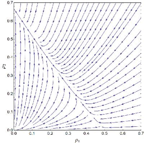
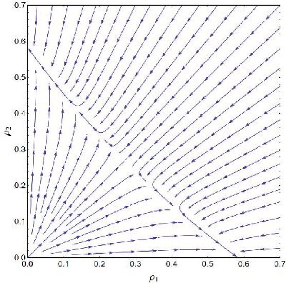
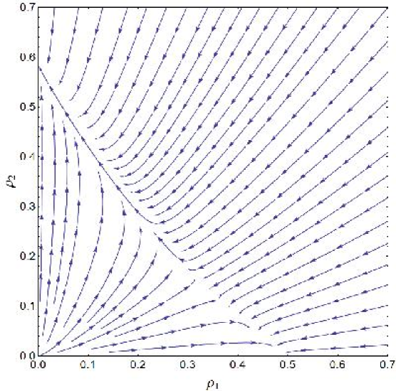
Figure 1 shows how the mean-field dynamics can flow in in the $(\rho_{1},\rho_{2})$ phase space. One example plots competitive asymmetry. Species 2 advances when rare, and when common, excludes species 1. The other plots show bistability, one for a symmetric (identical species), and one for an asymmetric, domain of attraction.

3.3 Coexistence?

Coexistence (local stability of a positive equilibrium) requires that each species invade the other. Together, the conditions for mutual invasion indicate that coexistence requires (Appendix A):

$$\theta_{1}(1-\frac{\alpha_{1}}{\mu})>\alpha_{1}-\alpha_{2}~{}~{}\textrm{and}~{}~{}\theta_{2}(1-\frac{\alpha_{2}}{\mu})>\alpha_{2}-\alpha_{1}$$ (11)

Since each $\alpha_{i}>\mu$, each $(1-\frac{\alpha_{i}}{\mu})<0$; the LHS of each of these inequalities must then be non-positive. But one $(\alpha_{i}-\alpha_{j})$ must be positive, so that the two inequalities cannot be true simultaneously. Hence the MF does not permit mutual invasion, and so does not admit competitive coexistence, when the species interact through both preemption and interference.

3.4 Propagation-interference constraint

The preceding, general stability analyses did not treat interference as a function of propagation rate. Invoking the life-history constraint generates a special case of the MF analysis. The condition for the invader’s advance when rare, Inequality (9), becomes:

$$\alpha_{2}>\alpha_{1}+\Big{(}\frac{\alpha_{1}}{\mu}-1\Big{)}\sqrt[R]{C^{R}-{\alpha_{1}}^{R}}$$ (12)

From the general MF analysis, any allocation to interference by the invader diminishes its propagation rate $(\alpha_{2})$, and so decreases the likelihood of successful invasion. Any increase in $R$, relaxing the propagation-interference tradeoff, increases the range of feasible parameter combinations where the resident repels the invader (see fig. 2). That is, the opportunity for successful invasion declines as $R$ increases in the MF model, since only the resident can benefit from interference under homogeneous mixing.

Increasing background mortality $(\mu)$ increases the likelihood of successful invasion. Greater mortality, with $\theta_{1}$ and the $\alpha_{i}$ fixed, decreases the resident’s density. Consequently, sites available for colonization increase in density, and the impact of interference on the invader’s dynamics declines. Therefore, greater background mortality, which affects both species, decreases the range of feasible parameter combinations where the resident repels the invader (see fig. 2).

If the competitors mix homogeneously, interference can help the resident repel the invader, but cannot promote the rare species’ invasion. Interference, as a mechanism of biotic resistance, has a greater effect when a small level of interference does not cost too much in propagation, and when background mortality is relatively low (so that resident density is relatively high).

4 Pair approximation

Pair approximation (PA) incorporates correlations of the occupation status of nearest neighboring sites into a dynamics (Dickman, 1986; Matsuda et al., 1987; Bauch and Rand, 2000; van Baalen, 2000). By incorporating a minimal spatial structure, PA predicts equilibrium densities of individual-based models more accurately than do MF models (Ellner et al., 1998; Caraco et al., 2001). For our purposes, PA addresses consequences of local clustering, generated by dispersal limitation, for invasion. Appendix B presents details.

The PA tracks global densities $\rho_{i}(t)$, and conditional densities $q_{j|i}(t)$ representing the likelihood that a site is in state ${j}$, given that a neighboring site in state ${i}$ (Sato et al., 2000; O’Malley et al., 2006a). The three global densities ($\rho_{0}(t),\rho_{1}(t),\rho_{2}(t)$) imply 9 local densities (${q_{j|i}}$). However, the PA’s dimension is limited by simple constraints:

$$\rho_{0}+\rho_{1}+\rho_{2}=1$$

$$q_{0|i}+q_{1|i}+q_{2|i}=1$$ (13)

$$q_{i|j}\rho_{j}=q_{j|i}\rho_{i},$$

where $i,j=0,1,2;i\neq j$; we suppress time dependence for simplicity. These constraints leave only 5 of the 12 total variables are independent. Since species 2 is the invader, we track ${\rho_{1},\rho_{2},q_{2|2},q_{1|2},q_{1|1}}$. Note that the dynamics of ${q_{1|2}}$, the conditional density of a resident given an invader at a neighboring site, can depend on a novel-weapons effect when $\theta_{2}>0$.

The dynamics of the global densities, like the mean field approximation, account introduction to empty sites, local propagation, background mortality, and death due to interference competition. For the resident,

$$\dot{\rho}_{1}=\beta\rho_{0}+\rho_{1}\alpha_{1}q_{0|1}-\rho_{1}\mu-\theta_{2}q_{2|1}\rho_{1}\\$$ (14)

Compared to the mean-field model, both local propagation and mortality due to interference depend on local, rather than global, densities. Hence the PA models both site preemption and interference as effects of spatially clustered growth.

To model the dynamics of a local density, we first write the dynamics of a doublet $\rho_{ii}$, a global density, where $\rho_{ii}=\rho_{i}q_{i|i}$. The PA’s doublet dynamics ($d\rho_{ii}/dt$; see Appendix B) introduces the triplets ${q_{2|02}}$ and ${q_{1|22}}$. Ordinary PA assumes that neighbors of neighboring sites are weakly correlated, and lets ${q_{2|02}=q_{2|0}}$ and ${q_{1|22}=q_{1|2}}$. The approximation closes the system of equations, permitting us to write an invasion criterion (Iwasa et al., 1998).

For the invasion analysis, assume that an introduction of species 2 has occurred. Invasion either succeeds or fails before the next introduction event occurs (since $\beta\ll\mu<\alpha_{i}$). Successful invasion requires that the invader have a positive growth rate when rare; $\dot{\rho_{2}}>0$ as $\rho_{2}\rightarrow 0$. From Appendix B, this condition yields the invasion criterion:

$$1-q_{2|2}-q_{1|2}>\frac{\mu+\theta_{1}q_{1|2}}{\alpha_{2}}.$$ (15)

The left side represents the frequency of open sites neighboring an invader, $q_{0|2}$. The right side represents the ratio of death rate to birth rate for the invader. Successful invasion, then, requires that the invader colonize a neighboring, empty site before it dies. The death rate sums background mortality and averaged mortality from the resistance zone about a resident neighboring the invader. The seeming simplicity of the invasion criterion masks an important biological difference between the MF criterion and the neighborhood-scale condition for invasion. In the PA condition for successful invasion, the local density $q_{1|2}$, hence the local density of open sites $q_{0|2}$, depends on $\theta_{2}$, invader interference (see Appendix B). That is, the neighborhood-scale invasion criterion reveals a role for novel weapons, contrasting to the MF result. Consequently, an interfering invader might invade a resident species despite the resident having the greater propagation rate. The right side of the criterion, of course, include the resistance-zone effect of interference by the resident.

To compare the PA invasion criterion to both the MF and simulation of the full spatial model (see below), we evaluated Inequality (15) numerically. We constructed pairwise invasion plots for the three cases defined above: only the invader interferes (novel weapons), only the resident interferes (resistance zones) and both species exercise interference competition. Whenever a species was an interference competitor, we invoked the propagation-interference constraint.

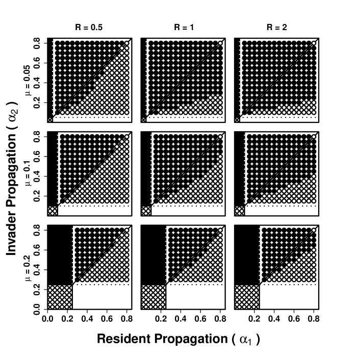
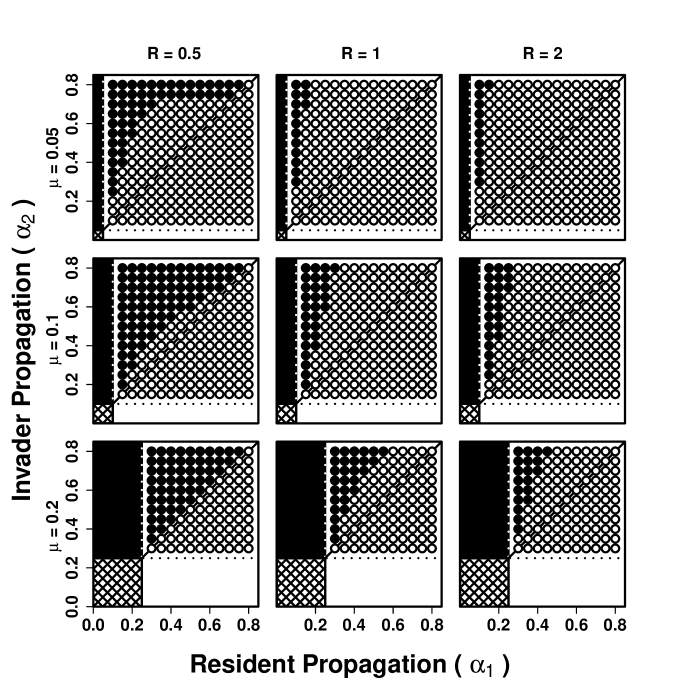
Figure 3 shows pairwise invasion results when the invader, and not the resident, is the interference competitor. That is, the invader obeys the propagation-interference constraint, and $\theta_{1}=0$ independently of the resident’s propagation rate; we so isolate the novel weapons effect. When interactions are local, interference competition can promote an invader’s growth when rare. When the propagation cost of interference is smaller ($R$ is larger) and $\mu$ is small, invaders with a propagation rate much less than the resident’s rate succeed. Invader interference proves advantageous since it opens sites neighboring invaders. Hence interference makes space available where the invader’s local density may match or exceed the resident’s local density - despite the resident’s greater global density. Hence, novel weapons, in our model, enhances invasion when individuals compete at the neighborhood scale, but has no effect under homogeneous mixing.

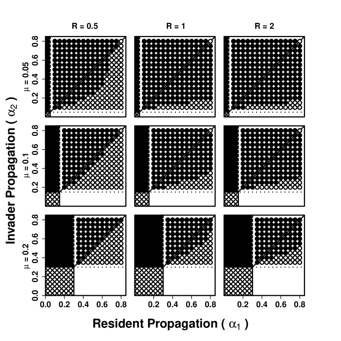
Figure 4 shows pairwise invasion results when the resident, and not the invader, is the interference competitor. That is, the resident obeys the propagation-interference constraint, and $\theta_{2}=0$ independently of the invader’s propagation rate; we isolate the resistance zone effect. A resident can repel an invader with a much higher propagation rate than its own through local interference. Increasing $R$ now reduces the range of parameter combinations permitting invasion, and increasing $\mu$ promotes invader success - results symmetrically opposite to those for novel weapons. When only the resident can interfere, a greater value for $R$ reduces the pleiotropic cost of interference. Increasing $\mu$ opens more space for the invader; greater background mortality renders a given level of interference less effective as a competitive mechanism.

Figure 5 shows pairwise invasion results when both species exercise interference, and so both are constrained by the propagation-interference tradeoff. Not surprisingly, the resident species, because of its initial high density, can employ interference to repel the invader over a much greater range of parameters than when both species lack interference (where greater propagation always wins). The utility of interference, from the resident species’ perspective, declines at small $R$, and at greater $\mu$; the invasion plot for $(R=0.5,\mu=0.2)$ matches the case where competition is strictly preemptive. In most of the plots substantial regions of bistability appear. A species with intermediate levels of both propagation and interference can repel a broad range of propagation-interference combinations. And, when rare, the intermediate combination is repelled by species within that broad range, as long as $R\geq 1$.

Mutual interference does not permit coexistence under PA (fig. 5). In general, the invasion plot resembles the case where only the resident can interfere. But for sufficiently large $R$ and small enough $\mu$, a resident that invests solely in propagation, and not in interference, can be invaded by a species that mixes propagation and interference (rightmost columns of invasion plots). The resident, with an initially high density and no interference capacity, is vulnerable to a clustered invader that can locally open sites via interference competition.

5 Simulation of individual-based model

We simulated the individual-based spatial model with $L_{x}=L_{y}\equiv L=256$, and $\beta$ = 0.001. We initiated simulations with the resident occupying each site. The resident’s density was allowed to decline to its single species equilibrium density, $\rho_{1}^{*}$, without any introduction. Then, at time $t=0$, introduction of both invader and resident individuals began. We tracked the global densities of each species $\rho_{i}(t)$, and recorded a successful invasion when the invader reduced the global density of the resident species to $\rho_{1}^{*}/2$ within 20,000 MCSS time steps. These simulations envision growth of initially small invader clusters at the initiation of ecological invasion (Korniss and Caraco, 2005; O’Malley et al., 2006a; Allstadt et al., 2007).

We can attribute some differences between results of the individual-based spatial model and its pair approximation to the difference in degree of spatial clustering. PA, by construction, truncates correlation length at a nearest neighbors. The simulation model permits development of greater correlation lengths (invader clusters can grow large from a single site). Cluster size impacts the relative frequency at which individuals experience local self-regulation versus interspecific competition (O’Malley et al., 2010). These frequencies, in turn, affect invasion success and global population densities.

We simulated invasion from rare introduction for the three cases examined above: novel weapons, resistance zones, and the case where both species interfere competitively. Figure 6 shows pairwise invasion results when the invader, and not the resident, interferes competitively in the individual-based spatial model. The invader obeys the propagation-interference constraint, and $\theta_{1}=0$ independently of the resident’s propagation rate, isolating the novel weapons effect. Invader interference promotes successful invasion more frequently in simulation than under pair approximation. That is, we note a novel-weapons effect (absent in the MF). Invader clustering increases the advantage of local interference competition against a resident lacking interference. Even when the propagation-cost of interference is steep ($R<1$) an invader may advance and exclude a resident with a greater propagation rate. When interference is less costly ($R>1$) most invaders succeed, except those with a very low propagation rate. PA, then gives a reasonable, but understated, prediction of the impact of novel weapons in the detailed spatial model.

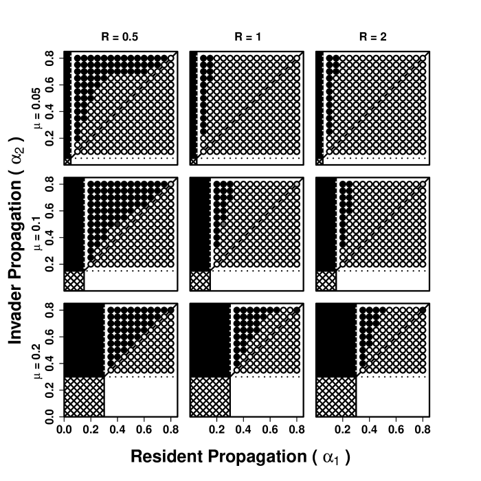
Figure 7 shows pairwise invasion results when the resident, and not the invader, interferes competitively in the individual-based model. The resident obeys the propagation-interference constraint, and $\theta_{2}=0$ independently of the invader’s propagation rate, isolating the resistance zone effect. Interference allows a resident to repel invasion by rare species with much greater rates of local propagation. For the resistance-zone effect, PA predicts the results of the individual-based model very accurately across all parameter combinations we simulated.

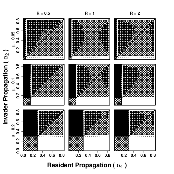
The simulation model’s pairwise invasion results for the case where both species exercise interference competition appear in Figure 8. When the cost of interference is high ($R=0.5$) the results are very close to those for preemptive competition only. That is, the species with the greater rate of propagation wins in most cases. Compared to PA, invader clustering in the simulation model produces more cases of successful invasion at low background mortality. At lesser costs of interference $(R=1,2)$ residents mixing intermediate levels of propagation and interference repel most invading species, particularly when background mortality is not too large. Residents that invest either too much in interference (low $\alpha_{1}$) or too little are susceptible to invasion by species with a more balanced mix of propagation and interference.

In a separate exercise, we released both species from the propagation-interference constraint and searched the parameter space for competitive coexistence. We set $\mu=0.1$, $\beta=0.001$, and let $L=64$ to save computation time. The simulations ran for 100,000 MCSS, and the threshold for coexistence was $\rho_{i}>0.05;i=1,2$, well above the expected density due to introduction alone. The search yielded no evidence of competitive coexistence, as our analytical models predict.

6 Discussion

In the novel weapons scenario an invader gains competitive superiority over a resident through interference. Applications focus on allelopathic interference (Callaway and Ascheghoug, 2000). If species mix homogeneously, we find that a rare invader gains no advantage through interference competition (Case and Gilpin, 1974). But if competitive interactions occur at the local scale, an invader can employ interference to advance against a resident species with a greater rate of local propagation (figs. 3 and 6). Invaders are rare globally but locally clustered in our spatial models. Invaders can use interference to reduce resident density at the perimeter of these clusters, where local invader density is sufficiently high to compete effectively for open sites (Korniss and Caraco, 2005).

In the resistance zone scenario, the resident holds competitive superiority over an invader through interference. A resident’s competitive interference has a strong effect under homogeneous mixing; few invaders advance successfully unless interference is costly and background mortality is high (fig. 2). Under pair approximation, interference by the resident restricts invasion in two cases: when the resident, but not the invader, interferes, and when both species exercise interference competition. The resistance zone effect also appears in simulation of the individual-based model. But when both species can interfere, successful invasion is far more common in the simulation. The difference between the full spatial model and its pair approximation lies in the impact of invader clusters larger than neighborhood size (hence, longer correlation distances) generated by the individual-base model. Clustering increases an invader’s benefit from interference against an interfering resident.

When both species exhibit interference, the pairwise invasion plots indicate regions of bistability (if only one species interferes, one cannot meaningfully reflect invasion plots about the diagonal). We found large regions of bistability under homogeneous mixing. Bistability declined as spatial structure increased (Chao and Levin, 1981), and nearly disappeared in the simulation model (fig. 8). Given a sufficiently long time, we would anticipate that the spatial process on a large, but finite, lattice would result in competitive exclusion. The time required, however, may exceed population-dynamic scales.

In a three-species spatial model, where a non-interfering species interacted with both a weak interferer and a strong interferer, Durrett and Levin (1997) found cyclic coexistence. Our models for two-species competition, by construction, do not admit coexistence. In fact, when we assumed that both species exercise interference competition, and when increased interference reduces propagation, certain parameter sets suggested that a single combination of propagation and interference might repel all other feasible combinations. Suppose we start the resident’s propagation rate, $\alpha_{1}$, at minimal (maximal) levels. Then larger (smaller) propagation rates successively invade and exclude the resident until pairwise competition leaves a resident species that can exclude all others.

Appendix A Mean-field stability

The Jacobian for the spatially homogeneous MF dynamics is:

$$J=\left[\begin{array}[]{cc}\alpha_{1}-\mu-2\alpha_{1}{\rho_{1}}^{*}-{\rho_{2}}^{*}(\alpha_{1}+\theta_{2})&-{\rho_{1}}^{*}(\alpha_{1}+\theta_{2})\\ -{\rho_{2}}^{*}(\alpha_{2}+\theta_{1})&\alpha_{2}-\mu-2\alpha_{2}{\rho_{2}}^{*}-{\rho_{1}}^{*}(\alpha_{2}+\theta_{1})\\ \end{array}\right]$$ (16)

Evaluated at $E1$, mutual extinction, the Jacobian becomes:

$$J(E1)=\left[\begin{array}[]{cc}\alpha_{1}-\mu&0\\ 0&\alpha_{2}-\mu\\ \end{array}\right]$$ (17)

Since $\alpha_{i}>\mu$ for $i=1,~{}2$, by assumption, mutual extinction is unstable.

At $E2$ the resident excludes the invader. The associated Jacobian yields:

$$J(E2)=\left[\begin{array}[]{cc}\alpha_{1}-\mu-2\alpha_{1}(1-\frac{\mu}{\alpha_{1}})&-(1-\frac{\mu}{\alpha_{1}})(\alpha_{1}+\theta_{2})\\ 0&\alpha_{2}-\mu-(1-\frac{\mu}{\alpha_{1}})(\alpha_{2}+\theta_{1})\\ \end{array}\right]$$ (18)

The two eigenvalues are:

$$\lambda_{1}(E2)=\mu(\frac{\alpha_{2}}{\alpha_{1}}-1)+\theta_{1}(\frac{\mu}{\alpha_{1}}-1)$$ (19)

$$\lambda_{2}(E2)=\mu-\alpha_{1}<0$$ (20)

Local stability requires $\lambda_{1}(E2)<0$.

For species 2 to advance when rare, $\lambda_{1}(E2)$ must be positive (implying that extinction of species 2 is unstable). Note that if $\alpha_{2}>\alpha_{1}$ , then $(\frac{\alpha_{2}}{\alpha_{1}}-1)>0$, a condition promoting invasion by species 2 when species 1 rests its single-species equilibrium $E2$. When $\theta_{1}>0$, species 2 invades iff:

$$\alpha_{2}-\alpha_{1}>\theta_{1}(\frac{\alpha_{1}}{\mu}-1)>0$$ (21)

Next, consider $E3$, where species 2 competitively excludes species 1. Evaluating the Jacobian, we have:

$$J(E3)=\left[\begin{array}[]{cc}\alpha_{1}-\mu-(1-\frac{\mu}{\alpha_{2}})(\alpha_{1}+\theta_{2})&0\\ -(1-\frac{\mu}{\alpha_{2}})(\alpha_{2}+\theta_{1})&\alpha_{2}-\mu-2\alpha_{2}(1-\frac{\mu}{\alpha_{2}})\\ \end{array}\right]$$ (22)

The symmetry between $J(E2)$ and $J(E3)$ extends to the eigenvalues. From Eq 22, we obtain:

$$\lambda_{1}(E3)=\mu(\frac{\alpha_{1}}{\alpha_{2}}-1)+\theta_{2}(\frac{\mu}{\alpha_{2}}-1)$$ (23)

$$\lambda_{2}(E3)=\mu-\alpha_{2}<0$$ (24)

Species 2 cannot exclude species 1 iff

$$\alpha_{1}-\alpha_{2}>\theta_{2}(\frac{\alpha_{2}}{\mu}-1)>0$$ (25)

Clearly, reversing subscripts in Expression (9) yields Expression (25). More importantly, we see that if Inequality (9) holds, then $\lambda_{1}(E3)<0$. Hence, if species 2 can invade species 1, $E3$ is the only stable equilibrium, and species 2 advances to exclude species 1 competitively.

Now consider bistability. When common, species 1 repels invasion by species 2 if $\lambda_{1}(E2)<0$. When species 2 is common, it repels invasion by species 1 if $\lambda_{1}(E3)<0$. Both conditions hold, and the dynamics is bistable, iff:

$$\theta_{1}(1-\frac{\alpha_{1}}{\mu})<\alpha_{1}-\alpha_{2}~{}~{}\textrm{and~{}}~{}\theta_{2}(\frac{\alpha_{2}}{\mu}-1)>\alpha_{1}-\alpha_{2}$$ (26)

From our analysis of the single-species equilibria, the two species can coexist iff $\lambda_{1}(E2)>0$ and $\lambda_{1}(E3)>0$. The first inequality implies that when species 1 rests at its single-species equilibrium, species 2 can advance from rarity. The second inequality reverses roles of common and rare. In the text we show that the mean-field dynamics does not admit competitive coexistence.

Appendix B Pair-correlation dynamics

We develop our pair approximation (PA) by modifying methods described by Iwasa et al. (1998). We write a dynamics for five state variables: ${\rho_{1},\rho_{2},q_{2|2},q_{1|2},q_{1|1}}$. The first two are global densities, and the other three are local densities. Invoking constraints listed in the text, Expression (4), we express the remaining PA variables in terms of the five state variables. In particular:

$$\rho_{0}=1-\rho_{1}-\rho_{2}~{}~{}~{}~{}~{}~{}~{}~{}~{}~{}~{}~{}~{}~{}~{}~{}~{}~{}~{}~{}~{}~{}q_{1|0}=\frac{\rho_{1}}{1-\rho_{1}-\rho_{2}}\bigl{(}1-q_{1|1}-q_{1|2}\frac{\rho_{2}}{\rho_{1}}\bigr{)}$$

$$q_{2|0}=\bigl{(}\frac{\rho_{2}}{1-\rho_{1}-\rho_{2}}\bigr{)}(1-q_{2|2}-q_{1|2})~{}~{}~{}~{}~{}~{}~{}~{}~{}~{}~{}~{}~{}~{}~{}~{}~{}~{}~{}q_{0|2}=1-q_{2|2}-q_{1|2}$$

$$q_{0|1}=1-q_{1|1}-q_{1|2}\frac{\rho_{2}}{\rho_{1}}~{}~{}~{}~{}~{}~{}~{}~{}~{}~{}~{}~{}~{}~{}~{}~{}~{}~{}~{}~{}~{}~{}~{}~{}~{}~{}~{}~{}~{}~{}~{}~{}~{}~{}~{}~{}~{}~{}~{}~{}~{}~{}~{}~{}~{}q_{2|1}=q_{1|2}\frac{\rho_{2}}{\rho_{1}}$$

(27)

We omit $q_{0|0}$, also easily calculated, since it does not appear in the analysis.

To begin, we rewrite the dynamics of the resident’s global density, Eq. (14), in terms of our five state variables. Doing the same for the invader’s global density yields:

$$\dot{\rho}_{1}=\beta(1-\rho_{1}-\rho_{2})+\rho_{1}\bigl{[}\alpha_{1}(1-q_{1|1}-q_{1|2}\frac{\rho_{2}}{\rho_{1}})-\mu-\theta_{2}q_{1|2}\frac{\rho_{2}}{\rho_{1}}\bigr{]}$$ (28)

$$\dot{\rho}_{2}=\beta(1-\rho_{1}-\rho_{2})+\rho_{2}\bigl{[}\alpha_{2}(1-q_{2|2}-q_{1|2})-\mu-\theta_{1}q_{1|2}\bigr{]}$$ (29)

To write the dynamics of the three conditional densities, we first require the dynamics of a corresponding doublet. By definition, ${q_{j|i}=\frac{\rho_{ij}}{\rho_{i}}}$, where ${\rho_{ij}}$ is the unordered doublet density. The doublet $\rho_{ij}$ has dynamics:

$$\dot{q}_{j|i}=\frac{1}{\rho_{i}}\dot{\rho}_{ij}-\frac{{q}_{j|i}}{\rho_{i}}\dot{\rho}_{i}$$ (30)

Applying the recipe to ${q_{2|2}}$, we have:

$$\dot{\rho}_{22}=2\rho_{02}\beta+2\rho_{02}\alpha_{2}\Bigl{[}\frac{1}{\delta}+\frac{\delta-1}{\delta}q_{2|02}\Bigr{]}-2\rho_{22}\Bigl{[}\mu+\frac{\delta-1}{\delta}\theta_{1}q_{1|22}\Bigr{]}$$ (31)

The first two terms represent generation of new invader pairs through introduction and birth, and the third term represents the loss of invader pairs due to background mortality and interference competition. This equation introduces triplets ${q_{2|02}}$ and ${q_{1|22}}$ into the dynamics. Ordinary PA takes neighbors of neighboring sites as weakly correlated, and so we assume that $q_{2|02}=q_{2|0}$ and $q_{1|22}=q_{1|2}$. The resulting closure of the equations allows the analysis without including the 27 types of triplets, or any higher order spatial correlations.

Using the closure assumption and converting terms with equation (27), equation (31) becomes

$$\dot{\rho}_{22}=2\rho_{2}(1-q_{2|2}-q_{1|2})\Bigl{[}\beta+\alpha_{2}\bigl{(}\frac{1}{\delta}+\frac{\rho_{2}(\delta-1)}{\delta(1-\rho_{1}-\rho_{2})}(1-q_{2|2}-q_{1|2})\bigr{)}\Bigr{]}$$

$$-2\rho_{2}q_{2|2}\Bigl{[}\mu+\frac{\delta-1}{\delta}\theta_{1}q_{1|2}\Bigr{]}~{}~{}~{}~{}~{}~{}~{}~{}~{}~{}~{}~{}~{}~{}~{}~{}~{}~{}~{}~{}$$ (32)

Substituting Eqq. (14) and (B) into Eq. (30) yields:

$$\dot{q}_{2|2}=2(1-q_{2|2}-q_{1|2})\Bigl{[}\beta+\frac{\alpha_{2}}{\delta}\bigl{(}1+\frac{\rho_{2}(\delta-1)}{1-\rho_{1}-\rho_{2}}(1-q_{2|2}-q_{1|2})\bigr{)}\Bigr{]}$$

$$-q_{2|2}\Bigl{[}\frac{\beta}{\rho_{2}}(1-\rho_{1}-\rho_{2})+\alpha_{2}(1-q_{2|2}-q_{1|2})-\mu-\theta_{1}q_{1|2}\Bigr{]}$$

$$-2q_{2|2}\Bigl{[}\mu+\frac{\delta-1}{\delta}\theta_{1}q_{1|2}\Bigr{]}~{}~{}~{}~{}~{}~{}~{}~{}~{}~{}~{}~{}~{}~{}~{}$$ (33)

Similarly,

$$\dot{q}_{1|1}=2(1-q_{1|1}-q_{1|2}\frac{\rho_{2}}{\rho_{1}})\Bigl{[}\beta+\frac{\alpha_{1}}{\delta}\bigl{(}1+\frac{\rho_{1}(\delta-1)}{1-\rho_{1}-\rho_{2}}(1-q_{1|1}-q_{1|2}\frac{\rho_{2}}{\rho_{1}})\bigr{)}\Bigr{]}$$

$$-q_{1|1}\Bigl{[}\frac{\beta}{\rho_{1}}(1-\rho_{1}-\rho_{2})+\alpha_{1}(1-q_{1|1}-q_{1|2}\frac{\rho_{2}}{\rho_{1}})-\mu-\theta_{2}q_{1|2}\frac{\rho_{2}}{\rho_{1}}\Bigr{]}$$

$$-2q_{1|1}\Bigl{[}\mu+\frac{\delta-1}{\delta}\theta_{2}q_{1|2}\frac{\rho_{2}}{\rho_{1}}\Bigr{]}~{}~{}~{}~{}~{}~{}~{}~{}~{}~{}~{}~{}~{}~{}~{}~{}~{}$$ (34)

${\dot{\rho}_{12}}$ is slightly more complicated. There are two ways to make a (1, 2) pair, and each member of a (1, 2) pair interferes with the other. Proceeding:

$$\dot{\rho}_{12}=\rho_{2}(1-q_{2|2}-q_{1|2})\Bigl{[}\beta+\frac{\alpha_{1}\rho_{1}(\delta-1)}{\delta(1-\rho_{1}-\rho_{2})}(1-q_{1|1}-q_{1|2}\frac{\rho_{2}}{\rho_{1}})\Bigr{]}$$

$$+\rho_{1}(1-q_{1|1}-q_{1|2}\frac{\rho_{2}}{\rho_{1}})\Bigl{[}\beta+\frac{\alpha_{2}\rho_{2}(\delta-1)}{\delta(1-\rho_{1}-\rho_{2})}(1-q_{2|2}-q_{1|2})\Bigr{]}$$

$$-\rho_{2}q_{1|2}\Bigl{[}2\mu+\frac{\theta_{1}}{\delta}\bigl{(}1+(\delta-1)q_{1|2}\bigr{)}+\frac{\theta_{2}}{\delta}\bigl{(}1+(\delta-1)q_{1|2}\frac{\rho_{2}}{\rho_{1}}\bigr{)}\Bigr{]}$$ (35)

Then, following substitution:

$$\dot{q}_{1|2}=(1-q_{2|2}-q_{1|2})\Bigl{[}\beta+\frac{\alpha_{1}\rho_{1}(\delta-1)}{\delta(1-\rho_{1}-\rho_{2})}(1-q_{1|1}-q_{1|2}\frac{\rho_{2}}{\rho_{1}})\Bigr{]}$$

$$+\rho_{1}(1-q_{1|1}-q_{1|2}\frac{\rho_{2}}{\rho_{1}})\Bigl{[}\frac{\beta}{\rho_{2}}+\frac{\alpha_{2}(\delta-1)}{\delta(1-\rho_{1}-\rho_{2})}(1-q_{2|2}-q_{1|2})\Bigr{]}$$

$$-q_{1|2}\Bigl{[}\mu+\frac{\theta_{1}}{\delta}\bigl{(}1+(\delta-1)q_{1|2}\bigr{)}+\frac{\theta_{2}}{\delta}\bigl{(}1+(\delta-1)q_{1|2}\frac{\rho_{2}}{\rho_{1}}\bigr{)}\Bigr{]}$$

$$-q_{1|2}\Bigl{[}\frac{\beta(1-\rho_{1}-\rho_{2})}{\rho_{2}}+\alpha_{2}(1-q_{2|2}-q_{1|2})-q_{1|2}\theta_{1}\Big{]}$$ (36)

Equations (28), (B.3), (B), (B), and (B) constitute the pair-approximation dynamics.

To analyze invasion, we introduce species 2 at near-zero density. Invasion succeeds or fails before the next introduction event occurs (since $\beta\ll\mu_{i}<\alpha_{i}$). Taking $\beta=0$, the PA dynamics becomes:

$$\dot{\rho}_{1}=\rho_{1}\bigl{[}\alpha_{1}(1-q_{1|1}-q_{1|2}\frac{\rho_{2}}{\rho_{1}})-\mu-\theta_{2}q_{1|2}\frac{\rho_{2}}{\rho_{1}}\bigr{]}~{}~{}~{}~{}~{}$$ (37)

$$\dot{\rho}_{2}=\rho_{2}\bigl{[}\alpha_{2}(1-q_{2|2}-q_{1|2})-\mu-\theta_{1}q_{1|2}\bigr{]}~{}~{}~{}~{}~{}$$ (38)

$$\dot{q}_{2|2}=2\alpha_{2}(1-q_{2|2}-q_{1|2})\Bigl{[}\frac{1}{\delta}+\frac{\rho_{2}(\delta-1)}{\delta(1-\rho_{1}-\rho_{2})}(1-q_{2|2}-q_{1|2})\Bigr{]}~{}~{}~{}~{}~{}$$ (39)

$$\quad-q_{2|2}\Bigl{[}\alpha_{2}(1-q_{2|2}-q_{1|2})+\mu+\theta_{1}q_{1|2}\bigl{(}\frac{2(\delta-1)}{\delta}-1\bigr{)}\Bigr{]}~{}~{}~{}~{}~{}$$

$$\dot{q}_{1|1}=2\alpha_{1}(1-q_{1|1}-q_{1|2}\frac{\rho_{2}}{\rho_{1}})\Bigl{[}\frac{1}{\delta}+\frac{\rho_{1}(\delta-1)}{\delta(1-\rho_{1}-\rho_{2})}(1-q_{1|1}-q_{1|2}\frac{\rho_{2}}{\rho_{1}})\Bigr{]}~{}~{}~{}~{}~{}$$ (40)

$$\quad-q_{1|1}\Bigl{[}\alpha_{1}(1-q_{1|1}-q_{1|2}\frac{\rho_{2}}{\rho_{1}})+\mu+\theta_{2}q_{1|2}\frac{\rho_{2}}{\rho_{1}}\bigl{(}\frac{2(\delta-1)}{\delta}-1\bigr{)}\Bigr{]}~{}~{}~{}~{}~{}$$

$$\dot{q}_{1|2}=(1-q_{2|2}-q_{1|2})(1-q_{1|1}-q_{1|2}\frac{\rho_{2}}{\rho_{1}})\bigl{(}\frac{\rho_{1}(\delta-1)}{\delta(1-\rho_{1}-\rho_{2})}\bigr{)}(\alpha_{1}+\alpha_{2})~{}~{}~{}~{}~{}$$ (41)

$$\quad-q_{1|2}\Bigl{[}\mu+\alpha_{2}(1-q_{2|2}-q_{1|2})\Bigr{]}~{}~{}~{}~{}~{}$$

$$-q_{1|2}\Bigl{[}\theta_{1}\bigl{(}\frac{1}{\delta}+\frac{\delta-1}{\delta}q_{1|2}-q_{1|2}\bigr{)}+\theta_{2}\bigl{(}\frac{1}{\delta}+\frac{\delta-1}{\delta}q_{1|2}\frac{\rho_{2}}{\rho_{1}}\bigr{)}\Bigr{]}~{}~{}~{}~{}~{}$$

The next step of the invasion analysis addresses the frequency of open sites when the invader is rare. Since the invader is rare, species 2 has no effect on either the resident’s equilibrium global density ($\rho_{1}^{*}$) or the equilibrium frequency of paired residents ($q_{1|1}^{*})$. Setting $\rho_{2}=0$ in Eqq. (37) and (40) yields:

$$\rho_{1}^{*}=\frac{\delta-1-\frac{\mu}{\alpha_{1}}\delta}{\delta-1-\frac{\mu}{\alpha_{1}}}$$ (42)

and

$$q_{1|1}^{*}=1-\frac{\mu}{\alpha_{1}}.$$ (43)

Now we use these results to find the other conditional probabilities. Let $x=q_{2|2}$, $y=q_{1|2}$, and $w=q_{0|2}=1-x-y$. Then:

$$\dot{x}=\frac{2\alpha_{2}w}{\delta}+xy\theta_{1}\Bigl{[}1-\frac{2(\delta-1)}{\delta}\Bigr{]}-\alpha_{2}wx-\mu x$$

$$\dot{y}=\bigl{(}1-\frac{1}{\delta}-\frac{\mu}{\alpha_{1}}\bigr{)}\bigl{(}\alpha_{1}+\alpha_{2}\bigr{)}w+y\Bigl{[}\alpha_{2}w-\mu-\frac{\theta_{1}}{\delta}-\frac{\theta_{2}}{\delta}\Bigr{]}$$ (44)

$$\qquad+y^{2}\theta_{1}\Bigl{[}1-\frac{\delta-1}{\delta}\Bigl{]}~{}~{}~{}~{}~{}~{}~{}~{}~{}~{}~{}~{}~{}~{}~{}~{}~{}~{}~{}~{}$$

Solving for the equilibria, we have:

$$x^{*}=\frac{2\alpha_{2}w}{\alpha_{2}\delta w+\mu\delta+y^{*}\theta_{1}(\delta-2)}~{}~{}$$

(45)

$$y^{*}=\frac{w(\alpha_{1}+\alpha_{2})(\delta-1-\delta\frac{\mu}{\alpha_{1}})}{\delta\left[\mu+\alpha_{2}w\right]+\theta_{1}-y^{*}\theta_{1}+\theta_{2}}$$ (46)

Given the interdependence of $x^{*}$ and $y^{*}$, we evaluated $(\dot{\rho_{2}})_{\rho_{2}=0}>0$ numerically. Using Eq. (38), we obtain the invasion criterion, Eq. (15) in the text. The importance of deriving $x^{*}$ and $y^{*}$ lies in demonstrating that at the neighborhood scale, both species’ level of interference ($\theta_{1}$ and $\theta_{2}$) affects the likelihood that species 2 can invade the resident species 1. That is, the invasion criterion defined by neighborhood-scale correlations depends not only on the resident’s level of interference $\theta_{1}$ (resistance zone), but on the invader’s level of interference $\theta_{2}$ (novel weapons).

References

- Adams et al. (1979) Adams, J., Kinney, T., Thompson, S., Rubin, L., Helling, R.B. 1979. Frequency-dependent selection for plasmid-containing cells of Escherichia coli. Genetics 91, 627–637.
- Allstadt et al. (2007) Allstadt, A., Caraco, T., Korniss, G. 2007. Ecological invasion: spatial clustering and the critical radius. Evol. Ecol. Res. 9, 1–20.
- Allstadt et al. (2009) Allstadt, A., Caraco, T., Korniss, G. 2009. Preemptive spatial competition under a reproduction-mortality constraint. J. Theor. Biol. 258, 537–549.
- Amarasekare (2002) Amarasekare, P. 2002. Interference competition and species coexistence. Proc. R Soc. Lond. B 269, 2541–2550.
- Amarasekare (2003) Amarasekare, P. 2003. Competitive coexistence in spatially structured environments: a synthesis. Ecol. Let. 6, 1109–1122.
- Antal et al. (1996) Antal, T., Droz, M., Magnin, J., Rácz, Z., Zrinyi, M. 1998. Derivation of the Matalon-Packter law for Liesegang patterns. J. Chem. Phys. 109, 9479–9486.
- Bauch and Rand (2000) Bauch, C., Rand, D.A. 2000. A moment closure model for sexually transmitted disease transmission through a concurrent partnership network. Proc. R. Soc. London B 267, 2019–2027.
- Bazzaz and Grace (1997) Bazzaz, F.A., Grace, J. 1997. Plant resource allocation. Academic Press, San Diego CA.
- Bell and Koufopanou (1986) Bell, G., Koufopanou, V. 1986. The cost of reproduction. Pp. 83–131 in Dawkins, R., Ridley M. (Eds.) Oxford Surveys in Evolutionary Biology:Vol. 3. Oxford University Press, Oxford. UK.
- Bergelson (1990) Bergelson, J. 1990. Life after death: site pre-emption by the remains of Poa annua. Ecology 71, 2157–2165.
- Borer et al. (2007) Borer, E., Hosseini, P., Seabloom, E., Dobson, A. 2007. Pathogen-induced reversal of native dominance in a grassland commuity. Proc. Natl. Acad. Sci. USA 104, 5473–5478.
- Cain et al. (1995) Cain, M.L., Pacala, S.W., Silander Jr., J.A., Fortin, M.-J. 1995. Neighborhood models of clonal growth in the white clover Trifolium repens. Am. Nat. 145, 888–917.
- Callaway and Ascheghoug (2000) Callaway, R.M., Ascheghoug, E.T. 2000. Invasive plants versus their new and old neighbors: a mechanism for exotic invasion. Science 290, 521–523.
- Callaway et al. (2008) Callaway, R.M., Cipollini, D., Barto, K., Thelen, G.C., Hallett, S.G., Prati, D., Stinson, K., Klironomos, J. 2008. Novel weapons: invasive plant suppresses fungal mutualists in America but not in its native Europe. Ecology 89, 1043–1055.
- Callaway and Ridenour (2004) Callaway, R.M., Ridenour, W.M. 2004. Novel weapons: a biochemically based hypothesis for invasive success and the evolution of competitive ability. Front. Ecol. Envir. 2, 436–443.
- Cappuccino and Arnason (2006) Cappuccino, N., Arnason, J.T. 2006. Novel chemistry of invasive exotic plants. Biol. Let. 2, 189–193.
- Caraco et al. (2001) Caraco, T., Duryea, M., Glavanakov, S., Maniatty, W., Szymanski, B.K. 2001. Host spatial heterogeneity and the spread of vector-borne infection. Theor. Pop. Biol. 59, 185–206.
- Case et al. (1994) Case, T.J., Bolger, D.T., Petren, K. 1994. Invasions and competitive displacement among house geckos in the tropical Pacific. Ecology 75, 464–477.
- Case and Gilpin (1974) Case, T.J., Gilpin, M.E. 1974. Interference competition and niche theory. Proc. Natl. Acad. Sci. USA 71, 3073–3077.
- Chao and Levin (1981) Chao, L., Levin, B.R. 1981. Structured habitats and the evolution of anticompetitor toxins in bacteria. Proc. Natl. Acad. Sci. USA 78, 6324–6328.
- Cipollini et al. (2008) Cipolllini, D., Stevenson, R., Cipolllini, K. 2008. Contrasting effects of allelochemicals from two invasive plants on the performance of a nonmycorrhizal plant. Intl. J. Plant Sci. 169, 371–375.
- Connolly and Muko (2003) Connolly, S.R., Muko, S. 2003. Space preemption, size-dependent competition and the coexistence of clonal growth forms. Ecology 84, 2979–2988.
- Crawley et al. (1999) Crawley, M.J., Brown, S.I., Heard, M.S., Edwards, G.R. 1999. Invasion-resistance in experimental grassland communities: species richness or species identity? Ecol. Let. 2, 140–148.
- Cuddington and Yodzis (2000) Cuddington, K.M., Yodzis, P. 2000. Diffusion-limited predator-prey dynamics in Euclidian environments: an allometric individual-based model. Theor. Pop. Biol. 58, 259–278.
- Dangremond et al. (2010) Dangremond, E., Pardini, E., Knight, T. 2010. Apparent competition with an invasive plant hastens the extiction of an endangered lupine. Ecology 91, 2261–2271.
- DAntonio (1993) D’Antonio, C. M. 1993. Mechanisms controlling invasion of coastal plant communities by the alien succulent Carpobrotus edulis. Ecology 74, 83–95.
- D’Antonio and Vitousek (1992) D’Antonio, C.M., Vitousek, P.M. 1992. Biological invasions by exotic grasses, the grass/fire cycle, and global change. Annu. Rev. Ecol. Syst. 23, 63–87.
- Dickman (1986) Dickman, R. 1986. Kinetic phase transitions in a surface-reaction model: mean-field theory. Phys. Rev. A 34, 4246-4250.
- Durrett and Levin (1997) Durrett, R., Levin, S.A. 1997. Allelopathy in spatially distributed populations. J. Theor. Biol. 185, 165–171.
- Ellner et al. (1998) Ellner, S., Sasaki, A., Haraguchi, Y., Matsuda, H. 1998. Speed of invasion in lattice population models: pair-edge approximation. J. Math. Biol. 36, 469–484.
- Eppinga et al. (2006) Eppinga, M., Rietkerk, M., Dekker, S., De Ruiter, P., Van der Putten, W. 2006. Accumulation of local pathogens: a new hypothesis to explain exotic plant invasions. Oikos 114, 168–176.
- Giraldeau and Caraco (2000) Giraldeau, L.-A., Caraco, T. 2000. Social foraging theory. Princeton University Press, Princeton NJ.
- Going et al. (2009) Going, B.M., Hillerislambers, J., Levine, J.M. 2009. Abiotic and biotic resistance to grass invasion in serpentine annual plant communities. Oecologia 159, 839–847.
- Goldberg (1987) Goldberg, D.E. 1987. Neighborhood competition in an old-field plant community. Ecology 68, 1211–1223.
- Iwasa et al. (1998) Iwasa, Y., Nakamuru, M., Levin, S. 1998. Allelopathy of bacteria in a lattice population: competition between colicin-sensitive and colicin-producing strains. Evol. Ecol. 12, 785–802.
- Kisdi and Geritz (2003) Kisdi, E., Geritz, S. 2003. On the coexistence of perennial plants by the competition-colonization trade-off. Am. Nat. 161:350–354.
- Korniss and Caraco (2005) Korniss, G., Caraco, T. 2005. Spatial dynamics of invasion: the geometry of introduced species. J. Theor. Biol 233, 137–150.
- Korniss et al. (1995) Korniss, G., Schmittmann, B., Zia, R.K.P. 1995. Novel phase transitions in biased diffusion of two species. Europhys. Lett. 32, 49–54.
- Korniss et al. (1997) Korniss, G., Schmittmann, B., Zia, R.K.P. 1997. Nonequilibrium phase transitions in a simple three-state lattice gas. J. Stat. Phys. 86, 721–748.
- Lavergne and Molofsky (2004) Lavergne, S., Molofsky, J. 2004. Reed canary grass (Phalaris arundinacea) as a biological model in the study of plant invasions. Crit. Rev. Plant Sci. 23, 415–429.
- Levine et al. (2004) Levine, J.M., Adler, P.B., Yelenik, S.G. 2004. A meta-analysis of biotic resistance to exotic plant invasions. Ecol. Let. 7, 975–989.
- Levine and Rees (2002) Levine, J.M., Rees, M. 2002. Coexistnce and relative abundance in annual plant assemblages: the roles of competition and colonization. Am. Nat. 160, 452–467.
- MacDougall et al. (2009) MacDougall, A.S., Gilbert, B., Levine, J.M. 2009. Plant invasions and the niche. J. Ecology 97, 609–615.
- Marro and Dickman (1999) Marro, J., Dickman, R. 1999. Nonequilibrium phase transitions in lattice models. Cambridge University Press, Cambridge, UK.
- Matsuda et al. (1987) Matsuda, H., Tamachi, N. Ogita, A., Sasaki, A. 1987. A lattice model for population biology. In: Teramoto E., Yamaguti, M. (Eds.), Mathematical Topics in Biology: Lecture Notes in Biomathematics, Volume 71. Springer, New York, pp. 154-161.
- McKane and Newman (2004) McKane, A.J., Newman, T.J. 2004. Stochastic models in population biology and their deterministic analogues. Phys. Rev. E 70, 041902.
- Murray (2003) Murray, J.D., 2003. Mathematical biology, vols. I. and II. 3rd ed. Springer, New York.
- Oborny et al. (2005) Oborny, B., Meszéna, G., Szabó, G. 2005. Dynamics of populations on the verge of extinction. Oikos 109, 291–296.
- O’Malley et al. (2006a) O’Malley, L., Basham, J., Yasi, J.A., Korniss, G., Allstadt, A., Caraco, T. 2006a. Invasive advance of an advantageous mutation: nucleation theory. Theor. Pop. Biol. 70, 464–478.
- O’Malley et al. (2009) O’Malley, L., Korniss, G., Caraco, T. 2009. Ecological invasion, roughened fronts, and a competitor’s extreme advance: integrating stochastic spatial-growth models. Bull. Math. Biol. 71, 1160–1188.
- O’Malley et al. (2010) O’Malley, L., Korniss, G., Mungara, S.S.P., Caraco, T. 2010. Spatial competition and the dynamics of rarity in a temporally varying environment. Evolu. Ecol. Res. 12, 279–305.
- O’Malley et al. (2006b) O’Malley, L., Kozma, B., Korniss, G., Rácz, Z., Caraco, T. 2006b. Fisher waves and front propagation in a two-species invasion model with preemptive competition. Phys. Rev. E 74: 041116, 7 p.
- Pascual and Levin (1999) Pascual, M., Levin, S.A. 1999. From individuals to population densitites: searching for the intermediate scale of nontrivial determinism. Ecology 80, 2225–2236.
- Prati and Bossdorf (2004) Prati, D., Bossdorf, O. 2004. Allelopathic inhibition of germination by Alliaria petiolata (Brassicaceae). Am. J. Botany 91, 285–288.
- Ridenour and Callaway (2001) Ridenour, W., Callaway, R. 2001. The relative importance of allelopathy in interference: the effects of an invasive weed on a native bunchgrass. Oecologia 126, 444- 450.
- Sato et al. (2000) Sato, K., Iwasa, Y. 2000. Pair approximations for lattice-based ecological models. In: Dieckmann, U., Law, R. Metz, J.A.J. (Eds.), The Geometry of Ecological Interactions. Cambridge University Press, Cambridge, pp. 341-358.
- Schoener (1983) Schoener, T. 1983. Field experiments on interspecific competition. Am. Nat. 122, 240–285.
- Schwinning and Parsons (1996) Schwinning, S., Parsons, A.J. 1996. A spatially explicit population model of stoloniferous N-fixing legumes in mixed pasture with grass. J. Ecology 84, 815–826.
- Shurin et al. (2004) Shurin, J.B., Amarasekare, P., Chase, J.M., Holt, R.D., Hoopes, M.F., Leibold, M.A. 2004. Alternative stable states and regional community structure. J. Theor. Biol. 227, 359–368.
- Toroczkai et al. (1997) Toroczkai, Z., Korniss, G., Schmittmann, B., Zia, R.K.P. 1997. Brownian–vacancy -mediated disordering dynamics. Europhys. Lett. 40, 281–286.
- Uriarte et al. (2004) Uriarte, M., Condit, R., Canham, C.D., Hubbell, S.P. 2004. A spatially explicit model of sapling growth in a tropical forest: does the identity of neighbours matter? J. Ecology 92, 348–360.
- van Baalen (2000) van Baalen, M. 2000. Pair approximations for different spatial geometries. In: Dieckmann, U., Law, R. Metz, J.A.J. (Eds.) The Geometry of Ecological Interactions. Cambridge University Press, Cambridge, pp. 359-387.
- Vilà and Weiner (2004) Vilà, M., Weiner, J. 2004. Are invasive plant species better competitors than native plant species? - evidence from pair-wise experiments. Oikos 105, 229–238.
- Von Holle et al. (2003) Von Holle, B., Delcourt, H.R., Simberloff, D. 2003. The importance of biological inertia in plant community resistance to invasion. J. Veg. Sci. 14:425–432.
- Wilson (1998) Wilson, W. 1998. Resolving discrepancies between deterministic population models and individual-based simulations. Am. Nat. 151, 116–134.
- Wolfe and Klironomos (2005) Wolfe, B.E., Klironomos, J.N. 2005. Breaking new ground: soil communities and exotic plant invasions. BioSci. 55, 488–487.
- Yurkonis and Meiners (2004) Yurkonis, K.A., Meiners, S.J. 2004. Invasion impacts local species turnover in a successional ecosystem. Ecol. Let. 7, 764–769.
- Ziff et al. (1986) Ziff, R.M., Gulari, E., Barshad, Y. 1986. Kinetic phase transitions in an irreversible surface-reaction model. Phys. Rev. Lett. 56, 2553 -2556.