The role of the indirect tunneling processes and asymmetry in couplings in orbital Kondo transport through double quantum dots

Abstract

System of two quantum dots attached to external electrodes is considered theoretically in orbital Kondo regime. In general, the double dot system is coupled via both Coulomb interaction and direct hoping. Moreover, the indirect hopping processes between the dots (through the leads) are also taken into account. To investigate system’s electronic properties we apply slave-boson mean field (SBMF) technique. With help of the SBMF approach the local density of states for both dots and the transmission (as well as linear and differencial conductance) is calculated. We show that Dicke- and Fano-like line shape may emerge in transport characteristics of the double dot system. Moreover, we observed that these modified Kondo resonances are very susceptible to the change of the indirect coupling’s strength. We have also shown that the Kondo temperature become suppressed with increasing asymmetry in the dot-lead couplings when there is no indirect coupling. Moreover, when the indirect coupling is turned on the Kondo temperature becomes suppressed. By allowing a relative sign of the nondiagonal elements of the coupling matrix with left and right electrode, we extend our investigations become more generic. Finally, we have also included the level renormalization effects due to indirect tunneling, which in most papers is not taken into account.

I Introduction

Originally, Kondo effect was discovered in non-magnetic metal containing magnetic impurities at low temperature. The effect comes from strong electron correlations and can be regarded as interactions of the impurity spin with cloud of the conduction electrons in metal. Scattering of the conduction electrons from the localized magnetic impurities leads to increase of the resistivity at low temperature. Kondo In recent two decades one could notice revival of this effect as it was predicted and observed in transport through quantum dots. cronewett ; gores ; glazman Although, in this case Kondo resonance leads to increasing conductivity (not resistivity as in original Kondo effect) with decreasing temperature below so-called Kondo temperature $T_{K}$, the physical mechanism of the phenomena is common. Here, the role of the magnetic impurity plays a spin on the dot.

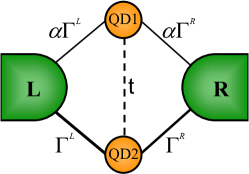
Figure 1: Schematic picture of the double dot system. The parameter $\alpha$ takes into account difference in the coupling of the two dots to external leads ($\alpha\in\langle 0,1\rangle$). Tuning parameter $\alpha$ one can change geometry of the system from the parallel one for $\alpha=1$ to the T-shaped geometry for $\alpha=0$.

However, despite of regarding spin degree of freedom one may assume any two-valued quantum numbers, as for instance, an orbital degree of freedom, to realize Kondo effect. In the case of (at least) two discrete orbital levels coupled to the external leads one may deal with orbital Kondo effect. zawadowski ; boese ; imry To explain mechanism of creation of the Kondo state let us introduce spinless electrons in a system of two single-level quantum dots coupled to external leads as shown in Fig. 1. The dots’ energy levels are well below the Fermi level of the leads. Due to large interdot Coulomb repulsion only one of them is occupied by an electron. On the other hand, removing an existing electron on the double dot requires adding energy to the system. Thus, the system is in the deep Coulomb blockade and the sequential tunneling events are prohibited. However, according to the Heisenberg uncertainty principle, the higher-order processes, however, may appear on a very short time scale. Assuming that initially the upper dot was occupied, then it can tunnel onto the Fermi level of the lead (left or right) and simultaneously another electron from the Fermi level of the left or right electrode may tunnel to the lower dot. As a result, the charge exchange occured between the dots. A coherent superpostion of such coherent events give rise to the sharp resonance in the density of states at the Fermi level.

Altough orbital Kondo effect has been investigated in different geometries of the two orbital level system both experimentally wilhelm ; hubel and theoretically sunG ; sztenkiel ; sztenkiel2 ; holle ; krychowski ; schon there is a little comprehensive studies on the influence of the indirect coupling and/or asymmetry couplings on this phenomenon. In the case of spin Kondo effect most of researchers assume the maximal value of this coupling. vernekPE ; delftPRB05 ; lopezPRB05 ; konikPRL07 ; zhangPRB05 ; ding ; tanakaPRB However, the maximal value of the indirect coupling in the case of the orbital Kondo effect may leads to suppression of Kondo resonance. Specifically, this effect is destroyed when the magnetic flux achieves $2n\pi$ ($n\in\mathbb{Z}$) wen ; kubo08 due to the formation of the bound state in the continuum (BIC) bic . Recently, Kubo et al. have investigated both spin and orbital Kondo effect in double quantum dot regarding non-maximal values of the indirect coupling kubo08 ; kubo11 . They have found that in the condition of intermediate indirect coupling strength the differential conductance reveals two kinds of peaks. Altough, we considered similar system, the role of this paper is to give more insight into the connection between the role of the indirect coupling and various interference effects. Moreover, we assume different asymmetry coupling of the dots to the external leads. More specifically, in the system considered here one dot is coupled to the leads with constant strength, whereas the coupling of the second dot to the leads can be continuously tuned. Time reversal symmetry implies that the amplitude of the indirect coupling strength may change sign gurvitz . Thus, we also include this case in our consideration.

In very recent experiment Tarucha et al. taruchaPRL11 observed that the period of the Aharonov-Bohm oscillations are halved and the phase changes by half a period for the antibonding state from those of the bonding. They conclude that these features can be related to the indirect interdot coupling via the two electrodes.

We also point out that similar double dot system has been investigated in Refs. [medenPRL06, ; medenPRL09, ] where the authors have found a novel pair of correlation-induced resonances as well as they studied the charging of a narrow QD level capacitively coupled to a broad one. However, the correlation-induced effects are not related to the Kondo physics.

As we mentioned before various quantum interference effects, which were previously reported in atomic physics or quantum optics dicke1 ; dicke2 ; Fano , were also discovered in electronic transmission through QDs systems attached to the leadsguevaraD ; shahbazyan ; brandes ; trocha ; trocha1 . Here, we consider Dicke and Fano resonances. In original Dicke effect one observes in spontaneous emission spectra a strong and very narrow resonance which coexist with much broader line. This occurs when the distance between the atoms is much smaller than the wavelength of the emitted light (by individual atom). The former resonance, associated with a state which is weakly coupled to the electromagnetic field, is called subradiant mode, and the latter, strongly coupled to the electromagnetic field refers to superradiant mode. In the case of electronic transport in mesoscopic systems (for instance, quantum dots) this effect is due to indirect coupling of QDs through the leads. Generally, indirect coupling can lead to the formation of the bonding and antibonding states. As a result, a broad peak corresponding to the bonding state and a narrow one referring to the antibonding state emerge in the density of states wunsch ; trochaJNN .

Let us now tell something about Fano effect. In experiment, Fano effect manifests itself as asymmetric line shape in emission spectra. It comes from quantum interference of waves resonantly transmitted through a discrete level and those transmitted nonresonantly through a continuum of states. The effect was observed in optics and also in electronic transport through QDs systems Gores2 ; clerk ; kobayashi ; johnson ; sasaki . However, in this case the Fano phenomenon is due to the quantum interference of electron waves transmitted coherently through the dot and those transmitted directly between the leads Bulka .

It is convenient to associate resonant channel with discrete level and nonresonant channel with continuum of states. When the electron wave passes through resonant channel its phase changes by $\pi$ (within $\Gamma$), whereas the phase of electron waves in nonresonant channel changes very slowly around the resonant level ($\Gamma$ is the width of the discrete level). (Of course, Fano effect occurs only when discrete level is embedded into a continuum.) Consequently, on the one side of the discrete level electron waves through two channels interfere constructively, whereas on the other side they interfere destructively. As a result, one observes asymmetric line in conductance around the discrete level position.

This effect can be also observed in system of two quantum dots embedded in two arms of AB ringguevara ; lu05 ; ding ; chi ; trocha2 or in the so-called $T$ geometry sasaki ; zitkoPRB10 . Here, very narrow (broad) level, which is weakly (strongly) coupled to the leads, corresponds to the resonant (nonresonant) channel. The narrow level must appear within the broad one. As mentioned before the difference in the coupling strengths of the bonding and antibonding states is due to indirect coupling. The phase shift of wave function in the broad level is negligible when the energy changes within the narrow level and Fano resonance may appear.

In this paper the orbital Kondo effect in electronic transport through two coupled quantum dots is considered theoretically. Generally, the quantum dots may interact via both Coulomb repulsion and hopping term. To calculate local density of states (LDOS) for both dots, transmission, and differential conductance we employ slave-boson mean field approach. To show the formation of the bound state in the continuum as the indirect coupling strength approaches its maximal value we calculate the Friedel phase. Due to emergence of the BIC the Fiedel phase, usually continuous, changes abruptly at the energy corresponding to the BIC. Finally, to be more familiar with experiment we show differential conductance.

The paper is organized as follows. In Section 2 we describe the model of a double-dot system which is taken under considerations. We also present there the slave-boson mean-field technique used to calculate the basic transport characteristics. Numerical results on the orbital Kondo problem are shown and discussed in Section 3. Final conclusions are presented in Section 4.

II Theoretical description

II.1 Model

To investigate various interference effects in Kondo regime we consider (spinless) Anderson Hamiltonian for double quantum dots coupled to external leads. Experimentally, such system may be realized by applying a magnetic field which lifts spin degeneracy of each dot. Generally, this Hamiltonian consists of three parts,

$$\hat{H}=\hat{H}_{\rm c}+\hat{H}_{\rm DQD}+\hat{H}_{\rm T},$$ (1)

where the first term, $\hat{H}_{\rm c}$, describes nonmagnetic electrodes in the non-interacting quasi-particle approximation, $\hat{H}_{\rm c}=\hat{H}_{L}+\hat{H}_{R}$, with $\hat{H}_{\beta}=\sum_{\mathbf{k}}\varepsilon_{\mathbf{k}\beta}c^{\dagger}_{\mathbf{k}\beta}c_{\mathbf{k}\beta}$ (for electrodes $\beta={\rm L,R}$). Here, $c^{\dagger}_{\mathbf{k}\beta}$ ($c_{\mathbf{k}\beta}$) creates (annihilates) an electron with the wave vector $\mathbf{k}$ in the lead $\beta$, whereas $\varepsilon_{\mathbf{k}\beta}$ denotes the corresponding single-particle energy.

The next term of Hamiltonian (1) describes two coupled quantum dots,

$$\hat{H}_{DQD}=\sum_{i}\limits\varepsilon_{i}d^{\dagger}_{i}d_{i}+t(d^{\dagger}_{1}d_{2}+h.c.)+Un_{1}n_{2},$$ (2)

where $n_{i}=d^{\dagger}_{i}d_{i}$ is the particle number operator, $\varepsilon_{i}$ is the discrete energy level of the $i$-th dot ($i=1,2$), $t$ denotes the inter-dot hopping parameter (assumed real), whereas $U$ is the inter-dot Coulomb integral.

The last term, $H_{\rm T}$, of Hamiltonian (1) describes electron tunneling between the leads and dots, and takes the form

$$\hat{H}_{\rm T}=\sum_{\mathbf{k}\beta}\limits\sum_{i=1,2}\limits(V_{i\mathbf{k}}^{\beta}c^{\dagger}_{\mathbf{k}\beta}d_{i}+\rm h.c.),$$ (3)

where $V_{i\mathbf{k}}^{\beta}$ are the relevant matrix elements.

Finite widths of the discrete dots’ energy levels come from coupling to the external leads and may be expressed in the form $\Gamma^{\beta}_{ii}(\varepsilon)=2\pi|V_{i\mathbf{k}}^{\beta}|^{2}\rho$, where $\rho$ denotes density of states in the left and right lead ($\rho_{L}=\rho_{R}\equiv\rho$). Furthermore, we assume that $\Gamma^{\beta}_{ii}$ is constant within the electron band, $\Gamma^{\beta}_{ii}(\varepsilon)=\Gamma^{\beta}_{ii}={\rm const}$ for $\varepsilon\in\langle-D,D\rangle$, and $\Gamma^{\beta}_{ii}(\varepsilon)=0$ otherwise. Here, $2D$ denotes the electron band width.

For the system taken under considerations, the dot-lead couplings can be written in a matrix form,

$$\mathbf{\Gamma}^{\beta}=\left(\begin{array}[]{cc}\Gamma^{\beta}_{11}&\Gamma^{\beta}_{12}\\ \Gamma^{\beta}_{21}&\Gamma^{\beta}_{22}\end{array}\right),$$ (4)

where the off-diagonal matrix elements are assumed to be $\Gamma^{\beta}_{12}=\Gamma^{\beta}_{21}=q_{\beta}\sqrt{\Gamma^{\beta}_{11}\Gamma^{\beta}_{22}}$.shahbazyan ; kuboPRB06 The off-diagonal matrix elements of $\mathbf{\Gamma}^{\beta}$ take into account various interference effects resulting from indirect tunneling processes between two quantum dots via the leads. These off-diagonal matrix elements may be significantly reduced in comparison to the diagonal matrix elements $\Gamma^{\beta}_{ii}$ or even totally suppressed due to complete destructive interference. To take all those effects into account, the parameters $q_{\rm L}$ and $q_{\rm R}$ are introduced. Furthermore, we assume that $q_{\beta}$ are real numbers and obey the condition $|q_{\beta}|\leq 1$. When $q_{\beta}$ is nonzero, the processes in which an electron tunnels from one dot to the $\beta$-lead and then (coherently) to the another dot are allowed. Introducing parameter $\alpha$, which takes into account difference in the coupling of the two dots to external leads, the coupling matrix Eq. (5) can be rewritten in the form,

$$\mathbf{\Gamma}^{\beta}=\Gamma^{\beta}\left(\begin{array}[]{cc}\alpha&q_{\beta}\sqrt{\alpha}\\ q_{\beta}\sqrt{\alpha}&1\end{array}\right).$$ (5)

Tuning parameter $\alpha$ one can change geometry of the system from the parallel one for $\alpha=1$ to the T-shaped geometry for $\alpha=0$. In the T-shaped geometry upper dot is disconnected from the leads. All intermediate values of the $\alpha$ refer to an intermediate geometry where each of the two dots is coupled to leads with different strength. We further assume symmetric coupling $\Gamma^{\rm L}=\Gamma^{\rm R}\equiv\Gamma/2$, where $\Gamma$ is energy unit.

II.2 Method

We perform our calculations in large interdot charging energy limit, more specifically, when $U\rightarrow\infty$. Slave boson approach is one of the techniques which allows investigate strongly correlated fermions in low temperaturescoleman . This method relies on introducing auxiliary operators for the dots and replacing of the dots’ creation and annihilation operators by $f^{{\dagger}}_{i}b$, $b^{{\dagger}}f_{i}$ respectively. Here, slave-boson operator $b^{{\dagger}}$ creates an empty state, whereas pseudo-fermion operator $f^{{\dagger}}_{i}$ creates singly occupied state with an electron in the i-th dot. To eliminate non-physical states, the following constraint has to be imposed on the new quasi-particles,

$$Q=\sum_{i}\limits f^{{\dagger}}_{i}f_{i}+b^{{\dagger}}b=1.$$ (6)

Above constraint prevents double occupancy of the dots; dots are empty or singly occupied.

In the next step the Hamiltonian (1) of the system is replaced by an effective Hamiltonian, expressed in terms of the auxiliary boson $b$ and pseudo-fermion $f_{i}$ operators as,

$$\tilde{H}=\sum_{\mathbf{k}\beta}\varepsilon_{{\mathbf{k}}\beta}c^{\dagger}_{{\mathbf{k}}\beta}c_{{\mathbf{k}}\beta}+\sum_{i}\limits\varepsilon_{i}f^{\dagger}_{i}f_{i}+(tf^{\dagger}_{1}bb^{{\dagger}}f_{2}+\rm{\rm H.c.})$$

$$+\sum_{{\mathbf{k}}\beta}\sum_{i}\limits(V_{i{\mathbf{k}}}^{\beta}c^{\dagger}_{{\mathbf{k}}\beta}b^{{\dagger}}f_{i}+{\rm H.c.})+\lambda\left(\sum_{i}\limits f^{{\dagger}}_{i}f_{i}+b^{{\dagger}}b-1\right).$$ (7)

To avoid double occupancy of the DQD system the constriction condition (Eq. (6)) has been incorporated in Hamiltonian (II.2) by introducing the term with the Lagrange multiplier $\lambda$.

However, after such transformation our Hamiltonian is still rather complex and hard to solve. To get rid of this problem we apply mean field (MF) approximation in which the boson field $b$ is replaced by a real and independent of time $c$ number, $b(t)\rightarrow\langle b(t)\rangle\equiv{\tilde{b}}$. This approximation neglects fluctuations around the average value $\langle b(t)\rangle$ of the slave boson operator, but is sufficient to describe correctly those leading to the Kondo effect. It also restricts our considerations to the low bias regime ($eV\ll|\varepsilon_{i}|$).

With the following definitions of the renormalized parameters: $\tilde{t}=t\tilde{b}^{2}$, $\tilde{V}_{i\mathbf{k}}^{\beta}=V_{i\mathbf{k}}^{\beta}\tilde{b}$ and $\tilde{\varepsilon}_{i}=\varepsilon_{i}+\lambda$, one can rewrite the effective MF Hamiltonian in the form,

$$\tilde{H}^{MF}=\sum_{\mathbf{k}\beta}\varepsilon_{{\mathbf{k}}\beta}c^{\dagger}_{{\mathbf{k}}\beta}c_{{\mathbf{k}}\beta}+\sum_{i}\limits\tilde{\varepsilon}_{i}f^{\dagger}_{i}f_{i}+(\tilde{t}f^{\dagger}_{1}f_{2}+{\rm h.c.})$$

$$+\sum_{{\mathbf{k}}\beta}\sum_{i}\limits(\tilde{V}_{i\mathbf{k}}^{\beta}c^{\dagger}_{{\mathbf{k}}\beta}f_{i}+{\rm h.c.})+\lambda\left(\tilde{b}^{2}-1\right).$$ (8)

The unknown parameters $\tilde{b}$ and $\lambda$ have to be found self-consistently with the help of the following equations;

$$\tilde{b}^{2}-i\sum_{\sigma}\limits\int\frac{d\varepsilon}{2\pi}\langle\langle f_{i}|f_{i}^{{\dagger}}\rangle\rangle^{<}_{\varepsilon}=1,$$ (9)

$$-i\sum_{i}\limits\int\frac{d\varepsilon}{2\pi}(\varepsilon-\tilde{\varepsilon}_{i})\langle\langle f_{i}|f^{{\dagger}}_{i}\rangle\rangle^{<}_{\varepsilon}+\lambda\tilde{b}^{2}=0,$$ (10)

where $\langle\langle f_{i}|f^{{\dagger}}_{j}\rangle\rangle^{<}_{\varepsilon}$ is the Fourier transform of the lesser Green function defined as $G^{<}_{ij\sigma}(t,t^{\prime})\equiv\langle\langle f_{i}(t)|f^{{\dagger}}_{j}(t^{\prime})\rangle\rangle^{<}=i\langle f^{{\dagger}}_{j}(t^{\prime})f_{i}(t)\rangle$. The above equations have been obtained from the constraints imposed on the slave boson, Eq. (6), and from the equation of motion for the slave boson operator. The lesser Green functions $\langle\langle f_{i}|f^{{\dagger}}_{i}\rangle\rangle^{<}_{\varepsilon}$ as well as retarded $\langle\langle f_{i}|f^{{\dagger}}_{i}\rangle\rangle^{r}$ (which also is needed in further calculations) have been determined from the corresponding equation of motion.

To get insight into system’s electronic properties we calculate local density of states (LDOS) and transmission function. The local density of states for the i-th dot is defined as;

$$D_{i}=-\frac{\tilde{b}^{2}}{\pi}\sum_{\sigma}{\rm Im}\left[G_{ii}^{r}(\varepsilon)\right],$$ (11)

whereas transmission through the system is expressed in the form;

$$T(\varepsilon)={\rm Tr}[\mathbf{G}^{a}\mathbf{\tilde{\Gamma}}^{R}\mathbf{G}^{r}\mathbf{\tilde{\Gamma}}^{L}],$$ (12)

In above formula $\mathbf{\tilde{\Gamma}}^{\beta}$ stands for coupling matrix to the $\beta$-th lead with renormalized parameters $\tilde{\Gamma}_{ij}^{\beta}=\tilde{b}^{2}\Gamma_{ij}^{\beta}$, and $\mathbf{G}^{r}$ ($\mathbf{G}^{a}$) denotes Fourier transforms of the retarded (advanced) Green functions of the dots. It is worth noting that transmission probability $T(\varepsilon)$ is directly related with current and linear conductance. In the zero temperature limit $T\rightarrow 0$ these quantities are given by formulas

$$J=\frac{e}{h}\int_{-eV/2}^{eV/2}d\varepsilon\;T(\varepsilon),$$ (13)

and

$$G_{V\to 0}=\lim_{V\rightarrow 0}\frac{dJ}{dV}=\frac{e^{2}}{h}T(\varepsilon=0).$$ (14)

III Numerical results

III.1 Dicke effect

In the following numerical calculations we assume equal dot energy levels, $\varepsilon_{i}=\varepsilon_{0}$ (for $i=1,2$) ($\varepsilon_{0}$ is measured from the Fermi level of the leads in equilibrium, $\mu_{L}=\mu_{R}=0$). Moreover, we set the bare level of the dots at $\varepsilon_{0}=-3\Gamma$, and the bandwidth is assumed to be $2D=120\Gamma$. All the energy quantities are expressed in the units of $\Gamma$. The parameters $q_{L}$ and $q_{R}$ are assumed to be equal $q_{L}=q_{R}=q$ if not stated otherwise. Taking into account the above parameters, the Kondo temperature $T_{K}$ for the symmetric couplings ($\alpha=1$) and disregarding both direct and indirect couplings, ($t=0$, $q=0$) is estimated to be $T_{K}\approx 10^{-2}\Gamma$.

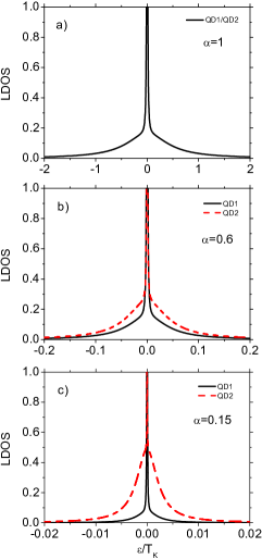
Figure 2: Local density of states for the quantum dots QD1 and QD2 obtained for indicated values of $\alpha$ and for $q=0.99$. Here, direct hopping between the dots is not allowed, because $t=0$.

In this section we consider the situation when dots are not directly coupled, which corresponds to the case with vanishing interdot tunnel coupling parameter $t=0$. On the other side, one should remember that dots are still coupled (indirectly) through the leads what is reflected in finite values of the off-diagonal coupling matrix elements, i.e., $q\neq 0$. In this situation bonding and antibonding levels, created due to indirect couplings, coincide. In Fig. 2 we show local density of states for QD1 and QD2 for large off-diagonal matrix couplings ($q=0.99$) and for different values of the asymmetry parameter $\alpha$. Firstly, it is clearly presented that the broad and narrow Kondo peaks in the LDOS are superimposed at energy $\varepsilon=0$ and the LDOS displays behavior typical for the Dicke effect. By analogy to the original Dicke phenomenon, one may associate the narrow (broad) central peak in LDOS with a subradiant (superradiant) state. The subradiant (superradiant) state corresponds to longlived (shortlived) state. For symmetric coupling $\alpha=1$ the LDOS for QD1 and QD2 are the same (see Fig. 2(a) but when asymmetry appears in couplings ($\alpha\neq 1$) this ceases to be true and the LDOS for both dots have different line shape. As $\alpha$ drops down the widths of the Kondo peaks for both dots also diminish. With decreasing $\alpha$ the broad part of the LDOS for the quantum dot strongly coupled to the leads (QD2) becomes more pronounced, whereas the narrow one becomes narrower. The two peaks corresponding to subradiant and superradiant state are well distinguishable. As a result, the Dicke effect in LDOS for QD2 is more distinct.

Figure 3: The transmission probability calculated for indicated values of $\alpha$ and for $q=0.99$ and for $t=0$. The transmission probability has well-defined Dicke line shape.

The Dicke effect is also noticed in the transmission shown in Fig. 3. This situation is analogous to that reported in the case of the spin Kondo effect in parallel double dot system. trochaJNN The Dicke peak appears in the transmission because the phases of the transmission amplitudes for bonding and antibonding channels are equal at zero energy. Thus, the two contributions adds constructively leading to the maximum transmission at $\varepsilon=0$. However, now there is no dip structure at zero energy for $q=1$ (originating from the complete destructive interference), which will be explained further. Moreover, the effect is preserved for various values of the asymmetry parameter $\alpha$. It is worth noting that the linear conductance (see Eq. (14)) reaches unitary limit (two quanta of $e^{2}/h$). When $\alpha$ is reduced the effective Kondo temperature also decreases what can be seen looking at the energy scale in Figure 2. The origin of this effect comes from the fact that when $\alpha$ decreases one of the dots becomes detached from the electrodes. Then, the rate of the higher order tunneling events (which leads to the Kondo anomaly-see explanation in the Introduction) also diminishes and finally for $\alpha=0$, when one of the dot is totally disconnected from the leads, there is no possibility for such events and no Kondo effect is expected.

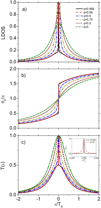
Figure 4: Local density of states for the both dots (a) Friedel phase (b) and the transmission (c) calculated for indicated values of the $q$ and for $\alpha=1$ and for $t=0$. The well-defined Dicke line shape is only preserved for indirect coupling parameter $q$ close to 1.

As we mentioned in Section II.1 the off-diagonal matrix elements $\Gamma^{\beta}_{12}$ may be significantly reduced, so it is desired to analyze this case. In Fig. (4) we plotted the LDOS, Friedel phase and the transmission for various values of the parameter $q$ which is directly related with amplitude of the off-diagonal matrix elements. The Friedel phase is related to the LDOS by the following equation: $d\theta_{F}/d\varepsilon=\pi D(\varepsilon)$ with $D(\varepsilon)$ being relevant density of states. One can notice that Dicke effect in LDOS can be found only when off-diagonal matrix elements are large, i.e., $q$ close to $1$. With decreasing $q$ the Dicke line shape is transformed in usual Lorenzian line. Similar behavior is observed in the transmission (see Fig. 4(c)). In inset of Fig. 4(c)) we show that the narrow part of the peak has also well defined shape as the broad one. Moreover, when $q$ is closer and closer to 1 then the narrow peak becomes more and more narrower. This is reflected in abrupt (but continuous as long as $q\neq 1$ ) change by $\pi$ of Friedel phase around $\varepsilon=0$ for $q$ close to $1$. It is also found that the Dicke effect also disappears in transmission when $q$ is maximal ($q=1$). When $q=1$ the transmission probability has Lorenzian shape and is described by formula,

$$T(\varepsilon)=\frac{1}{2}\left(\frac{(1+\alpha)^{2}\tilde{\Gamma}^{2}}{(1+\alpha)^{2}\tilde{\Gamma}^{2}+(\tilde{\varepsilon}_{0}-\varepsilon)^{2}}\right),$$ (15)

where $\tilde{\Gamma}=\tilde{b}^{2}\Gamma/2$. This equation clearly shows that no Dicke effect should be expected for $q=1$. This result resembles that obtained for a noninteracting system shahbazyan . However, in the Kondo regime the situation is much more complex. To show this, let us first consider the case with $q=1$ and symmetric couplings, $\alpha=1$. It is well known that for symmetric ($\alpha=1$) noninteracting ($U=0$) system as $q$ tends to $1$ one of the peaks becomes progressively narrowed and finally for $q=1$ a BIC emerges shahbazyan ; solisPLA . As a result the transmission reveals simple lorenzian lineshape. One may naively believe that similar situation occurs in the Kondo regime. However, this can not be true because when the indirect coupling strength is equal to the dot-lead coupling ($\Gamma_{12}=\Gamma_{11}=\Gamma_{22}$), the indirect tunneling processes completely destroy coherent higher-order tunelling events leading to complete suppression of the Kondo resonance. wen One can also look at this from the another point of view and explain this as follows: As the antibonding state becomes a BIC, it is totally decoupled from the leads and there is no possibility for an electron to exchange between the two molecular states. Thus, no Kondo effect appears as the corresponding Kondo temperature is equal to zero.

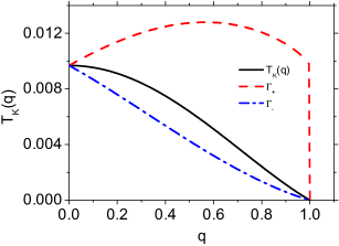
Figure 5: The Kondo temperature calculated as a function of parameter $q$ and renormalized width $\tilde{\Gamma}_{+}$ ($\tilde{\Gamma}_{-}$) coresponding to the bonding (antybonding) level calculated for $\alpha=1$ and for $t=0$.

To support these predictions we calculated the Kondo temperature for arbitrary value of the parameter $q$. The Kondo temperature for the symmetric case, $\alpha=1$, acquires the following form $T_{K}\equiv\sqrt{\tilde{\varepsilon}_{0}^{2}+\tilde{\Gamma}^{2}(1-q^{2})^{2}}$. In the deep Kondo regime the renormalized parameter $\tilde{\varepsilon}_{0}$ is equal to zero, which is shown in the Appendix, and thus the above formula clearly show vanishing of the corresponding Kondo temperature as $q$ tends to $1$. In Fig. 5 the Kondo temperature is displayed as a function of parameter $q$. For comparison we also plot the $q$ dependence of the renormalized widths of the bonding and antibonding levels, $\tilde{\Gamma}_{b}$ and $\tilde{\Gamma}_{a}^{2}$, respectively. In the case $q_{L}=q_{R}=q$, the widths acquire the following form $\tilde{\Gamma}_{b}=\tilde{b}^{2}\Gamma_{b}$, $\tilde{\Gamma}_{a}=\tilde{b}^{2}\Gamma_{a}$ with $\Gamma_{b,a}=\frac{1}{2}(\Gamma_{11}+\Gamma_{22})\pm q\sqrt{\Gamma_{11}\Gamma_{22}}$ and $\Gamma_{ii}=\Gamma_{ii}^{L}+\Gamma_{ii}^{R}$ for $i=1,2$. The characteristic widths for both distinct channels behave in different way with varying the strength of the off-diagonal tunneling processes. One can notice that the renormalized width for the bonding channel changes non-monotonically but rather slowly, whereas the one for the antibonding channel drops monotonically to zero as $q$ reaches maximum value. This behavior is consistent with the predictions given in Ref. lim, with one exception. The vanishing of $\tilde{\Gamma}_{a}^{2}$ when $q$ is maximal is responsible for the suppression of the Dicke effect. In contrast to Ref. lim, the width $\tilde{\Gamma}_{b}^{2}$ drops to zero for $q=1$ due to vanishing of the boson field. We also emphasize that for $q\in(0,1)$, the $\alpha$ dependances of the renormalized widths for both channels are different. For large values of the $q$ the width $\tilde{\Gamma}_{a}$ changes little with $\alpha$.

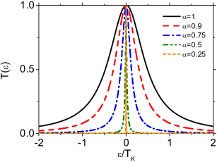
Figure 6: Graphical illustration of the Equation 16. The transmission probability calculated for indicated values of the $\alpha$ and for $q=0$.

However, the Kondo effect is also destroyed in more general case, i.e., for $q=1$ and arbitrary $\alpha$. This can be understood when one notice that transmission (15) depends on renormalized parameter $\tilde{b}$ which vanishes in this case. In the SBMF formalism this is manifested as lack of solutions of the self-consistent equations (9) and (10) (which then form a contradictory system of equations).

On the other side, for $q=0$ the following formula describes the transmission probability,

$$T(\varepsilon)=\frac{1}{2}\left[\frac{\tilde{\Gamma}^{2}}{\tilde{\Gamma}^{2}+(\tilde{\varepsilon}_{0}-\varepsilon)^{2}}+\frac{\alpha^{2}}{\alpha^{2}\tilde{\Gamma}^{2}+(\tilde{\varepsilon}_{0}-\varepsilon)^{2}}\right].$$ (16)

Figure 6 illustrates graphically Eq. (16) for indicated values of the asymmetry parameter $\alpha$. This plot clearly shows, as explained earlier, that the width of the Kondo peak decreases as $\alpha$ is reduced. This case resembles the spin Kondo effect in single-level quantum dot coupled to ferromagnetic leads martinekPRL03 . Then the asymmetry parameter $\alpha$ can be assigned with lead’s (pseudo)polarization in the following way $\tilde{p}=(1-\alpha)/(1+\alpha)$ trochaPRB10 . Increasing pseudopolarization (decreasing $\alpha$) the Kondo effect is suppressed which is in agreement with Refs. trochaPRB10, ; martinekPRL03, . In the presence of asymmetry in couplings ($\alpha<1$) the Kondo temperature should be defined by geometric mean as: $T_{K}\equiv\sqrt{\tilde{\Gamma}_{1}\tilde{\Gamma}_{2}}=\tilde{\Gamma}\sqrt{\alpha}$ (remembering that $\tilde{\varepsilon}_{0}\rightarrow 0$ in deep Kondo regime). Fig. 7 shows $\alpha$ dependence of the Kondo temperature for case of $q=0$.

Figure 7: The Kondo temperature calculated as a function of the asymmetry parameter $\alpha$ for $q=0$ and for $t=0$.

In the present case, $q=0$, electrons may travel only directly through dot QD1 or QD2 thus the reduction of the Kondo temperature with decreasing $\alpha$ clearly reflects the suppression of Kondo fluctuations in the DQD (due to reduction of the charge exchange between the dots) as one of the dot becomes detached from the leads and Kondo effect diminishes .

Similar dependance on parameter $q$ can be noticed in the differential conductance which is displayed in Fig. 8. The differential conductance is symmetric in respect to the zero bias point, thus we plot only its bias dependance for nonnegative bias voltage. For $q$ close to unity the differential conductance acquires Dicke line shape. At zero bias the differential conductance approaches unitary limit ($2e^{2}/h$) for all $q<1$. For $q$ close to $1$ the differential conductance drops very fast to the half of the zero bias value with increasing the bias voltage and next decreases slowly with further increasing of the bias voltage. Such a sudden drop of the differential conductance is absent for smaller values of the parameter $q$. This feature in the differential conductance is related to Dicke resonance.

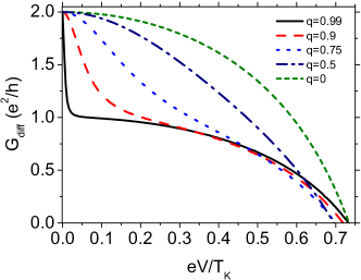
Figure 8: Differential conductance as a function of bias voltage calculated for indicated values of parameter $q$ ($q_{L}=q_{R}=q$) and for $\alpha=1$, $t=0$.

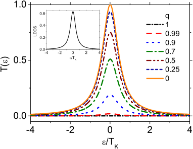
Figure 9: The transmission coefficient calculated for indicated values of the parameter $q$ ($q_{L}=-q_{R}=q$) and for $\alpha=1$. The inset show corresponding LDOS which is independent on the value of $q$.

As we mentioned in Sec. I the off–diagonal elements of the coupling matrix can have opposite signs. Specifically, we examine the case $q_{L}=q$ and $q_{R}=-q$. At the beginning we assume symmetric couplings, i.e., $\alpha=1$. Then for maximal value of the parameter $q$ ($q=1$) each DQD’s molecular state couples to different reservoirs and as there is no connection between them, the current doesn’t flow. This effect originates from the totally destructive quantum interference which leads to vanishing of the transmission even if the LDOS of each dots is finite. It is wort noting that both LDOS and the corresponding Kondo temperature do not depend on the parameter $q$, as the contributions from nondiagonal processes, refereing to the left $L$ and right $R$ lead, cancel each others. This implies that the presented effect originates fully from the quantum interference. One can notice that decreasing the value of the parameter $q$, the transmission can be recovered as is shown in Fig. 9. Finally, for $q=0$ the maximal value of the transmission is restored. This is because as the value of the off-diagonal matrix elements are decreased the destructive interference becomes totally suppressed, and thus, for zero value of the nondiagonal couplings the zero bias conductance is fully restored. This can be shown more formally by performing the transformation of the dots operators to the bonding-like ($d_{b}=1/\sqrt{2}(d_{1}+d_{2})$) and antibonding-like ($d_{a}=1/\sqrt{2}(d_{1}-d_{2})$) state. The corresponding couplings to the left lead acquires form $\tilde{\Gamma}_{b,a}^{L}=\frac{1}{2}(\tilde{\Gamma}_{11}^{L}+\tilde{\Gamma}_{22}^{L})\pm q\sqrt{\tilde{\Gamma}_{11}^{L}\tilde{\Gamma}_{22}^{L}}$, whereas couplings to the right electrode is given by $\tilde{\Gamma}_{b,a}^{R}=\frac{1}{2}(\tilde{\Gamma}_{11}^{R}+\tilde{\Gamma}_{22}^{R})\mp q\sqrt{\tilde{\Gamma}_{11}^{R}\tilde{\Gamma}_{22}^{R}}$. Now, it is clear that for $\alpha=1$ and $q=1$ the bonding state is coupled to (decoupled from) left (right) lead, whereas antibonding state is coupled to (decoupled from) right (left) electrode. As the parameter $q$ becomes less than $1$, the decoupled states from given leads for $q=1$ start to bound with them. As a result the transmission grows with decreasing the value of the parameter $q$.

Another interesting quantum interference effect can be found changing the asymmetry in couplings of two dots to the leads. At the beginning we keep $q$ equal to $1$ and change the parameter $\alpha$ in the interval $\langle 0,1\rangle$. As before the transmission becomes recovered as the asymmetry increases [see Fig. 10]. However, in comparison to the previous case, a new feature emerges in the transmission. More specifically, the dip structure appears in the vicinity of the zero energy. At $\varepsilon=0$ the transmission drops to zero which results in vanishing of the linear conductance. Thus, the zero bias Kondo anomaly is totally suppressed for any value of the asymmetry parameter $\alpha$. To verify this effect experimentally it is desired to measure the differential conductance as a function of bias voltage. In Fig. 11 we displayed bias voltage dependence of the differential conductance for indicated values of the asymmetry parameter $\alpha$. These results show that applying finite bias voltage, the differential conductance (which is zero at zero bias for all $\alpha$) is restored. The differential conductance becomes the most pronounced when one of the dot is almost decoupled from the leads, i.e., as $\alpha\rightarrow 0$, the differential conductance tend to unitary limit. However, with increasing asymmetry in the couplings (decreasing $\alpha$) the range of finite values of the differential conductance shrinks due to decreasing of the Kondo temperature. It is worth noting that the corresponding Friedel phase is a continuous function of energy – it does not suffer discontinuity at $\varepsilon=0$ because no BIC appears. However, the transmission at $\varepsilon=0$ vanishes, thus the phase of transmission amplitude should be discontinuous at $\varepsilon=0$.

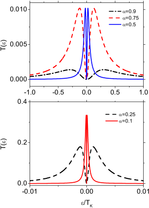
Figure 10: The transmission coefficient calculated for indicated values of the parameter $\alpha$ and for $q_{L}=-q_{R}=1$.

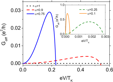
Figure 11: Differential conductance as a function of bias voltage calculated for indicated values of the parameter $\alpha$ and for $q_{L}=-q_{R}=1$, $t=0$.

III.2 Fano effect

Here, we show the results obtained for nonzero interdot hopping parameter ($t\neq 0$). In present situation the interdot hopping term lifts the degeneracy and the bonding and the antibonding levels are split away. As a result, the density of states of the DQD system coupled to the leads consists of two Kondo peaks; a broad peak centered at the bonding state and a narrow one corresponding to the antibonding state. This is clearly showed in Fig. 12(a)) where the LDOS for both dots is plotted for maximal off-diagonal matrix elements ($q=1$). It is very interesting that the narrow peaks in LDOS for QD1 and QD2 have opposite symmetries. The LDOS for QD1 reaches zero for negative energy, whereas the one for QD2 comes to zero for positive energy. Usually, when the asymmetry in coupling of two dots to the leads is reduced the width of bonding (antibonding) state increases (decreases). Finally, for $\alpha=1$ (full symmetric system) the antibonding states is decoupled from the leads and acquires $\delta$-Dirac shape (it becomes a BIC), whereas the bonding state acquires the width of $2\tilde{\Gamma}$. On the other side, when the asymmetry in coupling of two dots to the leads is increased then the width of bonding (antibonding) state decreases (increases) and for $\alpha=0$ the two resonances acquire the same width. However, in current problem the situation is more complex because the level’s widths are renormalized by factor $\tilde{b}^{2}$ which has to be obtained self-consistently for each $\alpha$. Now it is only true that relative width of the bonding state to the width of the antibonding state grows as $\alpha$ increases, and are the same for $\alpha=0$. However, due to widths renormalization both peaks in LDOS may have smaller widths for small $\alpha$ with comparison to the width of the narrow peak for large $\alpha$ (but not $\alpha\approx 1$) (for instance for $\alpha=0.15$ both resonances are merged into narrow resonance for $\alpha=0.8$). Similar behavior is observed in the LDOS for dots QD1 and QD2. Another feature is that for smaller values of the $\alpha$ only LDOS for QD2 may reach zero value at some energy.

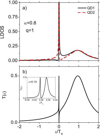
Figure 12: Local density of states for the both dots (a) and the transmission probability (b) calculated for $q=1$, $\alpha=0.8$ and for $t=0.8$. The existence of the Fano-Kondo effect is well visible. The inset shows the transmission probability obtained for $q=1$ and for $\alpha=0.15$.

Figure 13: The transmission probability calculated for $\alpha=0.8$, $t=0.8$, and for $q=0.99$. Even a small shift in $q$ leads to the considerably changes in the transmission probability within the antibonding level considerably (compare with Fig. 12).

The above behavior of LDOS for $\alpha\in(0,1)$ results in Fano antiresonance in the transmission probability. The corresponding transmission probability calculated for $q=1$ and $\alpha=0.8$ is displayed in Fig. 12(b). One can notice that the transmission reveals the antiresonance character with a characteristic Fano line shape. In turn, the transmission function corresponding to the bonding state is relatively broad and (roughly) Lorenzian. In inset of Fig. 12(b) the $T(\varepsilon)$ is plotted for greater asymmetry in coupling of two dots to the leads ($\alpha=0.15$). It is noticed that the antiresonance behavior is still preserved but now the widths’ ratio of the narrow resonance with respect to the broad one is much larger in comparison to the previous case (i.e., when $\alpha=0.8$). With decreasing $\alpha$ the widths of both peaks also decrease which can be seen looking at the energy scales for both cases. This means that the Kondo temperature is also lowered as $\alpha$ decreases (as was shown in the previous section). For $q=1$ the transmission probability has poles at,

$$\varepsilon=\tilde{\varepsilon}_{0}-\frac{2\sqrt{\alpha}}{1+\alpha}\tilde{t}.$$ (17)

It is worth to mention that at this energy the phase of the transmission amplitude suffers discontinuity. This is no more true for $q<1$, because then the transmission probability has complex poles. In turn, for $q<1$ the transmission probability does not reach zero and for specific value of $q$ antiresonance behavior is less visible. Even a small shift in $q$ change the transmission probability within the antibonding level considerably, which is showed in Fig. 13.

At this point we should remark that the slave boson mean field approach does not take into account the level renormalization arising due to coupling of dots to the leads. Such a renormalization should lead to splitting of the zero bias anomaly for specific cases. trochaPRB10 The level splitting can occurs due to asymmetry in coupling of the dots to the leads, i.e., for $\alpha<1$ as has been shown in Ref. trochaPRB10, by means of the scaling technique. However, such a splitting can also be induced by indirect coupling of the dots. One can show that the splitting is proportional to the strength of the indirect coupling. Moreover, the level renormalization of a given state is proportional to the coupling strength of the other level. This implies that for $q$ close to $1$ the bonding-like level will be only weakly renormalized, whereas the antibonding-like level will experience strong renormalization.

Thus, the transmission described in Sec. III.1 should resembles that from Fig. 13 but with the broad peak pinned close to $\varepsilon=0$ and the narrow maximum shifted up in energy for relatively large value of parameter $q$. One can show this more formally including corrections in molecular-like levels due to mentioned renormalization.

To correct the drawback of the SBMF method one can by hand introduce the mentioned renormalization of the levels as follows: $\varepsilon_{b}=\varepsilon_{0}+\delta\varepsilon_{b}$ and $\varepsilon_{a}=\varepsilon_{0}+\delta\varepsilon_{a}$ (with $t=0$ for the sake of simplicity). Here, $\delta\varepsilon_{i}$ are the corrections due to indirect coupling of the dots levels. These corrections should be determined using relevant technique, as for instance earlier mentioned scaling procedure. However, as the SBMF technique fails for nondegenerate states, one can not introduce by hand the renormalized levels into self-consistent equations of the form (9) and (10) derived within bonding and antibonding states basis. Thus, we give here only rough estimation and some predictions implying from the levels scaling. Such approach should deliver qualitatively good insight into Kondo peak splitting phenomenon, however to obtain quantitatively consistent results more reliable technique should be applied for the considered problem. For the sake of simplicity we analyze only the symmetric case ($\alpha=1$). Introducing the level renormalization the transmission acquires the following form:

$$T(\varepsilon)=\frac{\tilde{\Gamma}^{2}(1-q)^{2}}{(\varepsilon-\tilde{\varepsilon}_{a})^{2}+\tilde{\Gamma}^{2}(1-q)^{2}}+\frac{\tilde{\Gamma}^{2}(1+q)^{2}}{(\varepsilon-\tilde{\varepsilon}_{b})^{2}+\tilde{\Gamma}^{2}(1+q)^{2}}$$ (18)

with renormalized bonding ($b$) and antibonding ($a$) levels of the following assumed form trochaUnpub :

$$\varepsilon_{i}=\varepsilon_{0}+\Gamma_{\bar{i}}\Delta$$ (19)

Here, $\Delta$ trochaApp stands for some function which in general depends on the system’s parameters (like bandwidth, dots energy levels, couplings). For the sake of simplicity we assume $\Delta$ to be a constant number and being maximum value of function $\Delta(q)$ obtained from the scaling procedure, i.e. when $q=1$. Equation (18) clearly shows that Kondo peak becomes split due to the level renormalization originating from indirect tunneling between the dots. In Fig. 14 we display expected lineshape in the transmission for relatively large value of parameter $q$. The splitting in the transmission should decrease with decreasing the value of parameter $q$ and beyond a certain value of $q$ the splitting ceases to be visible. For $q=0$ (and $\alpha=1$) no splitting occurs.

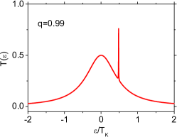
Figure 14: The transmission coefficient including the level renormalization calculated for $\alpha=1$ and for $q_{L}=q_{R}=0.99$.

IV Summary and conclusions

In this paper we have investigated electronic properties of double quantum dots coupled to external leads. The dots have been coupled both via hopping term and Coulomb interaction. Moreover, we have considered also the effects of indirect tunneling between the dots through the leads. Employing the slave-boson mean field approach the local density of states for both dots, the Friedel phase and the transmission in Kondo regime have been calculated. Moreover, to be more familiar with experiment we have calculated the corresponding differential conductance.

We have shown that for some set of parameters the Dicke-and Fano-like resonances may appear in the considered system. More specifically, it has been noticed that for zero interdot hopping parameter $t$ the LDOS of each QD consist of broad and narrow Kondo peaks that are superimposed. As in original Dicke effect one may associate narrow (broad) central peak in LDOS with a subradiant (superradiant) mode. Moreover, Dicke line shape has been found in the transmission and in the differential conductance. We have observed that this effect is very sensitive to the strength of the off-diagonal matrix elements; with reducing the value of the off-diagonal matrix elements the Dicke line both in LDOS and the transmission is transformed into usual Lorenzian line. It has been found that when the interdot tunneling is allowed the transmission probability may reveal the antiresonance behavior with a characteristic Fano line shape. Moreover, we have noticed that the line shape of the antiresonance is also very susceptible to the change of the value of the off-diagonal matrix elements.

We have also calculated the Kondo temperature, and also have shown that the latter becomes suppressed with increasing asymmetry in the dot-lead couplings when there is no indirect coupling. Moreover, when the indirect coupling is turned on, the characteristic widths for both distinct channels behave in different way with varying strength of the off-diagonal tunneling processes. We found also that the corresponding Kondo temperature is totally suppressed for maximal value of the indirect coupling and no Kondo effect occurs. Moreover, we have also included level renormalization effects due to indirect coupling phenomenon, which leads to the splitting of the Kondo peak.

Appendix A Proof of $\tilde{\varepsilon}_{0}\rightarrow 0$ in deep Kondo regime

Here, we show that in deep Kondo regime the renormalized parameter $\tilde{\varepsilon}_{0}$ is equal to zero and, thus, the Kondo temperature strictly correspond to to the renormalized width $\tilde{\Gamma}$ of the Abricolov-Suhl resonance. This can be shown analytically by integrating self-consistent equations for slave-boson parameters, $\tilde{b}$, $\lambda$, written in representation of bonding and antibonding states.

In the basis of the bonding and antibonding states the Hamiltonian of the system becomes diagonal for $\varepsilon_{1}=\varepsilon_{2}\equiv\varepsilon_{0}$ and acquires the following form:

$$\hat{H}=\hat{H}_{c} + \sum_{i=b,a}\limits\varepsilon_{i}d^{\dagger}_{i}d_{i}+Un_{b}n_{a}$$ (20)

$$+ \sum_{\mathbf{k}\beta}\limits\sum_{i=e,o}\limits(V_{i\mathbf{k}}^{\beta}c^{\dagger}_{\mathbf{k}\beta}d_{i}+\rm H.c.),$$

with $\varepsilon_{b}=\varepsilon_{0}+t$, $\varepsilon_{a}=\varepsilon_{0}-t$. In further considerations we assume $t=0$, thus, $\varepsilon_{b}=\varepsilon_{a}=\varepsilon_{0}$.

In the mean field slave boson representation the Hamiltonian (20) acquires the following form:

$$\tilde{H}^{MF}=\hat{H}_{c} + \sum_{i=\emph{b,a}}\limits\tilde{\varepsilon}_{0}f^{\dagger}_{i}f_{i}+\lambda\left(\tilde{b}^{2}-1\right)$$ (21)

$$+ \sum_{{\mathbf{k}}\beta}\sum_{i=\emph{b,a}}\limits(\tilde{V}_{i\mathbf{k}}^{\beta}c^{\dagger}_{{\mathbf{k}}\beta}f_{i}+{\rm H.c.}).$$

The self-consistent equations determining the unknown parameters $\tilde{b}$ and $\lambda$ have the form of Eqs. (9) and (10) with lesser Green’s function $\langle\langle f_{i}|f^{{\dagger}}_{j}\rangle\rangle^{<}_{\varepsilon}$ defined in the basis of the bonding and antibonding states. The lesser bonding and antibonding Green’s function has the following form:

$$G_{ii}^{<}(\varepsilon)=\frac{f(\varepsilon)\tilde{\Gamma}_{i}}{(\varepsilon-\tilde{\varepsilon}_{0})^{2}+(\tilde{\Gamma}_{i}/2)^{2}}.$$ (22)

At $T=0$ K $f(x)=\theta(-x)$ and the integration of the self-consistent equations is straightforward integrand leading to the following expressions:

$$\frac{1}{\pi}\sum_{i=b,a}\limits{\rm Im}\left[\ln\left(\frac{\varepsilon_{0}+i\tilde{\Gamma}_{i}/2}{D}\right)\right]=1-\tilde{b}^{2},$$

$$\frac{1}{2\pi}\sum_{i=b,a}\limits\tilde{\Gamma}_{i}{\rm Re}\left[\ln\left(\frac{\varepsilon_{0}+i\tilde{\Gamma}_{i}/2}{D}\right)\right]+\lambda\tilde{b}^{2}=0.$$ (23)

In the deep Kondo regime we can approximate: $1-\tilde{b}^{2}\approx 1$ and $\lambda\approx-\varepsilon_{0}$ and then Eqs. (A) simplify to the following equations:

$$\sum_{i=b,a}\limits{\rm Im}\left[\ln\left(\frac{\varepsilon_{0}+i\tilde{\Gamma}_{i}/2}{D}\right)\right]=\pi,$$

$$\sum_{i=b,a}\limits\Gamma_{i}{\rm Re}\left[\ln\left(\frac{\varepsilon_{0}+i\tilde{\Gamma}_{i}/2}{D}\right)\right]=2\pi\varepsilon_{0}.$$ (24)

Here, we consider only the symmetric case, $\alpha=1$, however, extension to arbitrary $\alpha$ is straightforward. For $\alpha=1$ and $q_{L}=q_{R}=q$, the couplings to the bonding and antibonding states acquires the following form, $\Gamma_{b,a}=(1\pm q)\Gamma$. Combining two equations (A) one arrives with equation:

$$(\tilde{\varepsilon}_{0}+i\tilde{\Gamma}_{b}/2)(\tilde{\varepsilon}_{0}+i\tilde{\Gamma}_{a}/2)\left(\frac{\tilde{\varepsilon}_{0}+(\tilde{\Gamma}_{b}/2)^{2}}{\tilde{\varepsilon}_{0}+(\tilde{\Gamma}_{a}/2)^{2}}\right)^{\frac{q}{2}}=D^{2}\exp\left[\left(\frac{i}{2}+\frac{\varepsilon_{0}}{\Gamma}\right)2\pi\right],$$ (25)

which real and imaginary parts satisfy the following equalities:

$$\left(\tilde{\varepsilon}_{0}^{2}+\frac{1}{4}\tilde{\Gamma}_{b}\tilde{\Gamma}_{a}\right)\left(\frac{\tilde{\varepsilon}_{0}+(\frac{\tilde{\Gamma}_{b}}{2})^{2}}{\tilde{\varepsilon}_{0}+(\frac{\tilde{\Gamma}_{a}}{2})^{2}}\right)^{\frac{q}{2}} = -D^{2}\exp\left(\frac{2\pi\varepsilon_{0}}{\Gamma}\right),$$ (26)

$$\tilde{\varepsilon}_{0}(\tilde{\Gamma}_{b}+\tilde{\Gamma}_{a})\left(\frac{\tilde{\varepsilon}_{0}+(\frac{\tilde{\Gamma}_{b}}{2})^{2}}{\tilde{\varepsilon}_{0}+(\frac{\tilde{\Gamma}_{a}}{2})^{2}}\right)^{\frac{q}{2}} = 0.$$ (27)

Equation (27) is satisfied if $\tilde{\varepsilon}_{0}=0$ or $\tilde{b}^{2}=0$. However, the later solution leads to nonphysical value for $\tilde{\varepsilon}_{0}$, thus, the only solution must be $\tilde{\varepsilon}_{0}=0$. This result clearly shows that in deep Kondo regime slave-boson parameter $\tilde{\varepsilon}_{0}$ vanishes, Q.E.D.

Introducing the solution for $\tilde{\varepsilon}_{0}$ into Eq. (26) one finds,

$$\tilde{b}^{2}=\frac{2D}{\Gamma}\frac{(1-q)^{\frac{q-1}{2}}}{(1+q)^{\frac{q+1}{2}}}\exp\left(\frac{\pi\varepsilon_{0}}{\Gamma}\right).$$ (28)

It is worth noting that the above equation does not determine the value of $\tilde{b}^{2}$ for $q=1$ when the SBMF method fails.

References

- (1) J. Kondo, Prog. Theor. Phys. 32, 37 (1964).
- (2) S. M. Cronenwett, T. H. Oosterkamp and L. P. Kouwenhoven, Science 281, 540 (1998); S. Sasaki,S. De Franceschi, J. M. Elzerman, W. G. van der Wiel, M. Eto, S. Tarucha and L. P. Kouvenhoven, Nature (London) 405, 764 (2000).
- (3) D. Goldhaber-Gordon, H. Shtrikman, D. Mahalu, D. Abusch-Magder, U. Meirav and M. A. Kastner, Nature (London) 391, 156 (1998).
- (4) L. I. Glazman and M. E. Raikh JETP Lett. 47, 452 (1988); T. K. Ng and P. A. Lee, Phys. Rev. Lett. 61, 1768 (1988).
- (5) G. Grüner and A. Zawadowski, Rep. Prog. Phys. 37, 1497 (1974); G. Zaránd and A. Zawadowski, Phys. Rev. Lett. 72, 542 (1994).
- (6) D. Boese, W. Hofstetter, and H. Schoeller, Phys. Rev. B 64, 125309 (2001).
- (7) P. G. Silvestrov and Y. Imry, Phys. Rev. B 75, 115335 (2007).
- (8) U. Wilhelm, J. Schmid, J. Weis and K. von Klitzing, Physica E 14, 385 (2002).
- (9) A. Hübel, K. Held, J. Weis and K. von Klitzing, Phys. Rev. Lett. 101, 186804 (2008).
- (10) Q.-F. Sun and H. Guo, Phys. Rev. B 66, 155308 (2002).
- (11) D. Sztenkiel, R. Świrkowicz, J. Phys.: Condens. Matter 19, 256205 (2007).
- (12) D. Sztenkiel, R. Świrkowicz, J. Phys.: Condens. Matter 19, 386224 (2007).
- (13) A. W. Holleitner, A. Chudnovskiy, D. Pfannkuche, K. Eberl, and R. H. Blick, Phys. Rev. B 70, 075204 (2004).
- (14) S. Lipiński and D. Krychowski, Phys. Status Solidi b 243, 206 (2005).
- (15) T. Pohjola, H. Schoeller and G. Schön, Europhys. Lett., 54, 241 (2001).
- (16) E. Vernek, N. Sandler, S.E. Ulloa, E.V. Anda, Physica E, 34, 608 (2006).
- (17) M. Sindel, A. Silva, Y. Oreg, and J. von Delft, Phys. Rev. B 72, 125316 (2005).
- (18) R. López, D. S nchez, M. Lee, M.-S. Choi, P. Simon, K. Le Hur, Phys. Rev. B 71, 115312 (2005).
- (19) R. M. Konik, Phys. Rev. Lett 99, 076602 (2007).
- (20) G.-M. Zhang, R. Lü,2 Z.-R. Liu, and L. Yu, Phys. Rev. B 72, 073308 (2005).
- (21) G.-H. Ding, C. K. Kim, K. Nahm, Phys. Rev. B 71, 205313 (2005).
- (22) Y. Tanaka, N. Kawakami, Phys. Rev. B 72, 085304 (2005).
- (23) J. Wen, J. Peng, B. Wang, and D. Y. Xing, Phys. Rev. B 75, 155327 (2007).
- (24) T. Kubo, Y. Tokura, and S. Tarucha, Phys. Rev. B 77, 041305(R) (2008).
- (25) J. von Neumann, E. Wigner, Phys. Z. 30, 465 (1929); L. Fonda, R.G. Newton, Ann. Phys. 10, 490 (1960) ; F.H. Stillinger, D.R. Herrick, Phys. Rev. A 11, 446 (1975).
- (26) T. Kubo, Y. Tokura, and S. Tarucha, Phys. Rev. B 83, 115310 (2011).
- (27) S. A. Gurvitz, IEEE Trans. Nanotechnol. 4, 45 (2005).
- (28) T. Hatano, T. Kubo, Y. Tokura, S. Amaha, S. Teraoka, and S. Tarucha, Phys. Rev. Lett. 106, 076801 (2011).
- (29) V. Meden and F. Marquardt, Phys. Rev. Lett. 96, 146801 (2006).
- (30) V. Kashcheyevs, C. Karrasch, T. Hecht, A. Weichselbaum, V. Meden, and A. Schiller, Phys. Rev. Lett. 102, 136805 (2009).
- (31) R. H. Dicke, Phys. Rev. 89, 472 (1953).
- (32) R. H. Dicke, Phys. Rev. 93, 99 (1954).
- (33) U. Fano, Phys. Rev. 124, 1866 (1961).
- (34) T. V. Shahbazyan and M. E. Raikh, Phys. Rev. B 49, 17123 (1994).
- (35) P. A. Orellana, M. L. Ladrón de Guevara, and F. Claro, Phys. Rev. B 70, 233315 (2004).
- (36) T. Brandes, Phys. Rep. 408, 315 (2005).
- (37) P. Trocha, J. Barnaś, J. Phys.: Condens. Matter 20, 125220 (2008).
- (38) P. Trocha, J. Barnaś, Phys. Rev. B 78, 075424 (2008).
- (39) P. Trocha and J. Barnaś, J. Nanosci. Nanotechnol. 10, 2489 (2010).
- (40) B. Wunsch and A. Chudnovsky, Phys. Rev. B 68, 245317 (2003).
- (41) J. Göres, D. Goldhaber-Gordon, S. Heemeyer, M.A. Kastner, H. Shtrikman, D. Mahalu, and U. Meirav, Phys. Rev. B 62, 2188 (2000).
- (42) A. A. Clerk, X. Waintal, P. W. Brouwer, Phys. Rev. Lett. 86, 4636 (2001).
- (43) K. Kobayashi, H. Aikawa, S. Katsumoto, and Y. Iye, Phys. Rev. Lett. 88, 256806 (2002).
- (44) A. C. Johnson, C.M. Marcus, M. P. Hanson, and A.C. Gossard, Phys. Rev. Lett. 93, 106803 (2004).
- (45) S. Sasaki, H. Tamura, T. Akazaki, and T. Fujisawa, Phys. Rev. Lett. 103, 266806 (2009).
- (46) B. Bułka and P. Stefański, Phys. Rev. Lett. 86, 5128 (2001).
- (47) M. L. Guevara, F. Claro, P. A. Orellana, Phys. Rev. B 67, 195335 (2003).
- (48) H. Lu, R. Lü, and B.-F. Zhu, Phys. Rev. B 71, 235320 (2005).
- (49) F. Chi, J.-L. Liu, L.-L. Sun, J. Appl. Phys. 101, 093704 (2007).
- (50) P. Trocha, J. Barnaś, Phys. Rev. B 76, 165432 (2007).
- (51) R, Žitko, Phys. Rev. B 81, 115316 (2010).
- (52) T. Kubo, Y. Tokura, and S. Tarucha, Phys. Rev. B 74, 205310 (2006).
- (53) P. Coleman, Phys. Rev. B 29, 3036 (1984).
- (54) B. Solis, M.L. Ladrón de Guevara, P.A. Orellana, Phys. Lett. A 372, 4736 (2008).
- (55) J. S. Lim, M.-S. Choi, R. López, R. Aguado, Phys. Rev. B 74, 205119 (2006).
- (56) P. Trocha, Phys. Rev. B 82, 125323 (2010).
- (57) J. Martinek, Y. Utsumi, H. Imamura, J. Barnaś, S. Maekawa, J. König, and G. Schön, Phys. Lett. 91,127203 (2003); D. Matsubayashi and M. Eto, Phys. Rev B 75, 165319 (2007).
- (58) P. Trocha, (unpublished).
- (59) Within the scaling approach for the spinless Anderson model acquires the following form, with denoting a half-bandwidth at the end of scaling procedure.
- (60) At finite temperature the integrands appearing in the self-consistent equations can be evaluated analitically by means of contour integration. To satisfy Jordan’s lemma the integrand appearing in the equation of form (10) must be calculated with the help of lorenzian cut-off function, . Then, the results can be expressed by means of digamma function and Fermi-Dirac function, which for converge to the expressions derived in the Appendix.