The Entanglement of a Quantum Field with a Dispersive Medium

Abstract

In this Letter we study the entanglement of a quantum radiation field interacting with a dielectric medium. In particular, we describe the quantum mixed state of a field interacting with a dielectric through plasma and Drude models, and show that these generate very different entanglement behavior, as manifested in the entanglement entropy of the field. We also present a formula for a “Casimir” entanglement entropy, i.e. the distance dependence of the field entropy. Finally, we study a toy model of the interaction between two plates. In this model, the field entanglement entropy is divergent, however, as in the Casimir effect, its distance-dependent part is finite and the field matter entanglement is reduced when the objects are far.

The theory describing electromagnetic fluctuations in a linear material medium is an essential tool in understanding matter-radiation interaction. Classically, thermally excited fluctuations as well as purely quantum, zero temperature, fluctuations in macroscopic media have been widely studied in terms of susceptibilities (see e.g. Lifshitz and Pitaevskii (1984); Levin and Rytov (1967)). While the use of such response functions have been highly successful in describing various phenomena, the actual quantum state of the field is usually not described. Indeed, even at zero temperature, a field interacting with realistic materials (as opposed to idealized Dirichlet or Neumann boundaries), is in general not in a pure state and should be described in terms of a mixed state density matrix. In modern terms, this mixed state is viewed as a consequence of matter-field entanglement, and carries a nonvanishing von-Neuman entropy, sometimes called “entanglement entropy” (EE).

In this Letter we describe the quantum state associated with a field in a medium given a dielectric function $\varepsilon$. The effective action for such a field includes frequency dependence. Usually, such frequency dependent action is associated with response functions, however, here, we have to understand the action as specifying an instantaneous form for the photonic density matrix. We do this by describing the effective density matrix of the field.

As a measure of the field-matter entanglement, we use the entanglement entropy (EE) of the field. EE has been the subject of intense investigations in recent years, in a large variety of quantum systems, with applications to quantum information, condensed matter theory and high energy theory (For a review see e.g. Amico et al. (2008)). In particular, the entropy of radiation coupled to matter has been considered in numerous works. Usually the focus is on a single degree of freedom coupled to a bath of oscillators: For example, the entropy of a spin in the spin-boson model within the frame work of the Caldeira-Legget model Caldeira and Leggett (1981) was considered in Le Hur (2008) while the entanglement of a single radiation mode with an array of spins was studied in Lambert et al. (2004) for the Dicke model . On a different note, the EE of spatially separated intervals of vacuum (or ground state of a spin chains) has been considered in Marcovitch et al. (2009); Calabrese et al. (2009). Here we consider a situation distinct from these works, and more akin to the scenario considered in studies of Casimir and Van der Waals interactions between macroscopic bodies: that of a field in contact with macroscopic dispersive bodies.

Consider the electromagnetic field interacting with a dielectric medium at zero temperature. We assume that no external charges or currents are present and work in the gauge $A_{0}=0$. The long wave-length effective action,

$$S={1\over 4\pi}\int{\rm d}^{3}x{{\rm d}\omega}{\bf A}_{\omega}^{*}({\bf x})[{\omega}^{2}\varepsilon({\omega},{\bf x})-\nabla\times\nabla]{\bf A}_{\omega}({\bf x}),\,$$ (1)

encodes the field interaction with the material through the dielectric response function $\varepsilon({\omega},{\bf x})$. As we show below, the appearance of frequency dispersion in $\varepsilon({\omega},{\bf x})$ means that an action like (1) does not describe the state of the field as a ground state of a field Hamiltonian; indeed, the action is nonlocal in time and so cannot be quantized to yield a proper quantum Hamiltonian.

Clearly, one possible effect of coupling to the environment may be thermalization of our field. It is therefore tempting to try and describe the instantaneous state of such a field as effectively thermal i.e. $\rho\sim Z^{{-1}}e^{-\beta H_{eff}}$ for a reasonable effective field Hamiltonian $H_{eff}$. Such effective “Entanglement Hamiltonians” have been the focus on recent studies due to their relation to the conformal edge spectra of fractional quantum hall systems Li and Haldane (2008); Qi et al. (2011).

We show, however, that in the field-matter system, the field cannot be viewed as simply thermal. Rather, different ranges of momenta feel different effective temperatures. While the occupation probability of UV photons vanishes with high momenta, we still find that the field in (1) carries a logarithmic UV divergent quantum “zero point” entropy and show it’s cutoff dependence in (12).

Finally, we consider, a la Casimir, the distance dependence of the entropy associated with field interaction with a pair of objects separated by vacuum, and show a toy model in which the “Casimir” entanglement entropy is UV finite and decays with distance. Physically, this means that the field becomes more entangled with the plates as they come closer.

Here we study a simplified scalar field version of the electromagnetic field action (1).

$$S={1\over 4\pi}\int{\rm d}^{3}x{{\rm d}\omega}\phi_{\omega}^{*}({\bf x})[{\omega}^{2}\varepsilon({\omega},{\bf x})-\nabla^{2}]\phi_{\omega}({\bf x}).$$ (2)

Note that the UV dependence study bellow is valid for the full electromagnetic problem, since in homogenous systems (1) separates naturally into two scalar fields describing the two polarization modes. When the permittivity is independent of $\omega$, the action is local in time, and one can easily quantize the associated scalar action assuming the conjugate momentum $\pi_{\phi}$ can be expressed in terms of $\dot{\phi}$ and doesn’t depend on external fields. Such an action follows from the Hamiltonian $H={1\over 4\pi}\int{\rm d}^{3}x[{\pi^{2}\over\varepsilon({\bf x})}+(\nabla\phi)^{2}]$. It describes, at zero temperature, a pure state, and as such will have no entropy .

The situation is fundamentally different if $\varepsilon$ is $\omega$ dependent. The non-locality of the action (2) in time signals that our system is coupled to external degrees of freedom which have been integrated out, yielding a non trivial temporal response kernel. In such a case, the system cannot be in a pure state implying that our radiative system is entangled with the matter fields.

To proceed, let us briefly review the method of calculating entropies of Gaussian states (For details see, e.g. Botero and Reznik (2003); Plenio and Virmani (2007)). The calculation is facilitated by the fact that all information lies in the two point functions of the field. For a scalar field with $n$ degrees of freedom $\phi_{n}$ and conjugate momenta $\pi_{n}$, one defines the vector: $(O_{1},..O_{2n})=(\phi_{1},\pi_{1},..\phi_{n},\pi_{n})$. The state of the field is then determined by the covariance matrix:

$$\gamma_{jk}=2Re\langle(O_{j}-\langle O_{j}\rangle)(O_{k}-\langle O_{k}\rangle)\rangle.$$ (3)

$\gamma$ can be brought into a Williamson normal form $W\gamma W^{T}=diag(\mu_{1},...\mu_{n},\mu_{1},...\mu_{n})$ by means of a symplectic transformation $W\in Sp(2n)$ preserving the canonical commutation relations $[O_{j},O_{k}]=i\sigma_{j,k}$, where $\sigma$ is the $2n\times 2n$ matrix

$$\sigma=\oplus_{j=1}^{n}\left(\begin{array}[]{cc}0&1\\ -1&0\end{array}\right)~{}~{}~{}~{};~{}~{}~{}~{}W^{t}\sigma W=\sigma.$$

The occupation probability of the normal modes are directly related to the symplectic eigenvalues $\mu_{i}$ of $\gamma$. Finally, the density matrix can be written as:

$$\rho=Z^{-1}e^{-\sum_{i}u_{i}\Phi^{+}_{i}\Phi_{i}}~{};~{}u_{i}=\log{\mu_{i}+{1}\over\mu_{i}-{1}}$$ (4)

where $\Phi^{+}_{i}$ is a bosonic creation operators for the normal mode $i$. The entropy is given by:

$${\cal S}=\sum_{i}h(\mu_{i})~{};~{}h(\mu)={\mu+1\over 2}\log{\mu+1\over 2}-{\mu-1\over 2}\log{\mu-1\over 2}$$ (5)

An additional, technical simplification occurs, if we assume that no $\langle\phi\pi\rangle$ correlations are present. It is then known that the symplectic eigenvalues are square roots of eigenvalues of $\Gamma={\cal G}{\cal H}$, where ${\cal G}$ and ${\cal H}$ are field and field momentum two point functions, respectively.

For the translationally invariant medium the symplectic eigenvalues can be labeled by momentum and given by $\mu_{k}=2\pi^{-1}(g_{{\bf k}}h_{\bf k})^{{1/2}}$, where $g_{{\bf k}}h_{\bf k}$ is the product ${\cal G}{\cal H}$ in ${\bf k}$ space given by $g_{k}=\langle\phi^{2}\rangle_{\bf k}=\int{\rm d}{\bf x}e^{{i\bf x\cdot\bf k}}\langle\phi({\bf x},t^{\prime})\phi({\bf 0},t)\rangle|_{t^{\prime}\rightarrow t_{+}}$ and similarly $h_{k}=\langle\pi^{2}\rangle_{\bf k}$. The field entropy per unit volume can be written as:

$${{\cal S}_{field}}=-{V}^{-1}{\rm Tr}\rho_{field}\log\rho_{field}=\int{\rm d}{\bf k}h(\mu_{\bf k})$$ (6)

For concreteness, let us choose a typical dielectric function $\varepsilon$ to use in (7) and (8). We take: $\varepsilon({\omega},{\bf x})=1+4\pi\chi(\omega,{\bf x})$. With a typical susceptibiliy of the form $\chi_{b}={{\omega_{p}^{2}}\over(\omega_{0}^{2}-\omega^{2}-i\gamma_{p}\omega)}$ (for a conductor we will add a Drude function $\chi_{c}=\chi_{b}+i{\omega_{c}^{2}\over\omega(\gamma_{c}-i\omega)}$). The action (2) allows us to compute, per $k$ mode:

$$g_{k}=\int_{0}^{\infty}{\rm d}\omega{1\over{\omega^{2}\varepsilon({\bf k},i\omega)+k^{2}}}$$ (7)

and, using time point splitting,

$$h_{k}=\int_{0}^{\infty}{\rm d}\omega{1\over{\omega^{2}\varepsilon({\bf k},i\omega)+k^{2}}}(k^{2}+4\pi\omega^{2}\chi(i|\omega|)).$$ (8)

Using, the integrals (7),(8) and (4) we represent the density matrix as $\rho\sim exp(-\sum_{\bf k}u_{{\bf k}}\Phi^{+}_{{\bf k}}\Phi_{{\bf k}})$.

One may try to interpret this state as thermal, i.e.: $\rho\sim exp(-\beta H_{eff})$. The effective field Hamiltonian is then given by: $H_{eff}=\int{\rm d}{\bf x}{\rm d}{\bf x}^{\prime}\hat{u}({\bf x}-{\bf x}^{\prime})\Phi^{+}_{{\bf x}}\Phi_{{\bf x}^{\prime}}$ where $\hat{u}=\beta^{-1}\int{\rm d}{\bf k}u_{\bf k}e^{i{\bf k}\cdot({\bf x}-{\bf x}^{\prime})}$. However, we find that generically the fourier transformed $\hat{u}$ gives us a non-local $H_{eff}$.

Alternatively, we may interpret $u_{\bf k}$ as $u_{\bf k}=\beta_{k}E_{k,free}$ where $E_{k,free}$ are the photon energies without the interaction. Thus, different momenta ${\bf k}$ feel different effective temperatures. Estimating $u_{\bf k}$ from the integrals (7),(8), we find for the soft modes, $u_{\bf k}=\beta_{k}E_{k,free}\propto\sqrt{k}$ and so the effective temperature:

$$T_{k}\equiv{k\over\beta_{k}}\propto{\sqrt{k}}~{}~{}~{}as~{}~{}~{}~{}k\rightarrow 0.$$

The energy and number of occupied soft modes per unit volume up to a given $k_{m}$ are proportional to $k_{m}^{d+1/2}$ and $k_{m}^{d-1/2}$, respectively, are finite and small. The number variance of modes up to $k_{m}$ is $\langle\delta N^{2}\rangle\sim\int{\rm d}^{d}kn_{k}(1+n_{k})\sim k_{m}^{d-1}$ in $d>1$. However, for $d=1$ we find a curious infra-red divergence: $\langle\delta N^{2}\rangle=-\log\varepsilon_{I}$, where $\varepsilon_{I}$ is an infra-red cutoff, inversely proportional to the system size.

Next, we find that the field entropy (6) suffers from a UV divergence. To do so, we estimate the symplectic eigenvalues $\mu_{\bf k}$ to lowest order in $\omega_{p},\omega_{c}$ and use (6). We find that $\mu_{\bf k}\sim 1+\pi^{-1}{2\omega_{p}^{2}\gamma_{p}\log k}+..$ for $k\gg 1$ , and integration over momenta yields (in 3d, $\hbar=c=1$ units):

$${\cal S}_{field}=\Big{\{}\begin{array}[]{cc}(\omega_{p}^{2}\gamma_{p}+\omega_{c}^{2}\gamma_{c})\log(\Lambda)^{3}&\\ \omega_{p}^{2}\omega_{0}\log(\Lambda)^{2}&\gamma_{c}=\gamma_{p}=0\\ 0&plasma\,\,model\end{array},$$ (12)

where $\Lambda$ is a high momentum (UV) cutoff. Numerically, the approximations used in (12) actually recover the correct $\Lambda$ dependence even for large values of $\omega_{p},\omega_{c}$, since the dielectric response decays at the large $k,\omega$ limit.

It is interesting to observe the special place of the ”pure plasma” limit response function. We can easily understand the result (12) as follows. An idealized plasma simply adds a finite mass to the field inside the region it occupies, completely expelling frequencies smaller than $\omega_{p}$. Explicitly, substituting the plasma permittivity limit form $\chi=-{\omega_{c}^{2}\over\omega^{2}}$ in the action (2), it produces a mass term for $\phi$. Thus, the resulting action is consistent with a Hermitian field Hamiltonian, and as such, at zero temperature, to a pure state. Interestingly, the use of a pure plasma in the computations of Casimir energy and Entropy has been at the heart of a recent debate Bezerra et al. (2004); Decca et al. (2005); Brevik et al. (2005); Sushkov et al. (2011). note that the distinction between the Casimir entropy in the two models is manifested in the full quantum entropy computed herein .

Having shown that the entropy ${{\cal S}_{field}}$ is UV divergent, it is natural to ask, in analogy with the Casimir effect, what is the distance dependence of the entropy of interaction with two distinct bodies $A$ and $B$? Is it UV finite? To answer such questions, we define:

$${\cal S}_{{R}}(A,B)={\cal S}(A\cup B)-{\cal S}(A)-{\cal S}(B),$$ (13)

${\cal S}_{{R}}$ should not be confused with the Casimir entropy, defined as ${\cal S}_{C}(A,B)=-\lim_{T\rightarrow 0}\partial_{T}F_{C}$, where $F_{C}$ is the Casimir free energy, obtained by subtracting all distance independent terms from the free energy of the EM field in the presence of the bodies $A,B$. Also, ${\cal S}_{{R}}$ is distinct from the ”relative entropy” of probability theory, as we are comparing different systems, and not merely different statistical information about the same system.

The relevance of Casimir entropy ${\cal S}_{C}$ to understanding thermal corrections of the Lifshitz formula has been pointed out in many papers (see e.g. Bezerra et al. (2004); Geyer et al. (2005); Bordag and Pirozhenko (2010)), where it was noticed that as $T\rightarrow 0$, ${\cal S}_{C}$ may not go to zero when using the Drude model (as might be expected by the Nernts theorem). It is interesting to note that while the Casimir EE ${\cal S}_{{R}}$ is distinct from ${\cal S}_{C}$, a similar behavior is observed in (12). In addition, at high temperatures we expect ${\cal S}_{R}={\cal S}_{C}$, as most of the field entropy will be thermal (Technically, the relevant Green’s function gets its major contribution from the $\omega=0$ Matsubara pole), in addition, the Casimir force is entirely entropic Feinberg et al. (2001).

In recent years, numerous results for Casimir interaction between objects have been obtained using a TGTG representation of the energy Kenneth and Klich (2006). In these methods one separates between $T$ operators associated with local properties of each body, and a free green’s functions interpolating between them. See, e.g. (Emig et al. (2007); Milton and Wagner (2008); Kenneth and Klich (2008)). A natural question is: Can we describe ${\cal S}_{R}$ in similar terms? Using the methods of Kenneth and Klich (2008), assuming that $\phi\pi$ correlators vanish, we find an analogous expression for ${\cal S}_{R}(A,B)$:

$${\cal S}_{R}(A,B)=-\frac{1}{\pi}\int_{1/2-\text{i$\infty$}}^{1/2+\text{i$\infty$}}dx\frac{\log\left[\frac{\sqrt{x}+\frac{1}{2}}{\sqrt{x}-\frac{1}{2}}\right]}{2\sqrt{x}}{\rm Tr}\log$$

$$\left(1-\frac{1}{1-K_{A}}\left(K_{A}K_{B}+K_{\text{AUB}}-K_{A}-K_{B}\right)\frac{1}{1-K_{B}}\right)$$ (14)

Here $K_{A}=\frac{1}{x-1/4+is}\left(\Gamma_{A}-1/4\right)$ is defined via $\Gamma(x,x^{\prime})=i\int\langle\phi(x)\phi(x^{\prime\prime})\rangle\langle\pi(x^{\prime\prime})\pi(x^{\prime})\rangle{\rm d}x^{\prime\prime}$ , and similar expressions hold for $K_{B},K_{AUB}$. Expression (The Entanglement of a Quantum Field with a Dispersive Medium) is similar to the TGTG formulas in it’s form: an integral over the TrLog of a combination of Green’s functions. It differs from such formulas in several aspects: The integration variable $x$ is not a frequency variable, but rather an auxiliary spectral variable, the presence of the term $K_{AUB}$ doesn’t allow for full separation into local object properties and free propagators and the non-analyticity at $x=1/4$. All of these make the formula harder to use than the TGTG formulas. Nevertheless, it is a useful starting point for multiple scattering expansions.

Here, we defer a detailed study of the formula (The Entanglement of a Quantum Field with a Dispersive Medium) and proceed instead to study the dependence of entanglement on the distance between bodies in a simple toy model:

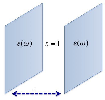
Figure 1: “Casimir” entanglement entropy ${\cal S_{R}}$ of plates.

Consider a field interacting with a medium, defined through the following (Wick rotated) action:

$$S_{\text{pure}}=\frac{1}{2}\int_{-\infty}^{\infty}\frac{d\omega}{2\pi}\Big{\{}\int d^{3}x[\phi^{*}\left(-\omega^{2}+\nabla^{2}\right)\phi_{\omega}]-$$

$$\int_{B}d^{3}x[\frac{\left(\omega^{2}+\omega_{0}{}^{2}\right)}{8\pi^{2}}\psi_{\omega}{}^{*}\psi_{\omega}+\omega_{p}\omega(\psi_{\omega}{}^{*}\phi_{\omega}+\psi_{\omega}\phi_{\omega}{}^{*})]\Big{\}}$$ (15)

where $\psi$ is a matter field which is confined to the body(s) $B$. This action may be viewed as a purification of the state $\rho_{\phi}$ of $\phi$, i.e. we write our state as $\rho_{\phi}={\rm Tr}_{\psi}|\Omega\rangle\langle\Omega|$ for some pure state $|\Omega\rangle$ in the larger $\phi,\psi$ space. The action (The Entanglement of a Quantum Field with a Dispersive Medium) corresponds to the form $\chi(\omega)=\frac{\omega_{p}{}^{2}}{\omega_{0}{}^{2}-\omega^{2}}$ of the response of $\phi$ to a transparent, but dispersive medium.

Finally, to render the problem exactly solvable, we will assume that the $\phi\psi$ coupling in (The Entanglement of a Quantum Field with a Dispersive Medium) comes from the form $\omega_{p}\int\psi\dot{\phi}$ in the classical Lagrangian. Note, that while on the classical level this Lagrangian coupling is equivalent to $-\omega_{p}\int\phi\dot{\psi}$, the actual quantum mechanical transformation required to affect this for gauge fields is of the Power-Zineau-Wooley (PZW) type used to interchange the minimal coupling ${\bf A\cdot J}$ to ${\bf E\cdot P}$ in quantum electrodynamics Cohen-Tannoudji et al. (2004). However, PZW mixes radiation and dipole degrees of freedom and does not preserve entanglement properties.

To compute the entropy of the field $\phi$ more efficiently, we use that ${\cal S}_{\phi}={\cal S}_{\psi}$ (noting that (The Entanglement of a Quantum Field with a Dispersive Medium) describes a pure state). ${\cal S}_{\psi}$ is obtained from the effective action for $\psi$:

$$S_{\text{eff}}[\psi]=-\frac{1}{4\pi}\int_{B}d^{3}xd^{3}x^{\prime}[\omega_{p}^{2}\omega^{2}\langle{\bf x}|G_{0}^{B}|{\bf x}^{\prime}\rangle+$$

$$\delta({\bf x}-{\bf x}^{\prime})\frac{\omega^{2}+\omega_{0}{}^{2}}{8\pi^{2}}]\psi_{\omega}{}^{*}({\bf x})\psi_{\omega}{}^{*}({\bf x}^{\prime}),$$ (16)

where $G_{0}^{B}$ is the restriction of the free Green’s function $G_{0}=\frac{1}{-\omega^{2}+\nabla^{2}}$ to the bodies $B$.

The two point function of $\psi$ is:

$$\langle\psi({\bf x})\psi({\bf x}^{\prime})\rangle=\int_{0}^{\infty}\langle{\bf x}|\frac{1}{\frac{\omega^{2}+\omega_{0}{}^{2}}{8\pi^{2}}+\omega_{p}{}^{2}\omega^{2}G_{0}^{B}}|{\bf x}^{\prime}\rangle{d\omega\over 2\pi}$$ (17)

with a similar expression holding for the conjugate momentum of $\psi$ (obtained from the Lagrangian in $S_{\text{pure}}$):

$${\cal H}_{{\bf x}{\bf x}^{\prime}}=\langle\pi_{\psi({\bf x})}\pi_{\psi({\bf x}^{\prime})}\rangle=-{1\over 16\pi^{4}}$$

$$\int_{0}^{\infty}\langle{\bf x}|\frac{\omega^{2}}{\frac{\omega^{2}+\omega_{0}{}^{2}}{8\pi^{2}}+\omega_{p}{}^{2}\omega^{2}G_{0}^{B}}-8\pi^{2}\delta({\bf x}-{\bf x}^{\prime})|{\bf x}^{\prime}\rangle{d\omega\over 2\pi}$$ (18)

Next, we study the entropy generated by parallel planes separated by a distance $L$, as illustrated in Fig.1. To control UV behavior we place the system on a lattice, and use the discrete analogue of the free Green’s function (in 1D) as: $G_{0}(n,m,k_{\perp})=\frac{e^{-q|n-m|}}{2\sinh q}$, where: $\cosh q=1+\frac{\omega^{2}+{k_{\perp}^{2}}}{2}$ ($k_{\perp}$ is parallel to the plates).

We first consider the 1D case. In 1D, the planes reduce to a pair of sites, and the kernel $(\frac{\omega^{2}+\omega_{0}{}^{2}}{8\pi^{2}}+\omega_{p}{}^{2}\omega^{2}G_{0}^{B})^{-1}$ in eqs. (17,The Entanglement of a Quantum Field with a Dispersive Medium) is a 2X2 matrix, amenable to an analytic treatment. Estimating the two point functions (17) and (The Entanglement of a Quantum Field with a Dispersive Medium) using Watson’s lemma, we find, at large distances $L\gg 1$ (assuming $\omega_{0}>\omega_{p}$ and up to order $\omega_{p}^{2}$):

$${\cal G}_{nm}=\langle\psi(n)\psi(m)\rangle\sim{1\over 2\pi}\left(\begin{array}[]{cc}A_{G}&-\frac{32\text{ }\pi^{4}\omega_{p}{}^{2}}{\omega_{0}{}^{4}L^{2}}\\ -\frac{32\text{ }\pi^{4}\omega_{p}{}^{2}}{\omega_{0}{}^{4}L^{2}}\text{ }&A_{G}\end{array}\right);$$ (21)

$$A_{G}=\frac{4\pi^{3}}{\omega_{0}}-\frac{32\pi^{4}\omega_{p}^{2}(\omega_{0}^{2}\arccos[\frac{2}{\omega_{0}}]-2\sqrt{\omega_{0}^{2}-4})}{\omega_{0}^{2}(\omega_{0}^{2}-4)^{3/2}}.$$ (22)

Similarly, the momentum correlation function ${\cal H}_{nm}$ is

$${\cal H}_{nm}\sim\frac{-1}{32\pi^{5}}\left(\begin{array}[]{cc}A_{H}&-\frac{192\pi^{4}\omega_{p}^{2}}{\omega_{0}^{4}L^{4}}\\ -\frac{192\pi^{4}\omega_{p}^{2}}{\omega_{0}^{4}L^{4}}&A_{H}\end{array}\right);$$ (25)

$$A_{H}={\omega_{0}\over 4\pi}+\frac{32\pi^{4}\omega_{p}^{2}\left(2\sqrt{\omega_{0}^{2}-4}+(\omega_{0}^{2}-8)\arccos[\frac{2}{\omega_{0}}]\right)}{(\omega_{0}^{2}-4)^{3/2}}.$$

The dominant terms in the product $\cal{GH}$ are proportional to $\theta\equiv\frac{1}{64\pi^{6}}A_{G}A_{H}$, and are independent of distance.

As expected on physical grounds, the entropy strongly depends on the pinning frequency $\omega_{0}$. We note that the entropy is maximized when $\omega_{0}$ is small as possible, i.e. $\omega_{0}\sim\omega_{p}$. In this limit the $\psi$ field is only weakly restrained to $\psi=0$ values, and thus generates large entropy for the $\phi$ field. In the weak coupling limit $\omega_{p}\ll 1$ we find the eigenvalues of $\cal{GH}$ to behave as $\theta\left(\omega_{0}=\omega_{p}\right)\sim\frac{1}{4}+2\pi\omega_{p}\log\frac{4}{e\omega_{p}}$. In the opposite limit, when $\omega_{0}\gg\omega_{p}$ the $\psi$ field is essentially “pinned” down, and we have $\theta\sim\frac{1}{4}+\frac{8\pi\omega_{p}^{2}}{\omega_{0}^{3}}-\frac{8\left(\pi^{2}\omega_{p}^{2}\right)}{\omega_{0}^{4}}.$ As $\omega_{0}\rightarrow\infty$ we recover the minimal possible value of the product ${\cal G}{\cal H}$ allowed by the uncertainty principle.

Finally, the symplectic eigenvalues of the covariance matrix are found, to leading orders in ${1\over L},\omega_{p}$, to be

$$\lambda_{\pm}=\sqrt{\theta}\pm A_{H}\omega_{p}^{2}({4\pi^{2}\omega_{0}^{4}\sqrt{\theta}L^{2}})^{-1}$$ (26)

and the entropy using (5) for large $L$ to behave as:

$${\cal S}_{\phi}={\cal S}(L\rightarrow\infty)+32\pi^{7}\omega_{p}^{2}\omega_{0}^{-3}L^{-4}.$$ (27)

At dimensions $D>1$, the momentum $k_{\perp}$ is a good quantum number. We proceed to compute the entropy per $k_{\perp}$ by estimating $\langle\psi(x,k_{\perp})\psi(x^{\prime},k_{\perp})\rangle$ and $\langle\pi_{\psi(x,k_{\perp})}\pi_{\psi(x^{\prime},k_{\perp})}\rangle$. We find that the $L$ dependent, off-diagonal elements in (21,25) are exponentially decaying as $e^{-L|k_{\perp}|}$. Integrating over $k_{\perp}$ yields

$${\cal S}_{\phi}={\cal S}(L\rightarrow\infty)+{C_{d}(\omega_{0},\omega_{p})}{L^{-3-d}}$$ (28)

where $C_{d}(\omega_{0},\omega_{p})$ is a constant.

Discussion: We studied the quantum state of a field in the presence of a dielectric material. We found that such a field is described by a density matrix whose Von-Neumann entropy diverges as described by eq. (12). The state cannot be considered as thermal, but rather the photons have a $k$ dependent effective temperature. The occupation number of modes behaves as $n_{k}\sim 1/\sqrt{k}$ per unit volume for ”soft” photons. A similar situation may arise when considering the phonons in solid. This effect is reminiscent of the infra red problem in quantum electrodynamics where, infinite numbers of soft photons are generated in transition amplitudes (see, e.g. Kibble (1968)). The situation here is different in that the system is in equilibrium, however we are integrating over dipole transitions in the material.

To find long distance features, unaffected by UV divergence, we considered $\cal{S}_{R}$, the distance dependent part of the entropy of two objects. In eq. (The Entanglement of a Quantum Field with a Dispersive Medium) we present a novel general formula for the ”Casimir Entanglement Entropy”. Finally, we considered a toy model for the entropy generated in the field due to interaction between two thin planes. In this model $\cal{S}_{R}$ shows a $L^{-(3+d)}$ decay: Thus, the field matter EE is reduced when the objects are far. Further investigation is needed to determine the power law in more realistic models.

The measurement of the full quantum entropy is, in general, quite hard, but possible to achieve in certain situations Klich et al. (2006); Klich and Levitov (2009); Song et al. (2011); Cardy (2011). In the case of Gaussian fields with translational invariance, it can be computed from mode occupations. We mention that many of the properties discussed are also valid for other fields, such as phonons in a solid. For example, occupation numbers of phonons in ultracold atoms or trapped ion systems may be measurable in experiments Dutta et al. (2011); Brahms et al. (2011), and may reveal some of the features described here.

Financial support from NSF CAREER award No. DMR-0956053 is gratefully acknowledged.

References

- Lifshitz and Pitaevskii (1984) E. M. Lifshitz and L. P. Pitaevskii, Statistical Mechanics, Part 2 (Pergamon, Oxford, 1984).
- Levin and Rytov (1967) M. Levin and S. Rytov, Science, Moscow 6 (1967).
- Amico et al. (2008) L. Amico, R. Fazio, A. Osterloh, and V. Vedral, Rev. Mod. Phys. 80, 517 (2008), URL http://link.aps.org/doi/10.1103/RevModPhys.80.517.
- Caldeira and Leggett (1981) A. Caldeira and A. Leggett, Phys. Rev. Lett. 46, 211 (1981).
- Le Hur (2008) K. Le Hur, Annals of Physics 323, 2208 (2008).
- Lambert et al. (2004) N. Lambert, C. Emary, and T. Brandes, Physical review letters 92, 73602 (2004).
- Marcovitch et al. (2009) S. Marcovitch, A. Retzker, M. Plenio, and B. Reznik, Physical Review A 80, 012325 (2009).
- Calabrese et al. (2009) P. Calabrese, J. Cardy, and E. Tonni, J. of Stat. Phys. 2009, P11001 (2009).
- Li and Haldane (2008) H. Li and F. Haldane, Physical Review Letters 101, 10504 (2008).
- Qi et al. (2011) X. Qi, H. Katsura, and A. Ludwig, Arxiv preprint arXiv:1103.5437 (2011).
- Botero and Reznik (2003) A. Botero and B. Reznik, Phys. Rev. A 67, 052311 (2003).
- Plenio and Virmani (2007) M. Plenio and S. Virmani, Quant. Inf. Comp. 7, 1 (2007).
- Bezerra et al. (2004) V. Bezerra, G. Klimchitskaya, V. Mostepanenko, and C. Romero, Physical Review A 69, 022119 (2004).
- Decca et al. (2005) R. Decca, D. López, E. Fischbach, G. Klimchitskaya, D. Krause, and V. Mostepanenko, Annals of Physics 318, 37 (2005).
- Brevik et al. (2005) I. Brevik, J. Aarseth, J. Høye, and K. Milton, Physical Review E 71, 056101 (2005).
- Sushkov et al. (2011) A. O. Sushkov, W. J. Kim, D. A. R. Dalvit, and S. K. Lamoreaux, Nat. Phys. 7, 230 (2011).
- Geyer et al. (2005) B. Geyer, G. Klimchitskaya, and V. Mostepanenko, Phys.Rev. D72, 085009 (2005).
- Bordag and Pirozhenko (2010) M. Bordag and I. Pirozhenko, Phys. Rev. D. 82, 125016 (2010).
- Feinberg et al. (2001) J. Feinberg, A. Mann, and M. Revzen, Annals of Physics 288, 103 (2001).
- Kenneth and Klich (2006) O. Kenneth and I. Klich, Physical Review Letters 97, 160401 (2006).
- Emig et al. (2007) T. Emig, N. Graham, R. Jaffe, and M. Kardar, Physical Review Letters 99, 170403 (2007).
- Milton and Wagner (2008) K. Milton and J. Wagner, Journal of Physics A: Mathematical and Theoretical 41, 155402 (2008).
- Kenneth and Klich (2008) O. Kenneth and I. Klich, Physical Review B 78, 14103 (2008).
- Cohen-Tannoudji et al. (2004) C. Cohen-Tannoudji, J. Dupont-Roc, and G. Grynberg, Photons and Atoms: Introduction to Quanturn Electrodynamics (Wiley, 2004).
- Kibble (1968) T. Kibble, Journal of Mathematical Physics 9, 315 (1968).
- Klich et al. (2006) I. Klich, G. Refael, and A. Silva, Physical Review A 74, 32306 (2006).
- Klich and Levitov (2009) I. Klich and L. Levitov, Phys. Rev. Lett. 102, 100502 (2009).
- Song et al. (2011) H. Song, C. Flindt, S. Rachel, I. Klich, and K. Le Hur, Physical Review B 83, 161408 (2011).
- Cardy (2011) J. Cardy, Physical Review Letters 106, 150404 (2011).
- Dutta et al. (2011) T. Dutta, M. Mukherjee, and K. Sengupta, Arxiv preprint arXiv:1201.0064 (2011).
- Brahms et al. (2011) N. Brahms, T. Botter, S. Schreppler, D. Brooks, and D. Stamper-Kurn, Arxiv preprint arXiv:1109.5233 (2011).