Single-ion anisotropy in Haldane chains and form factor of the O(3) nonlinear sigma model

Abstract

We consider spin-1 Haldane chains with single-ion anisotropy, which exists in known Haldane chain materials. We develop a perturbation theory in terms of anisotropy, where the magnon-magnon interaction is important even in the low temperature limit. The exact two-particle form factor in the O(3) nonlinear sigma model leads to quantitative predictions on several dynamical properties, including the dynamical structure factor and electron spin resonance frequency shift. These agree very well with numerical results, and with experimental data on the Haldane chain material Ni(C₅H₁₄N₂)₂N₃(PF₆).

One-dimensional quantum spin systems are an ideal subject to test sophisticated theoretical concepts against experimental reality. Giamarchi (2004) One of the best examples is the Haldane gap problem. Haldane predicted in 1983 (Ref. Haldane, 1983) that the standard Heisenberg antiferromagnetic (HAF) chain $\mathcal{H}=J\sum_{j}\bm{S}_{j}\cdot\bm{S}_{j+1}$ has a non-zero excitation gap and exponentially decaying spin-spin correlation function for an integer spin quantum number $S$. It has been long known that the HAF chain with $S=1/2$ is exactly solvable by a Bethe ansatz, and that it has gapless excitations and the power-law spin-spin correlation function. While the same model cannot be solved exactly for $S\geq 1$, Haldane’s prediction was rather unexpected and surprising at the time.

Haldane’s argument was based on the mapping of the HAF chain to the O(3) nonlinear sigma model (NLSM), which is a field theory defined by the action

$$\mathcal{A}_{0}=\frac{1}{2g}\int dtdx\,\biggl{[}\frac{1}{v}(\partial_{t}\bm{n})^{2}-v(\partial_{x}\bm{n})^{2}\biggr{]}+i\theta Q,$$ (1)

where $g=2/S$ is coupling constant, $v$ is spin-wave velocity, $\theta=2\pi S$ and $Q=(1/4\pi)\int dtdx\,\bm{n}\cdot\partial_{t}\bm{n}\times\partial_{x}\bm{n}$ is an integer-valued topological charge. The field $\bm{n}(x)$ is related to the spin $\bm{S}_{j}$ via $\bm{S}_{j}\approx(-1)^{j}\sqrt{S(S+1)}\,\bm{n}(x)+\bm{L}(x)$, where $\bm{L}(x)=\bm{n}\times\partial_{t}\bm{n}/g$. The field $\bm{n}$ has a constraint $\bm{n}^{2}=1$. For a half-integer $S$, the topological term $i\theta Q$ should be kept. However, for an integer $S$, the topological term $i\theta Q=2\pi i\times(\text{integer})$ is irrelevant and it suffices to drop $i\theta Q$ in eq. (1). The O(3) NLSM without the topological term is a massive field theory, which implies that the integer $S$ HAF chain (Haldane chain) has a non-zero gap and a finite correlation length. The Haldane’s conjecture is now confirmed by a large body of theoretical, numerical, and experimental studies. Affleck (1989) Moreover, the O(3) NLSM is also useful in describing integer $S$ HAF chains.

There are various complications in real materials. A Haldane chain material generally has a single-ion anisotropy (SIA): $\mathcal{H}^{\prime}=\sum_{j}[D(S^{z}_{j})^{2}+E\{(S^{x}_{j})^{2}-(S^{y}_{j})^{2}\}]$. This interaction is important, for example, for electron spin resonance (ESR) measurements. ESR is a useful experimental probe which can detect even very small anisotropies. In other words, the anisotropic interaction is the key to understanding a rich store of ESR experimental data. However, the theory of ESR is not sufficiently developed for many systems, including Haldane chains, leaving many experimental data not being understood. In order to fully exploit the potential of ESR, accurate formulation of the SIA in Haldane chains is required.

The SIA can be treated as a perturbation since it is usually small compared to the isotropic exchange interaction $J$. In the O(3) NLSM language, the perturbation is written as

$$\mathcal{H}^{\prime} =S(S+1)\int dx\bigl{[}D(n^{z})^{2}-E\{(n^{x})^{2}-(n^{y})^{2}\}\bigr{]},$$ (2)

which spoils the integrability of the O(3) NLSM. Several simple calculations have been done based on the Landau-Ginzburg (LG) model. Affleck (1991, 1992) When the elementary excited particles (magnons) are dilute, the interaction between magnons may be ignored. If this is the case, the system is effectively described by a much simpler theory of free massive magnons (the LG model). Affleck (1991) However, description by the LG model is not accurate and, furthermore, it is phenomenological. Essler and Affleck (2004) Even in the low-energy limit, where the free magnon approximation is supposed to be exact, it is not the case with respect to the evaluation of Eq. (2). This is because the perturbation (2) creates and annihilates two magnons at the same point; in such a situation, interaction among the magnons is indeed important even when the average density of magnons in the entire system is infinitesimal. Therefore, correct handling of the SIA in the O(3) NLSM framework requires a proper inclusion of the magnon interaction.

In this paper, we present such a formulation, utilizing the integrability of the O(3) NLSM. The effects of interaction are encoded in the form factors of operators. The form factors in integrable field theories can be determined by the consistency with the exact $S$-matrices and several additional axioms. Karowski and Weisz (1978); Berg et al. (1979); Smirnov (1992) Form factor expansion (FFE) is particularly powerful in massive field theories such as the O(3) NLSM, because the higher-order contributions survive only above the higher energy thresholds. Essler and Konik (2005) The leading contribution to the FFE of Eq. (2) is given by the two-particle form factor. The FFE shows an excellent agreement with the correlation function of $(S^{z})^{2}$ numerically obtained in the $S=1$ HAF chain, demonstrating the importance of the interaction. At the same time, the renormalization factor for the SIA (2) is determined by the fitting of the numerical data. Furthermore, we discuss two applications to physical problems of interest: the split of triplet magnons in the dynamical structure factor and the ESR shift in the $S=1$ HAF chain with SIA. We find very good agreement with numerical results in both applications, and with experimental data on the ESR shift, without introducing any extra fitting parameter.

A single magnon excitation can be parametrized by the rapidity $\theta$, so that its energy and wavenumber are given respectively as $\Delta_{0}\cosh\theta$ and $(\Delta_{0}/v)\sinh\theta$, where $\Delta_{0}=0.41J$ is the Haldane gap. Because of interactions among magnons,the $S$ matrix of O(3) NLSM has a complicated structure. Zamolodchikov and Zamolodchikov (1978) The one-particle form factor of an operator $\mathcal{O}$ is defined as a matrix element which connects the ground state $|0\rangle$ to a one-particle state $|\theta_{1},a_{1}\rangle$ ($a_{1}=1,2,3$), namely $F_{\mathcal{O}}(\theta_{1},a_{1})\equiv\langle 0|\mathcal{O}|\theta_{1},a_{1}\rangle$. And the $n$-particle form factor is defined as $F_{\mathcal{O}}(\theta_{1},a_{1};\theta_{2},a_{2};\cdots;\theta_{n},a_{n})\equiv\langle 0|\mathcal{O}|\theta_{1},a_{1};\theta_{2},a_{2};\cdots;\theta_{n},a_{n}\rangle$, where this $n$-particle state is normalized as $\langle\theta^{\prime}_{1},a^{\prime}_{1};\cdots;\theta^{\prime}_{n},a^{\prime}_{n}|\theta_{1},a_{1};\cdots;\theta_{n},a_{n}\rangle=(4\pi)^{n}\delta_{a^{\prime}_{1},a_{1}}\cdots\delta_{a^{\prime}_{n},a_{n}}\delta(\theta^{\prime}_{1}-\theta_{1})\cdots\delta(\theta^{\prime}_{n}-\theta_{n})$.

The FFE of the fundamental field $n^{a}$, which corresponds to (a staggered part of) the spin operator $S^{a}$, has often been studied. The leading contribution to the FFE is the one-particle form factor $F_{n^{a}}(\theta_{1},a_{1})$. Because $n^{a}$ is odd under the transformation $\bm{n}\rightarrow-\bm{n}$, the next order contribution comes from the three-particle form factor, which gives small corrections to the spin-spin correlation function. Horton and Affleck (1999); Essler (2000) On the other hand, the composite operator $(S^{a})^{2}$, which is of our central interest, has been less studied. Since it is proportional to $(n^{a})^{2}$ and even under the reversal $\bm{n}\rightarrow-\bm{n}$, the leading contribution to the FFE comes from the two-particle form factor $F_{(n^{a})^{2}}(\theta_{1},a_{1};\theta_{2},a_{2})$. We note that the exact two-particle form factor of the antisymmetric field $\bm{L}(x)$ in the O(3) NLSM has been applied to describe the uniform part of the spin-spin correlation function of HAF chains. White and Affleck (2008); Sørensen and Affleck (1994, 1994); Affleck and Weston (1992); Konik (2003) Including the renormalization factors for spin operators, which are undetermined at this point, we have

$$F_{S^{a}}(\theta_{1},a_{1}) =\sqrt{Z}\,\delta_{a,a_{1}},$$ (3)

$$F_{(S^{a})^{2}}(\theta_{1},a_{1};\theta_{2},a_{2}) =-iZ_{2}\,\delta_{a_{1},a_{2}}(3\delta_{a,a_{1}}-1)\psi_{2}(\theta_{1}-\theta_{2}).$$ (4)

The two-particle form factor (4) receives contributions from higher-order terms in the FFE of $S^{a}$, and cannot be determined by Eq. (3) alone. Thus $Z_{2}$ is a parameter independent of $Z$.

We have the constraint $\sum_{a=1,2,3}(S^{a})^{2}=2$ on the composite operator. From this constraint and the O(3) symmetry, it follows that $\sum_{a=1,2,3}F_{(S^{a})^{2}}(\theta_{1},3;\theta_{2},3)=\langle 0|\theta_{1},3;\theta_{2},3\rangle=0$, which is satisfied by (4). Integral representation of $\psi_{2}(\theta)$ is given in Ref. Balog and Weisz, 2007, for O($N$) NLSM with a general integer $N$. For $N=3$, it reads

$$\psi_{2}(\theta)=\sinh\frac{\theta}{2}\,\exp\left[\int_{0}^{\infty}\frac{d\omega}{\omega}e^{-\pi\omega}\frac{\cosh[(\pi+i\theta)\omega]-1}{\sinh(\pi\omega)}\right].$$

This integral can be analytically carried out to give

$$\psi_{2}(\theta)=\frac{i}{2}(\theta-\pi i)\tanh\frac{\theta}{2}.$$ (5)

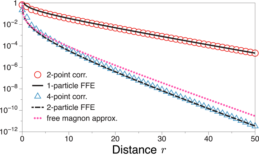
Figure 1: (color online): Numerically calculated spin-spin correlation $(-1)^{r}\langle 0|S^{z}(r)S^{z}(0)|0\rangle$ (circles) and the correlation $\langle 0|(S^{z}(r))^{2}(S^{z}(0))^{2}|0\rangle-4/9$ (triangles) are compared with FFEs (6) with $Z=1.26$ (solid curve) and the connected part of (7) with $Z_{2}=0.24$ (dashed curve). The free magnon approximation (dotted curve) cannot fit the correlation function of $(S^{z})^{2}$.

Determination of the renormalization factors $Z$ and $Z_{2}$ requires numerical calculations. In order to test the validity of the FFE for $(S^{a})^{2}$ and further to determine $Z_{2}$, we computed the equal-time correlation function $\langle 0|(S^{z}(r))^{2}(S^{z}(0))^{2}|0\rangle$ by the infinite time-evolving block decimation (iTEBD) method, Vidal (2007) as shown in Fig. 1.

FFE is derived by inserting the identity $\hat{1}=\sum_{n=0}^{\infty}P_{n}$, where the $P_{n}$’s are the projection operators to the $n$-particle subspace of the Fock space, defined by $P_{0}=|0\rangle\langle 0|$ and $P_{n}=\frac{1}{n!}\sum_{a_{1},\cdots,a_{n}}\int\frac{\prod_{j}d\theta_{j}}{(4\pi)^{n}}|\theta_{1},a_{1};\cdots;\theta_{n},a_{n}\rangle\langle\theta_{1},a_{1};\cdots;\theta_{n},a_{n}|$ for $n\geq 1$. In the leading nonvanishing order, we find

$$(-1)^{r}\langle 0|S^{z}(r)S^{z}(0)|0\rangle\approx Z\int\frac{d\theta}{4\pi}\,e^{i\Delta_{0}r\sinh\theta/v},$$ (6)

$$\langle 0|(S^{z}(r))^{2}(S^{z}(0))^{2}|0\rangle-\frac{4}{9}$$

$$\approx 3{Z_{2}}^{2}\int\frac{d\theta_{1}d\theta_{2}}{(4\pi)^{2}}|\psi_{2}(\theta_{1}-\theta_{2})|^{2}e^{i\Delta_{0}r(\sinh\theta_{1}+\sinh\theta_{2})/v}.$$ (7)

$Z=1.26$ was given in Ref. Sørensen and Affleck (1994) by comparing numerically obtained spin-spin correlation function with the LG model. Concerning the spin-spin correlation function, the LG model is equivalent to the lowest-order FFE (6); our iTEBD calculation also reproduces the result of Ref. Sørensen and Affleck, 1994. On the other hand, to the best of our knowledge, $Z_{2}$ has not been determined previously.

As shown in Fig. 1, the lowest order of FFE (7) shows an excellent agreement with the numerical data; the fit also determines

$$Z_{2}=0.24.$$ (8)

Since we used the known values of the Haldane gap $\Delta_{0}=0.41J$ and the spin-wave velocity $v=2.49J$ (Ref. Todo and Kato, 2001) for $S=1$, the renormalization factor $Z_{2}$ is the only fitting parameter.

In contrast to the FFE (7), the LG model, which ignores interaction among magnons, shows discrepancy with the numerical data, as also shown in Fig. 1. To illustrate the effect of the interaction, let us discuss the asymptotic long-distance behavior of Eqs. (6) and (7). When $r\to+\infty$, only the behavior of $\psi_{2}(\theta)$ at $\theta\sim 0$ is relevant in (7). Here we can expand (6) and (7) as $(-1)^{r}\langle 0|S^{z}(r)S^{z}(0)|0\rangle\propto e^{-r/\xi}/\sqrt{8\pi r/\xi}$ and $\langle 0|(S^{z}(r))^{2}(S^{z}(0))^{2}|0\rangle-4/9\propto e^{-r/\xi_{2}}/(4\pi r/\xi_{2})$. In a relativistic field theory, the inverse correlation length is equivalent to the lowest excitation energy created by the operator; in fact $\xi=v/\Delta_{0}$. Furthermore, in the LG model, Affleck (1991) $\xi_{2}=\xi/2$ should hold. This is because the composite field $(n^{a})^{2}$ creates two particles, and O(3) NLSM does not contain any bound states. Bergknoff and Thacker (1979) Thus the excitation energy for the two-particle creation would be twice the magnon mass ($2\Delta_{0}$), implying $\xi_{2}=\xi/2$. However, the actual numerical data are inconsistent with this relation: $\xi_{2}=2.75<\xi/2=3.01$. This discrepancy is attributed to the interaction between magnons. Since $(n^{a})^{2}$ creates two magnons at the same point, the actual excitation energy is larger than $2\Delta_{0}$, resulting in $\xi_{2}<\xi/2$.

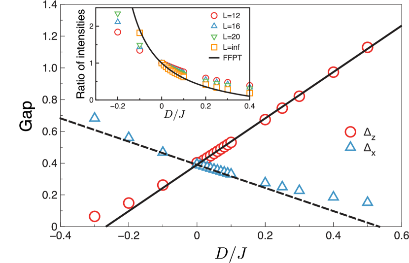
Figure 2: (Color online): Numerically determined excitation gaps $\Delta_{x}$ (circles) and $\Delta_{z}$ (triangles) are plotted for $-0.4\leq D/J\leq 0.6$ and $E=0$. Deviation ofthe numerical data from the first order FFPT (solid and dashed lines) is attributed to higher-order perturbations. Inset: The ratio $\mathcal{S}^{zz}(\pi,\Delta_{z})/\mathcal{S}^{xx}(\pi,\Delta_{x})$ obtained by the Lanczos method (symbols) and (14) (solid curve) are compared. The extrapolation to $L=\infty$ is done by fitting the finite-size data for $L=12,14,16,18$ and $20$ with a polynomial of $1/L$.

With the full determination of the two-particle form factor (4), we turn to discussion of dynamical structure factor (DSF) at $T=0$ in Haldane chains with a SIA. The peaks in the DSF reflect the energy of the magnon at a given momentum. Triply degenerate magnon dispersions in the isotropic chain are split due to the SIA. We determine the first-order perturbation to the masses, $\Delta_{a}^{(1)}\equiv\Delta_{a}-\Delta_{0}$, in the form-factor perturbation theory (FFPT) Controzzi and Mussardo (2004):

$$\Delta_{a}^{(1)}\sim\frac{\langle\theta,a|\mathcal{H}^{\prime}|0,a\rangle}{\langle\theta,a|0,a\rangle}.$$ (9)

In fact, both the numerator and the denominator are proportional to $\delta(\theta)$, and Eq. (9) should be understood as the ratio of the coefficients of $\delta(\theta)$. Furthermore, the numerator equals to $F_{\mathcal{H}^{\prime}}(0,a;\theta-\pi i,a)$ because of the crossing symmetry. LeClair and Mussardo (1999) Therefore, (9) reads

$$\Delta_{x}^{(1)} =-\frac{Z_{2}v}{2\Delta_{0}}D-\frac{3Z_{2}v}{2\Delta_{0}}E,$$ (10)

$$\Delta_{y}^{(1)} =-\frac{Z_{2}v}{2\Delta_{0}}D+\frac{3Z_{2}v}{2\Delta_{0}}E,$$ (11)

$$\Delta_{z}^{(1)} =\frac{Z_{2}v}{\Delta_{0}}D.$$ (12)

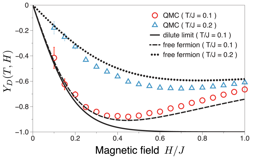
Figure 3: (Color online): Magnetic field dependence of ESR shift $Y_{D}(T,H)$ for $T=0.1J$ (circles) and $T=0.2J$ (triangles). The solid curve is (18), which is exact in $H\to 0$. The dashed and dotted curves are (19) at $T=0.1J$ and $T=0.2J$, respectively.

The leading contribution to the $T=0$ DSF ${\mathcal{S}}^{aa}(\pi,\omega)$ corresponds to the creation of a single magnon. Therefore we find

$${\mathcal{S}}^{aa}(\pi,\omega)\sim\frac{\pi Zv}{\Delta_{a}}\delta(\omega-\Delta_{a}),$$ (13)

which has the identical form to the DSF of a system of free particles. This is natural because the population of magnons approaches zero in the $T\to 0$ limit, and thus the interactions are negligible. Nevertheless, we emphasize that the change of the masses as $\Delta_{a}$ (10)–(12) due to the SIA is affected by the magnon-magnon interaction. Equation (13) implies that the magnon masses $\Delta_{a}$ can be identified with the peak frequency of DSF at the antiferromagnetic wavevector $q=\pi$. In Fig. 2, we compare the magnon masses $\Delta_{a}$ extracted from the $T=0$ DSF peak obtained numerically by the Lanczos method Suzuki and Suga (2005) for various values of $D$ (while setting $E=0$). For small $D$, the numerical data agree very well with the FFPT (10)–(12).

The form of the $T=0$ DSF (13) leads to another prediction: The ratio of the DSF intensities should obey

$$\frac{\int d\omega\;{\mathcal{S}}^{zz}(\pi,\Delta_{z})}{\int d\omega\;{\mathcal{S}}^{xx}(\pi,\Delta_{x})}=\frac{\Delta_{x}}{\Delta_{z}}.$$ (14)

This is also confirmed by the Lanczos data as shown in the inset of Fig. 2.

Let us extend our discussion to the system under a finite magnetic field. Now our Hamiltonian $\mathcal{H}=\mathcal{H}_{0}+\mathcal{H}_{Z}+\mathcal{H}^{\prime}$ consists of three terms. $\mathcal{H}_{0}$ is the SU(2) symmetric exchange interaction, $\mathcal{H}_{Z}=-g_{e}\mu_{B}\bm{H}\cdot\bm{S}=-g_{e}\mu_{B}\bm{H}\cdot\sum_{j}\bm{S}_{j}$ is the Zeeman interaction, and $\mathcal{H}^{\prime}$ is the SIA, which is assumed to be small. $g_{e}$ is Landé $g$ factor of electrons and $\mu_{B}$ is the Bohr magneton. We set $g_{e}\mu_{B}=1$ unless otherwise stated. ESR is a very powerful tool to study the effects of anisotropies on spin dynamics. One of the fundamental quantities in ESR is the resonance frequency shift (ESR shift). The ESR shift is generally given, in the first order of the anisotropy $\mathcal{H}^{\prime}$, as Kanamori and Tachiki (1962); Nagata and Tazuke (1972); Maeda and Oshikawa (2005)

$$\delta\omega=-\frac{\langle[[\mathcal{H}^{\prime},S^{+}],S^{-}]\rangle_{0}}{2\langle S^{z}\rangle_{0}}.$$ (15)

$\langle\cdots\rangle_{0}$ denotes the average with respect to the unperturbed Hamiltonian $\mathcal{H}^{(0)}=\mathcal{H}_{0}+\mathcal{H}_{Z}$. For the SIA, (15) reads $\delta\omega=f(\Theta,\Phi)\,Y_{D}(T,H)$, where $f(\Theta,\Phi)=D(1-3\cos^{2}\Theta)-3E\sin^{2}\Theta\cos 2\Phi$ and

$$Y_{D}(T,H)=\frac{\sum_{j}\langle 3(S^{z}_{j})^{2}-2\rangle_{0}}{2\langle S^{z}\rangle_{0}}.$$ (16)

$(\Theta,\Phi)$ is the polar coordinate of the magnetic field axis.

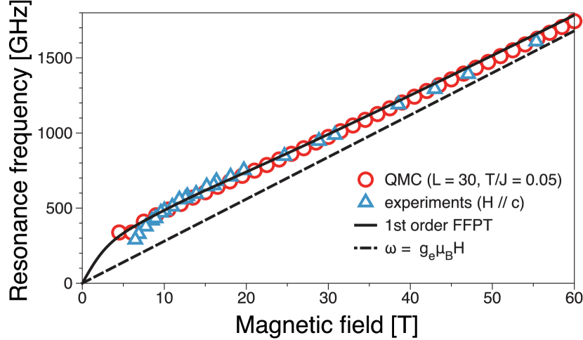
Figure 4: (Color online) Comparison of the resonance frequency $\omega_{\mathrm{r}}=g_{e}\mu_{B}H+\delta\omega$ by QMC (circles) with experimental data Kashiwagi et al. (2009) (triangles). We performed QMC calculations with $L=30$ sites. We used $D=0.25J$ and $H\parallel c$ ($\Theta=\Phi=0$). The solid curve is obtained from (19) and the dashed line represents the paramagnetic resonance $\omega=g_{e}\mu_{B}H$.

To apply the results of the FFPT, first we consider the limit $T,H\ll\Delta_{0}$. Here we could project the numerator to one-magnon subspace, ignoring the multi-magnon contributions. The projection operator is $P_{1}=\int\frac{d\theta}{4\pi}\sum_{a=0,\pm}|\theta,a\rangle\langle\theta,a|$. Note that we introduce a different set of indices $a=0,\pm$ representing magnons with dispersion $E_{a}(\theta)=\Delta_{0}\cosh\theta-aH$. The projection leads to

$$P_{1}\sum_{j}\bigl{[}3(S^{z}_{j})^{2}-2\bigr{]}P_{1}$$

$$=\int\frac{d\theta}{4\pi}\frac{3Z_{2}v}{2\Delta_{0}\cosh\theta}\Bigl{[}2|\theta,0\rangle\langle\theta,0|-|\theta,+\rangle\langle\theta,+|-|\theta,-\rangle\langle\theta,-|\Bigr{]}.$$ (17)

Its thermal expectation value can be given in terms of the (classical) distribution function. Thus we find

$$Y_{D}(T,H) =-\frac{3Z_{2}}{4}\tanh\biggl{(}\frac{H}{2T}\biggr{)}\frac{\int\frac{d\theta}{4\pi}\frac{v}{\Delta_{0}\cosh\theta}e^{-\Delta_{0}\cosh\theta/T}}{\int\frac{d\theta}{4\pi}e^{-\Delta_{0}\cosh\theta/T}}.$$ (18)

Figure 3 shows the magnetic field dependence of $Y_{D}(T,H)$, comparing (18) from the FFPT with the numerical results obtained by (16) with quantum Monte Carlo (QMC) method in ALPS software. Albuquerque et al. (2007)

Although the agreement is good at low temperature $T=0.1J$ and at low magnetic fields $H\ll\Delta_{0}$, the discrepancy is evident for $H\gtrsim\Delta_{0}$. This is rather natural, because the magnon population increases as $H$ is increased, invalidating the dilute limit approximation made in the derivation of Eq. (18). In particular, $T=0$, $H=\Delta_{0}$ is a quantum critical point which separates the low field gapped phase and the high field TLL phase, where magnons are condensed. Although it is difficult to handle the case with nondilute magnons, a reasonable improvement would be incorporating magnon-magnon repulsion through the Pauli exclusion principle by utilizing the Fermi-Dirac distribution function $f_{a}(k)=[e^{\omega_{a}(k)/T}+1]^{-1}$ instead of the classical one, in Eq. (18). This is demonstrated by the fact that the $z=2$ free-fermion theory well describes the low-energy behavior near the quantum critical point $H=\Delta_{0}$. Schulz (1980); Maeda et al. (2007) The magnetization is $\langle S^{z}\rangle=m(T,H)=\int\frac{dk}{2\pi}\bigl{[}f_{+}(k)-f_{-}(k)\bigr{]}$ and $Y_{D}(T,H)$ is

$$Y_{D}(T,H) =\frac{3Z_{2}}{2m(T,H)}\int\frac{dk}{2\pi}\frac{v}{2\omega_{0}(k)}\bigl{[}2f_{0}(k)-f_{+}(k)-f_{-}(k)\bigr{]}.$$ (19)

This reduces to Eq. (18) in the limit $H,T\to 0$. We emphasize that there is no free parameter in our theory since the renormalization factor $Z_{2}$ in the overall coefficient of (19) has been already determined in (8). As shown in Fig. 3, the free-fermion approximation (19) explains the extremum of the ESR shift observed numerically around the critical field $H=\Delta_{0}$.

Figure 4 shows the ESR shift observed experimentally in $\mathrm{Ni(C_{5}H_{14}N_{2})_{2}N_{3}(PF_{6})}$, Kashiwagi et al. (2009) which possesses the SIA, and the corresponding numerical result by the QMC method. Our FFPT (19) successfully accounts for the experimental and numerical results, including the gradual approach to the paramagnetic resonance line $\omega=g_{e}\mu_{B}H$ in the high field region. A dtailed analysis of the ESR shift in the whole range of $H$ will be given in a subsequent publication. Furuya et al.

We thank Seiichiro Suga for giving us the motivation for this study. This work is partly supported by Grant-in-Aid for Scientific Research No. 21540381 (M.O.), the Global COE Program “The Physical Sciences Frontier” (S.C.F.), both from MEXT, Japan, and Grant-in-Aid from JSPS (Grant No.09J08714) (S.T.). M.O. also acknowledges the Aspen Center for Physics where a part of this work was carried out (supported by U.S. NSF Grant No. 1066293). We thank the ALPS project for providing the QMC code. Numerical calculations were performed at the ISSP Supercomputer Center of the University of Tokyo.

References

- Giamarchi (2004) T. Giamarchi, Quantum Physics in One Dimension (Oxford University Press, Oxford, U.K., 2004).
- Haldane (1983) F. D. M. Haldane, Phys. Lett. A, 93, 464 (1983).
- Affleck (1989) I. Affleck, J. Phys.: Condens. Matter, 1, 3047 (1989).
- Affleck (1991) I. Affleck, Phys. Rev. B, 43, 3215 (1991).
- Affleck (1992) I. Affleck, Phys. Rev. B, 46, 9002 (1992).
- Essler and Affleck (2004) F. Essler and I. Affleck, J. Stat. Mech., P12006 (2004).
- Karowski and Weisz (1978) M. Karowski and P. Weisz, Nucl. Phys. B, 139, 455 (1978).
- Berg et al. (1979) B. Berg, M. Karowski, and P. Weisz, Phys. Rev. D, 19, 2477 (1979).
- Smirnov (1992) F. A. Smirnov, Form Factors in Completely Integrable Models of Quantum Field Theory (World Scientific, Singapore, 1992).
- Essler and Konik (2005) F. H. L. Essler and R. M. Konik, in From Fields to Strings: Circumnatigating Theoretical Physics, edited by M. Shifman, A. Vainshtein, and J. Wheater (World Scientific, Singapore, 2005) arXiv:cond-mat/0412421.
- Zamolodchikov and Zamolodchikov (1978) A. B. Zamolodchikov and A. B. Zamolodchikov, Nucl. Phys. B, 133, 525 (1978).
- Horton and Affleck (1999) M. D. P. Horton and I. Affleck, Phys. Rev. B, 60, 11891 (1999).
- Essler (2000) F. Essler, Phys. Rev. B, 62, 3264 (2000).
- White and Affleck (2008) S. R. White and I. Affleck, Phys. Rev. B, 77, 134437 (2008).
- Sørensen and Affleck (1994) E. S. Sørensen and I. Affleck, Phys. Rev. B, 49, 13235 (1994a).
- Sørensen and Affleck (1994) E. S. Sørensen and I. Affleck, Phys. Rev. B, 49, 15771 (1994b).
- Affleck and Weston (1992) I. Affleck and R. Weston, Phys. Rev. B, 45, 4667 (1992).
- Konik (2003) R. M. Konik, Phys. Rev. B, 68, 104435 (2003).
- Balog and Weisz (2007) J. Balog and P. Weisz, Nucl. Phys. B, 778, 259 (2007).
- Vidal (2007) G. Vidal, Phys. Rev. Lett., 98, 070201 (2007).
- Todo and Kato (2001) S. Todo and K. Kato, Phys. Rev. Lett., 87, 47203 (2001).
- Bergknoff and Thacker (1979) H. Bergknoff and H. Thacker, Phys. Rev. D, 19, 3666 (1979).
- Controzzi and Mussardo (2004) D. Controzzi and G. Mussardo, Phys. Rev. Lett., 92, 021601 (2004).
- LeClair and Mussardo (1999) A. LeClair and G. Mussardo, Nucl. Phys. B, 552, 624 (1999).
- Suzuki and Suga (2005) T. Suzuki and S.-i. Suga, Phys. Rev. B, 72, 014434 (2005).
- Kanamori and Tachiki (1962) J. Kanamori and M. Tachiki, J. Phys. Soc. Jpn., 17, 1384 (1962).
- Nagata and Tazuke (1972) K. Nagata and Y. Tazuke, J. Phys. Soc. Jpn., 32, 337 (1972).
- Maeda and Oshikawa (2005) Y. Maeda and M. Oshikawa, J. Phys. Soc. Jpn., 74, 283 (2005).
- Albuquerque et al. (2007) A. Albuquerque, F. Alet, P. Corboz, P. Dayal, A. Feiguin, S. Fuchs, L. Gamper, E. Gull, S. Gürtler, A. Honecker, R. Igarashi, M. Körner, A. Kozhevnikov, A. Läuchli, S. Manmana, M. Matsumoto, I. McCulloch, F. Michel, R. Noack, G. Pawlowski, L. Pollet, T. Pruschke, U. Schollwöck, S. Todo, S. Trebst, M. Troyer, P. Werner, and S. Wessel, J. Mag. Mag. Mat., 310, 1187 (2007).
- Schulz (1980) H. Schulz, Phys. Rev B, 22, 5274 (1980).
- Maeda et al. (2007) Y. Maeda, C. Hotta, and M. Oshikawa, Phys. Rev. Lett., 99, 57205 (2007).
- Kashiwagi et al. (2009) T. Kashiwagi, M. Hagiwara, S. Kimura, Z. Honda, H. Miyazaki, I. Harada, and K. Kindo, Phys. Rev. B, 79, 024403 (2009).
- (33) S. C. Furuya, Y. Maeda, and M. Oshikawa, In preparation.