Wilson’s $6-j$ laws and stitched Markov processes

Abstract.

We show how to insert time into the parameters of the Wilson’s $6-j$ laws to construct discrete Markov chains with these laws. By a quadratic transformation we convert them into Markov processes with linear regressions and quadratic conditional variances. Further conversion into the ”standard form” gives ”quadratic harnesses” with ”classical” value of parameter $\gamma=1\pm 2\sqrt{\sigma\tau}$. For $\gamma=1+2\sqrt{\sigma\tau}$, a random-parameter-representation of the original Markov chain allows us to stitch together two copies of the process, extending time domain of the quadratic harness from $(0,1)$ to $(0,\infty)$.

This is an expanded version with additional details that are omitted from the version intended for publication.

1. Introduction

The work on this paper started with an attempt to fit Markov processes with linear regressions and quadratic conditional variances into Wilson’s $6-j$-laws from [Wil80]. This required choosing appropriate time-parameterization of the laws so that we get a Markov chain, and the appropriate (quadratic) transformation of this chain so that conditional and absolute moments are given by simple enough formulas.

Generically, processes with linear regressions and quadratic conditional variances can be further transformed (”standardized”) so that they are described by five parameters, see [BMW07, Theorem 2.2]. We expected Wilson’s $6-j$ laws to lead to the ”classical” quadratic harnesses with the parameters tied by equality $\gamma=1-2\sqrt{\sigma\tau}$. But, to our surprise, depending on the range of parameters we also got quadratic harnesses with $\gamma=1+2\sqrt{\sigma\tau}$. In the latter case, the initial construction gave only a quadratic harness with time $(0,1)$. However, the underlying Markov chain is a mixture of simpler Markov chains. We used this mixture representation to extend the quadratic harnesses to $(0,\infty)$ by stitching together two conditionally-independent Markov chains with shared randomization. The stitching approach was suggested by the construction of the ”bi-Pascal” process with $\gamma=1+2\sqrt{\sigma\tau}$ in [Jam09]; our argument is modeled on [BW11b].

The paper is organized as follows. In Section 2 we use Wilson $6-j$ laws to construct quadratic harnesses on $(0,1)$ or on $(0,\infty)$, depending on the range of parameter $C$. These are Case 1 and Case 2 of Theorem 2.5. In Section 3 we represent Markov chain from Section 2 as a mixture of ”simpler” Markov chains. We also confirm that each of these Markov chains transforms into a quadratic harness with $\gamma=1$ and $\sigma=0$ (which is our justification for the adjective ”simpler” in the previous sentence.) In Section 4 we stitch together a pair of such quadratic harnesses into the quadratic harness on $(0,\infty)$, thus extending the process from Case 1 of Theorem 2.5 to the maximal time domain.

The expanded version of this paper with additional technical or computational details is posted on the arXiv.

1.1. Quadratic harnesses

In [BMW07] the authors consider square-integrable stochastic processes on $(0,\infty)$ such that for all $t,s>0$,

(1.1) $${\mathbb{E}}(Z_{t})=0,\>{\mathbb{E}}(Z_{s}Z_{t})=\min\{s,t\},$$

and for $s<t<u$, ${\mathbb{E}}({Z_{t}}|{\mathcal{F}_{s,u}})$ is a linear function of $Z_{s},Z_{u}$, and ${\rm Var}[Z_{t}|\mathcal{F}_{s,u}]$ is a quadratic function of $Z_{s},Z_{u}$. Here, $\mathcal{F}_{s,u}$ is the two-sided $\sigma$-field generated by $\{Z_{r}:r\in(0,s]\cup[u,\infty)\}$. Then (1.1) implies that

(1.2) $${\mathbb{E}}({Z_{t}}|{\mathcal{F}_{s,u}})=\frac{u-t}{u-s}Z_{s}+\frac{t-s}{u-s}Z_{u}$$

for all $s<t<u$, which is sometimes referred to as a harness condition, see e. g. [MY05].

While there are numerous examples of harnesses, the assumption of quadratic conditional variance is more restrictive. For example, all integrable Lévy processes are harnesses, but as determined by Wesołowski [Wes93], only a few of them are also quadratic harnesses. Under certain technical assumptions, [BMW07, Theorem 2.2] asserts that quadratic variance has the following form: there exist numerical constants $\eta,\theta,\sigma,\tau,\gamma\in\mathds{R}$ such that for all $s<t<u$,

(1.3) $${\rm Var}[Z_{t}|\mathcal{F}_{s,u}]\\ =\frac{(u-t)(t-s)}{u(1+\sigma s)+\tau-\gamma s}\left(1+\eta\frac{uZ_{s}-sZ_{u}}{u-s}+\theta\frac{Z_{u}-Z_{s}}{u-s}\right.\\ \left.+\sigma\frac{(uZ_{s}-sZ_{u})^{2}}{(u-s)^{2}}+\tau\frac{(Z_{u}-Z_{s})^{2}}{(u-s)^{2}}-(1-\gamma)\frac{(Z_{u}-Z_{s})(uZ_{s}-sZ_{u})}{(u-s)^{2}}\right).$$

Definition 1.1.

We will say that a square-integrable stochastic process $(Z_{t})_{t\in T}$ is a quadratic harness on $T$ with parameters $(\eta,\theta,\sigma,\tau,\gamma)$, if it satisfies (1.1), (1.2) and (1.3) on an open interval $T$ which may be all of or a proper subset of $(0,\infty)$. We also assume that the one-sided conditional moments are as follows: for $0<s\leq t\leq u$ in $T$,

(1.4) $$\mathbb{E}\left[\left.{Z_{t}}\right|{{\mathcal{F}}_{\geq u}}\right]=\frac{t}{u}Z_{u},$$

(1.5) $$\mathbb{E}\left[\left.{Z_{t}}\right|{{\mathcal{F}}_{\leq s}}\right]=Z_{s},$$

(1.6) $$\operatorname{Var}\left[\left.{Z_{t}}\right|{{\mathcal{F}}_{\leq s}}\right] = \frac{t-s}{1+\sigma s}\left(\sigma Z_{s}^{2}+\eta Z_{s}+1\right),$$

(1.7) $$\operatorname{Var}\left[\left.{Z_{t}}\right|{{\mathcal{F}}_{\geq u}}\right] = \frac{t(u-t)}{u+\tau}\left(\tau\frac{Z_{u}^{2}}{u^{2}}+\theta\frac{Z_{u}}{u}+1\right).$$

We remark that on infinite intervals, formulas (1.4-1.7) follow from the other assumptions, see [BMW07, (2.7), (2.8), (2.27), and (2.28)].

We expect that quadratic harnesses on finite intervals are determined uniquely by the parameters. This has been confirmed under some technical assumptions when the parameters satisfy additional constraints, of which the main constraint seem to have been that $-1\leq\gamma\leq 1-2\sqrt{\sigma\tau}$.

It is known, see [BMW07], that for quadratic harnesses on $(0,\infty)$, parameters $\sigma,\tau$ are non-negative, and that $\gamma\leq 1+2\sqrt{\sigma\tau}$. Quadratic harnesses with $\gamma=1-2\sqrt{\sigma\tau}$ were called ”classical” in [BMW07]. Quadratic harnesses with $\gamma=1+2\sqrt{\sigma\tau}$ could also have been called ”classical”, but there had been no examples of such processes until the bi-Pascal process was constructed in [Jam09]. The bi-Pascal process does not have higher moments so large part of general theory developed in [BMW07] does not apply. Our interest here is in providing additional examples of quadratic harnesses with $\gamma=1\pm 2\sqrt{\sigma\tau}$.

2. Quadratic harnesses with finite number of values

A family of quadratic harnesses $(Z_{t})$ with two values appears in [BMW08, Section 3.2]. These processes have parameter $\gamma=-1$ and their trajectories follow two quadratic curves. Since $1,Z_{t},Z_{t}^{2}$ are linearly dependent, the parameters in (1.3) are not determined uniquely. In fact, one can show that for this family of processes the admissible parameters in (1.3) can take any real values $\sigma,\tau\in\mathds{R}$ (positive or negative) such that $\sigma\tau\neq 1$ and any $\eta,\theta\in\mathds{R}$ such that

$$(\eta\tau+\theta)(\eta+\theta\sigma)+\left(1-\sigma\tau\right)^{2}>0.$$

Quadratic harnesses with finite number of values, including two values, appear also in [BW10, Section 4.2]. The processes constructed there have parameter $\gamma<1-\sqrt{\sigma\tau}$.

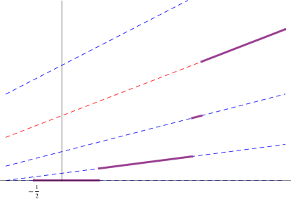
Figure 1. Trajectories of process $(Y_{t})_{t\in\mathcal{T}}$ lie on the family of lines. The process starts at line $\ell_{0}=(A+t)A$, at $t=-A-B$ and jumps up until it stops on a random line $\ell_{\Theta}=(A+t+\Theta)(A+\Theta)$ that it follows to $\infty$. (Here, $A=0,B=1/2,N=4,\Theta=3$; for more on $\Theta$, see (3.14).)

In this section we construct (non-homogeneous) Markov processes which take a finite number of values and we show how to transform them into quadratic harnesses with $\gamma=1\pm 2\sqrt{\sigma\tau}$. These processes are different from the previous ones even in the case of two-values; this can be seen from analyzing the curves they follow, see Figure 1. Somewhat surprisingly, processes corresponding to $\gamma=1\pm\sqrt{\sigma\tau}$ are described by the same formulas for transition probabilities, differing only in the range of one of the parameters that enter the formulas.

Our construction is based on Wilson’s [Wil80] $6-j$ laws. As in [Wil80, (3.5)] we fix integer $N\geq 1$ and assume that

(2.1) $$a>-1/2,\;b\in(-a,a+1),\mbox{ and either $c>a+N$ or $c<-a-N+1$}.$$

(The choice of the range for $c$ will later affect the properties of the quadratic harness.)

For $N\in\mathds{N}$ and $k=0,1,\dots,N$, define

(2.2) $$p_{k,N}(a,b,c)=C_{N}(a,b,c)\frac{(2a)_{k}(a+1)_{k}(a+b)_{k}(a+c)_{k}(-N)_{k}}{k!(a)_{k}(a-b+1)_{k}(a-c+1)_{k}(2a+N+1)_{k}}.$$

where the normalizing constant is

(2.3) $$C_{N}(a,b,c)=\frac{(a-b+1)_{N}(a-c+1)_{N}}{(2a+1)_{N}(-b-c+1)_{N}}$$

and $(a)_{k}=\Gamma(a+k)/\Gamma(a)=a(a+1)\dots(a+k-1)$ is the Pochhammer symbol.

When the parameters are such that numbers $p_{k,N}(a,b,c)$ are well defined, then the sum over all $k=0,\dots,N$ is one; this is [Wil80, formula (3.4)] applied to $m=n=0$. So under assumption (2.1), from [Wil80, (3.4)] one reads out that

(2.4) $$\nu(dx)=\sum_{k=0}^{N}p_{k,N}(a,b,c)\delta_{k}(dx)$$

is a probability measure on $\{0,1,\dots,N\}$.

The following algebraic formula will be used several times.

Lemma 2.1.

For $k=0,1,\dots,N$, $j=0,1,\dots,k$,

(2.5) $$\frac{p_{j,k}(a,b,a+k+2\delta)p_{k,N}(a+\delta,b+\delta,c)}{p_{j,N}(a,b,c+\delta)}=p_{k-j,N-j}(a+j+\delta,-a-j+\delta,c)\;.$$

Proof.

Multiplying both sides of (2.5) by $p_{j,N}(a,b,c+\delta)$, expanding them by the use of (2.2) and (2.3), canceling out common terms and grouping the remaining ones, we observe that (2.5) would follow if we verify that $LHS=RHS$ with

$$LHS=\frac{1}{(2a+1)_{k}(2a+k+1)_{j}}\frac{(2a+2\delta)_{k}(2a+2\delta+k)_{j}}{(2a+2\delta+1)_{N}(2a+2\delta+N+1)_{k}}(a+c+\delta)_{k}\\ \frac{(a+\delta+1)_{k}}{(a+\delta)_{k}}\frac{(-2\delta-k+1)_{k}}{(-2\delta-k+1)_{j}}\frac{(a-c+\delta+1)_{N}}{(a-c+\delta+1)_{k}}\frac{(a+b+2\delta)_{k}}{(-a-b-2\delta-k+1)_{k}}\frac{(-k)_{j}(-N)_{k}}{k!},$$

and

$$RHS=\frac{(2a+2j+1)_{N-j}}{(2a+1)_{N}(2a+N+1)_{j}(2a+2j+1)_{k-j}}\\ \frac{(2a+2\delta+2j)_{k-j}}{(2a+2\delta+2j+1)_{N-j}(2a+2\delta+j+N+1)_{k-j}}(a+c+\delta)_{j}(a+c+\delta+j)_{k-j}\\ \frac{(a+\delta+j+1)_{k-j}}{(a+\delta+j)_{k-j}}(2\delta)_{k-j}\frac{(a-c+\delta+j+1)_{N-j}}{(a-c+\delta+j+1)_{k-j}}\\ \frac{(a-c-\delta+1)_{N}}{(a-c-\delta+1)_{j}(a-c-\delta+j+1)_{N-j}}\frac{(j-N)_{k-j}(-N)_{j}}{(k-j)!}.$$

To perform the verification, we will use the following simplification rules

(2.6) $$(\alpha)_{N}(\alpha+N)_{M} = (\alpha)_{M+N},$$

(2.7) $$\frac{(\alpha+L+1)_{M-L}}{(\alpha+L)_{M-L}} = \frac{\alpha+M}{\alpha+L},$$

(2.8) $$\frac{(\alpha)_{L}}{(\alpha+1)_{M+L}} = \frac{\alpha}{(\alpha+L)_{M+1}}.$$

From (2.6) it follows that

$$\frac{(2a+2j+1)_{N-j}}{(2a+1)_{N}(2a+N+1)_{j}(2a+2j+1)_{k-j}}=\frac{(2a+k+j+1)_{N-k}}{(2a+1)_{N+j}}=\\ \frac{(2a+k+j+1)_{N-k}}{(2a+1)_{k+j}(2a+1+k+j)_{N-k}}=\frac{1}{(2a+1)_{k}(2a+k+1)_{j}}.$$

Similarly, (2.6) and (2.8) give

$$\frac{(2a+2\delta+2j)_{k-j}}{(2a+2\delta+2j+1)_{N-j}(2a+2\delta+j+N+1)_{k-j}}\\ =\frac{(2a+2\delta+2j)_{k-j}}{(2a+2\delta+2j+1)_{N+k-2j}}=\frac{2a+2\delta+2j}{(2a+2\delta+k+j)_{N+1-j}},$$

while applied to the analogous expression in $LHS$ they give

$$\frac{(2a+2\delta)_{k}(2a+2\delta+k)_{j}}{(2a+2\delta+1)_{N}(2a+2\delta+N+1)_{k}}=\frac{(2a+2\delta)_{k+j}}{(2a+2\delta+1)_{k+N}}=\frac{2a+2\delta}{(2a+2\delta+k+j)_{N+1-j}}.$$

From (2.6) we get

$$(a+c+\delta)_{j}(a+c+\delta+j)_{k-j}=(a+c+\delta)_{k},$$

$$\frac{(a-c+\delta+j+1)_{N-j}}{(a-c+\delta+j+1)_{k-j}}=(a-c+\delta+k+1)_{N-k}=\frac{(a-c+\delta+1)_{N}}{(a-c+\delta+1)_{k}},$$

and (this expression appears only in $RHS$)

$$\frac{(a-c-\delta)_{N}}{(a-c-\delta+1)_{j}(a-c-\delta+j+1)_{N-j}}=1.$$

From (2.7) it follows that

$$\frac{(a+\delta+j+1)_{k-j}}{(a+\delta+j)_{k-j}}=\frac{a+\delta+k}{a+\delta+j}\ \textrm{ and }\ \frac{(a+\delta+1)_{k}}{(a+\delta)_{k}}=\frac{a+\delta+k}{a+\delta}.$$

For the remaining expressions from $LHS$ we have

$$\frac{(-2\delta-k+1)_{k}}{(-2\delta-k+1)_{j}}=(-1)^{k+j}(2\delta)_{k-j}\ \mbox{ and }\ \frac{(a+b+2\delta)_{k}}{(-a-b-2\delta-k+1)_{k}}=(-1)^{k}.$$

Now, the above simplifications show that equality $LHS=RHS$ is equivalent to

$$\frac{(-k)_{j}(-N)_{k}}{k!}(-1)^{k+j}(2\delta)_{k-j}\frac{2a+2\delta}{(2a+2\delta+k+j)_{N+1-j}}\frac{a+\delta+k}{a+\delta}(-1)^{k}\\ =\frac{(j-N)_{k-j}(-N)_{j}}{(k-j)!}(2\delta)_{k-j}\frac{2a+2\delta+2j}{(2a+2\delta+k+j)_{N+1-j}}\frac{a+\delta+k}{a+\delta+j},$$

which is easily seen to be true. Thus (2.5) is proved.

∎

In particular, by taking the sum over $j$ in (2.5) we have

(2.9) $$p_{k,N}(a+\delta,b+\delta,c)=\sum_{j=0}^{k}p_{j,N}(a,b,c+\delta)p_{k-j,N-j}(a+j+\delta,-a-j+\delta,c).$$

Next we compute the moments of an auxiliary random variable associated with probability law (2.4).

Proposition 2.2.

Suppose parameters $a,b,c,N$ satisfy (2.1). For $k=0,\dots,N$, consider a random variable $Y$ such that

(2.10) $$\Pr(Y=k(2a+k))=p_{k,N}(a,b,c).$$

Then

(2.11) $${\mathbb{E}}(Y)=\frac{(a+b)(a+c)N}{b+c-N}$$

and

(2.12) $$\operatorname{Var}(Y)=\frac{N(a-b+N)(a+b)(a-c+N)(a+c)(b+c)}{(b+c-N)^{2}(N-b-c-1)}.$$

Proof.

The proof is elementary for $N=0,1$, as the law of $Y$ is $\delta_{0}$ for $N=0$ and

$$\frac{(a-b+1)(a-c+1)}{(2a+1)(-b-c+1)}\delta_{0}+\frac{(a+b)(a+c)}{(2a+1)(b+c-1)}\delta_{2a+1}$$

for $N=1$.

For $N>1$ and $k\geq 1$, we have

$$k(2a+k)p_{k,N}(a,b,c)=\frac{(a+b)(a+c)N}{b+c-N}p_{k-1,N-1}(a+1,b,c)\;,$$

which gives (2.11). For $k>2$, iterating the algebraic identity we get

$$k(k-1)(2a+k)(2a+k+1)p_{k,N}(a,b,c)\\ =\frac{(a+b)(a+b+1)(a+c)(a+c+1)(N-1)N}{(b+c-N)(b+c-N+1)}p_{k-2,N-2}(a+2,b,c).$$

Noting that $k(k-1)(2a+k)(2a+k+1)=k^{2}(2a+k)^{2}-(1+2a)k(2a+k)$, we evaluate

$${\mathbb{E}}(Y^{2})=\frac{(a+b)(a+b+1)(a+c)(a+c+1)(N-1)N}{(b+c-N)(b+c-N+1)}+(1+2a){\mathbb{E}}(Y)$$

and (2.12) follows by an elementary calculation. ∎

2.1. Markov chain

Now we introduce a continuous time (non-homogeneous) Markov chain on the finite state space $\{0,1,\dots,N\}$ with parameters $A$, $B$, $C$. We assume that $N\in\mathds{N}$, $A>-1/2$, $B\in(-A,A+1)$. For the third parameter, we will assume that either

• $C<-A-N+1$,

or

• $C>A+N$.

These two cases will appear in several statements below.

The Markov process will be defined for $t\in\mathcal{T}$, where

$$\mathcal{T}=\begin{cases}\left(-(A+B),\infty\right)&\mbox{ in Case 1,}\\ \left(-(A+B),C-A-N\right)&\mbox{ in Case 2.}\end{cases}$$

We remark that $A+B>0$ and that in Case 2 the interval $\mathcal{T}$ is non-empty, as $C-A-N>0$.

We also remark that the process in Case 1 is well defined on another interval $(-\infty,C-A-N)$. This second ”component” of the process will be used to extend the quadratic harness from $(0,1)$ to $(0,\infty)$. (In fact, one should think that in Case 1, the process starts at $-A-B$ at state $0$, continues through $\infty=-\infty$ and ends at state $N$ at time $C-A-N$.)

For $s<t$ in $\mathcal{T}$, define matrix $P_{s,t}=[p_{s,t}(k,n)]_{0\leq k,n\leq N}$ with entries

(2.13) $$p_{s,t}(k,n)=p_{n-k,N-k}\left(A+\frac{t}{2}+k,-A-s+\frac{t}{2}-k,C-\frac{t}{2}\right)$$

if $0\leq k\leq n\leq N$, and let $p_{s,t}(k,n)=0$ for all other values $k,n\in\{0,\dots,N\}$.

The following shows that matrices $P_{s,t}$ are transition probabilities of a Markov chain.

Proposition 2.3 (Chapman-Kolmogorov equations).

For $s<t<u$ in $\mathcal{T}$, $p_{s,t}(k,n)\geq 0$, and for $j\leq n\leq N$,

(2.14) $$p_{s,u}(j,n)=\sum_{k=j}^{n}p_{s,t}(j,k)p_{t,u}(k,n).$$

Furthermore,

(2.15) $$\sum_{k=j}^{N}p_{s,t}(j,k)=1.$$

Proof.

To verify (2.14), we apply (2.9) with parameters

$$a=A+j+t/2,\;b=-A-j-s+t/2,\;c=C-u/2,\;\delta=(u-t)/2.$$

Formula (2.15) is the already mentioned generic identity for the weights.

To verify that for $0\leq k\leq n\leq N$ we have $p_{s,t}(k,n)\geq 0$ we verify assumption (2.1). Here $a=A+k+t/2$, $b=-A-k-s+t/2$, $c=C-t/2$. We get

$$a=A+k+t/2>(A-B)/2+k>-1/2+k>0$$

as $t>-(A+B)$, $B<A+1$ and $k\geq 0$,

$$b=-A-k-s+t/2=-a+t-s>-a$$

as $t>s$, and

$$a+1-b=2A+1+2k+s>A-B+2k+1>2k>0$$

as $s>-(A+B)$, $B<A+1$ and $k\geq 0$. If $C<-A-N+1$ then

$$c=C-t/2<-A-N+1-t/2=-a-(N-k)+1.$$

If $C>A+N$ then

$$c-a=C-A-k-t>N-k,$$

since $t<C-A-N$.

∎

Let $(\xi_{t})_{t\in\mathcal{T}}$ be the Markov chain constructed above, i.e.

$$\Pr(\xi_{t}=n|\xi_{s}=k)=p_{s,t}(k,n),\,0\leq k\leq n\leq N.$$

In particular, the univariate laws of the Markov chain are

$$\Pr(\xi_{t}=j)=p_{-A-B,t}(0,j)=p_{j,N}(A+t/2,B+t/2,C-t/2).$$

For $t\in\mathcal{T}$, consider the process

(2.16) $$Y_{t}=(2A+t+\xi_{t})\xi_{t}+A(A+t)=(A+t+\xi_{t})(A+\xi_{t}).$$

Lemma 2.4.

$(Y_{t})$ is a Markov process with mean

(2.17) $${\mathbb{E}}(Y_{t})=\frac{A(B+C)(A+N)+NBC}{B+C-N}+t\frac{A(B+C)+NC}{B+C-N}$$

and variance

(2.18) $$\operatorname{Var}(Y_{t})=-\frac{N(A+C)(B+C)(A-B+N)}{(B+C-N)^{2}(B+C-N+1)}(A+B+t)(A-C+N+t).$$

Proof.

The Markov property follows from the fact that the lines $\ell_{k}(t)=(A+t+k)(A+k)$ for $k=0,1,\dots,N$ do not intersect over $t\in\mathcal{T}$. Indeed, $\ell_{k}$ and $\ell_{j}$ intersect at $t=-(2A+j+k)<-2A-1<-(A+B)$. Therefore, the law $\sum p_{t}(k)\delta_{k}$ converges to the degenerate law $\delta_{0}$ as $t\to-(A+B)$ from the right.

The formulas for the mean and the variance are now recalculated from Proposition 2.2, noting that $Y_{t}$ is in distribution $Y+A(A+t)$ with $Y$ given by (2.10). ∎

Of course, $(Y_{t})_{t\in\mathcal{T}}$ naturally extends to the left endpoint by $\lim_{t\to-(A+B)}Y_{t}=-AB$ in mean square and, for a separable version, almost surely.

From Proposition 2.2 we read out that for $s<t$ the conditional moments are

(2.19) $${\mathbb{E}}(Y_{t}|Y_{s})=Y_{s}\frac{A-C+N+t}{A-C+N+s}-\frac{C(A+N)(t-s)}{A-C+N+s},$$

(2.20) $$\operatorname{Var}(Y_{t}|Y_{s})\\ =(A-C+N+t)(t-s)\frac{\left(Y_{s}+C(s-C)\right)\left(Y_{s}-(A+N)(s+A+N)\right)}{(A-C+N+s)^{2}(A-C+N+s-1)}.$$

Indeed, $p_{s,t}(k,n)=p_{n-\xi_{s},N-\xi_{s}}(A+t/2+\xi_{s},-A-s+t/2-\xi_{s},C-t/2)$. Recall

(2.21) $${\rm Cov}(X,Y)={\mathbb{E}}({\rm Cov}(X,Y|U))+{\rm Cov}({\mathbb{E}}(X|U),{\mathbb{E}}(Y|U)).$$

Using (2.21) with $X=U=Y_{s}$, $Y=Y_{t}$, from (2.18) and (2.19) we compute

(2.22) $${\rm Cov}(Y_{s},Y_{t})=\frac{A-C+N+t}{A-C+N+s}\operatorname{Var}(Y_{s})\\ =-\frac{N(A+C)(B+C)(A-B+N)(A+B+s)(A-C+N+t)}{(B+C-N)^{2}(B+C-N+1)}.$$

We now compute the two-sided conditional distribution

$$\Pr(\xi_{t}=j|\xi_{s}=k,\xi_{u}=m)=\frac{\Pr(\xi_{t}=j|\xi_{s}=k)\Pr(\xi_{u}=m|\xi_{t}=j)}{\Pr(\xi_{u}=m|\xi_{s}=k)}=\frac{p_{s,t}(k,j)p_{t,u}(j,m)}{p_{s,u}(k,m)}.$$

The conditional probability is well defined and non-zero only for $k\leq j\leq m\leq N$, and then we have

(2.23) $$\Pr(\xi_{t}=j|\xi_{s},\xi_{u})=p_{j-\xi_{s},\xi_{u}-\xi_{s}}(A+\xi_{s}+t/2,-s+t/2-A-\xi_{s},\xi_{u}+A-t/2+u).$$

Indeed, from (2.5) it follows that

$$\frac{p_{j-k,N-k}(a,b,c+\delta)p_{m-j,N-j}(a+j-k+\delta,-a-j+k+\delta,c)}{p_{m-k,N-k}(a+\delta,b+\delta,c)}\\ =p_{j-k,m-k}(a,b,a+m-k+2\delta).$$

Taking $a=A+t/2+k$, $b=-A-s+t/2-k$, $c=C-u/2$ and $\delta=(u-t)/2$, we get (2.23).

We now use (2.23) to compute the two-sided conditional moments. For fixed $\xi_{s}=k,\xi_{u}=m$, we use (2.11) with $a=A+k+t/2$, $b=-s+t/2-A-k$, $c=m+A-t/2+u$ and $N=m-k$ to compute ${\mathbb{E}}(Y|\xi_{s},\xi_{u})$ where $Y=(\xi_{t}-k)(2a+\xi_{t}-k)$. Since $\Pr(Y_{t}=y|\xi_{s}=k,\xi_{u}=m)=\Pr(Y+(A+k)(A+k+t)=y)$, reverting to $k=\xi_{s}$ and $m=\xi_{u}$, we obtain

$${\mathbb{E}}(Y_{t}|\xi_{s},\xi_{u})=\left(A+\xi_{s}\right)\left(A+t+\xi_{s}\right)\\ +\frac{(t-s)\left(\xi_{u}-\xi_{s}\right)\left(2A+u+\xi_{s}+\xi_{u}\right)}{u-s}\\ =\frac{u-t}{u-s}\xi_{s}(2A+s+\xi_{s})+\frac{t-s}{u-s}\xi_{u}\left(2A+u+\xi_{u}\right)+A(A+t).$$

Hence a calculation based on (2.16) gives

(2.24) $${\mathbb{E}}(Y_{t}|Y_{s},Y_{u})=\frac{(u-t)Y_{s}+(t-s)Y_{u}}{u-s}.$$

Next, we use (2.12) with $N=\xi_{u}-\xi_{s}$, $a=A+\xi_{s}+t/2$, $b=-s+t/2-A-\xi_{s}$, and $c=\xi_{u}+A-t/2+u$ to compute the conditional variance:

$$\operatorname{Var}(Y_{t}|\xi_{s},\xi_{u})\\ =C_{t,s,u}(\xi_{u}-\xi_{s})(\xi_{u}-\xi_{s}+u-s)(2A+s+\xi_{s}+\xi_{u})(2A+u+\xi_{s}+\xi_{u}),$$

where

$$C_{t,s,u}=\frac{(t-s)(u-t)}{(u-s+1)(u-s)^{2}}\;.$$

This gives

(2.25) $$\operatorname{Var}(Y_{t}|Y_{s},Y_{u})=\frac{(u-t)(t-s)}{u-s+1}\left(\frac{(Y_{u}-Y_{s})^{2}}{(u-s)^{2}}-\frac{uY_{s}-sY_{u}}{u-s}\right).$$

The following summarizes our findings and incorporates them as an appropriate transformation into a quadratic harness.

Theorem 2.5.

In Case 1, $(Y_{t})_{t\in\mathcal{T}}$ can be transformed into a quadratic harness $(Z_{t})_{t}$ on $\mathcal{T}^{\prime}=(0,1)$ with covariance (1.1) and the conditional variance (1.3) with parameters

(2.26) $$\eta = -\frac{A(B+C+N)+C(B+C)+N(N-B)}{\sqrt{N(A+C)(B+C)(A-B+N)(N-1-B-C)}},$$

(2.27) $$\theta = -\frac{A(B+C+N)-B(B+C-N)+2CN}{\sqrt{N(A+C)(B+C)(A-B+N)(N-1-B-C)}},$$

(2.28) $$\sigma=\tau = \frac{1}{N-1-B-C},$$

(2.29) $$\gamma = 1+2\sqrt{\sigma\tau}=\frac{B+C-N-1}{B+C-N+1}.$$

In Case 2, $(Y_{t})_{t\in\mathcal{T}}$ can be transformed into a quadratic harness $(Z_{t})_{t}$ on $\mathcal{T}^{\prime}=(0,\infty)$ with parameters

$$\eta = -\frac{A(B+C+N)+C(B+C)+N(N-B)}{\sqrt{N(A+C)(B+C)(A-B+N)(B+C-N+1)}},$$

$$\theta = \frac{A(B+C+N)-B(B+C-N)+2CN}{\sqrt{N(A+C)(B+C)(A-B+N)(B+C-N+1)}},$$

$$\sigma=\tau = \frac{1}{B+C-N+1},$$

and $\gamma=1-2\sqrt{\sigma\tau}=(B+C-N-1)/(B+C-N+1)$.

Proof.

We shall use Proposition A.1. Since Case 1 and Case 2 differ in some details, in order to treat them in a unified way we adopt the convention that $\varepsilon=1$ refers to Case 1, and $\varepsilon=-1$ refers to Case 2. We set

(2.30) $$M=\varepsilon(N-B-C)^{-1}\sqrt{\frac{N(A+C)(B+C)(A-B+N)}{\varepsilon(N-1-B-C)}},$$

noting that the expression under the radical is positive in both cases. Let $\psi=A+B$, $\delta=\varepsilon(A-C+N)$, so that $\delta-\varepsilon\psi=\varepsilon(N-B-C)>0$ in both cases. We take

$$\alpha=\frac{A(B+C)(A+N)+NBC}{B+C-N},\;\beta=\frac{A(B+C)+NC}{B+C-N},$$

$\theta_{0}=0,\eta_{0}=-1$, and define

(2.31) $$X_{t}=Y_{t}-\mathbb{E}Y_{t},\ Z_{t}=m(t)X_{\ell(t)/m(t)},$$

with

(2.32) $$\ell(t)=\frac{t(A-C+N)-\varepsilon(A+B)}{M(N-B-C)}\mbox{ and }m(t)=\frac{\varepsilon-t}{M(N-B-C)}$$

as defined in Proposition A.1. Then by Proposition A.1, $(Z_{t})$ is a quadratic harness, and the formulas follow by calculation. First,

$$\chi=\beta^{2}-\alpha=\frac{(A+C)(B+C)N(A-B+N)}{(B+C-N)^{2}}>0,$$

so

$$M/\chi=-\varepsilon(B+C-N)/\sqrt{\varepsilon(A+C)(B+C)N(A-B+N)(N-1-B-C)},$$

and $\sigma=\tau=\varepsilon/(N-1-B-C)$. Then,

$$\eta=\frac{M(2\beta\varepsilon-\delta)}{\chi}=\frac{\varepsilon M}{\chi}\times\frac{N^{2}+(A-B)N+(A+C)(B+C)}{B+C-N}$$

and

$$\theta=\frac{M(2\beta-\psi)}{\chi}=\frac{M}{\chi}\times\frac{(A-B)(B+C)+(A+B+2C)N}{B+C-N}.$$

In view of Theorem 4.1, process $(Z_{t})$ in both cases can be defined on $(0,\infty)$ so the one-sided conditional moments are automatically of the correct form. However, we will still need some of the identities, so we give an argument, which we separate into a lemma. ∎

Lemma 2.6.

$(Z_{t})$ satisfies (1.4-1.7) with parameters, $\eta,\theta,\sigma,\tau$ as given in Theorem 2.5.

Proof.

From (2.19) we get

$$\mathbb{E}({X}_{t}|{X}_{s})=\frac{A-C+N+t}{A-C+N+s}{X}_{s},$$

therefore (note that in both cases $t\mapsto\ell(t)/m(t)$ is increasing)

$$\mathbb{E}({X}_{\ell(t)/m(t)}|{X}_{\ell(s)/m(s)})=\frac{1-\varepsilon s}{1-\varepsilon t}{X}_{\ell(s)/m(s)}.$$

Hence $\mathbb{E}(Z_{t}|Z_{s})=Z_{s}$.

Next, from (2.20) we get

$$\operatorname{Var}({X}_{t}|{X}_{s})=\operatorname{Var}(Y_{t}|Y_{s})=\frac{(A-C+N+t)(t-s)}{(A-C+N+s)^{2}(A-C+N+s-1)}\\ \times\left[{X}_{s}+C(s-C)+\mathbb{E}Y_{s}\right]\left[{X}_{s}-(A+N)(s+A+N)+\mathbb{E}Y_{s}\right],$$

and

$$\operatorname{Var}({X}_{\ell(t)/m(t)}|X_{\ell(s)/m(s)})=\varepsilon\frac{(1-\varepsilon s)^{2}(s-t)}{(1-\varepsilon t)^{2}(1+B+C-N-\varepsilon s)}\\ \times\left[{X}_{\ell(s)/m(s)}+\varepsilon\frac{(A+C)(B+C)}{s-\varepsilon}\right]\times\left[{X}_{\ell(s)/m(s)}+\varepsilon\frac{N(A-B+N)}{s-\varepsilon}\right].$$

This gives

$$\operatorname{Var}(Z_{t}|Z_{s})=m^{2}(t)\operatorname{Var}({X}_{\ell(t)/m(t)}|X_{\ell(s)/m(s)})=\frac{t-s}{1+\sigma s}\left(\sigma Z_{s}+\eta Z_{s}+1\right).$$

In order to prove (1.4) and (1.7), we define

$$\check{X}_{t}=Y_{-t},\ t\in\check{\mathcal{T}}:=-\mathcal{T}.$$

Then $(\check{X}_{t})_{t}$ is Markov,

$$\Pr(\check{X}_{t}=(A-t+k)(A+k))=:\check{p}_{t}(k)$$

with

$$\check{p}_{t}(k):=p_{k,N}(A-t/2,B-t/2,C+t/2),\;k=0,\dots,N,$$

and a standard computation shows that

$$\Pr\left(\check{X}_{t}=(A-t+n)(A+n)|\check{X}_{s}=(A-s+k)(A+k)\right)=:\check{p}_{s,t}(k,n),$$

where

(2.33) $$\check{p}_{s,t}(k,n)=p_{n,k}(A-t/2,B-t/2,A-s+k+t/2),\;n=0,\dots,k,$$

(we let $\check{p}_{s,t}(k,n)=0$ for all other values $k,n\in\{0,\dots,N\}$). From Proposition 2.2 it follows that

(2.34) $${\mathbb{E}}(\check{X}_{t}|\check{X}_{s})=\check{X}_{s}\frac{A+B-t}{A+B-s}-\frac{AB(t-s)}{A+B-s},$$

and

(2.35) $$\operatorname{Var}(\check{X}_{t}|\check{X}_{s})\\ =\frac{(A+B-t)(s-t)\left(A(A-s)-\check{X}_{s}\right)\left(B(s-B)+\check{X}_{s}\right)}{(A+B-s)^{2}(A+B-s+1)}.$$

For $t,u\in\mathcal{T}$, $t<u$ we have

$$\mathbb{E}({X}_{t}|X_{u})=\mathbb{E}(Y_{t}|Y_{u})-\mathbb{E}Y_{t}=\mathbb{E}\left(\check{X}_{-t}|\check{X}_{-u}\right)-\mathbb{E}Y_{t}\\ =Y_{u}\frac{A+B+t}{A+B+u}-\frac{AB(u-t)}{A+B+u}-\mathbb{E}Y_{t},$$

we obtain that

$$\mathbb{E}\left({X}_{t}|{X}_{u}\right)={X}_{u}\frac{A+B+t}{A+B+u}.$$

Therefore

$$\mathbb{E}\left({X}_{\ell(t)/m(t)}|{X}_{\ell(u)/m(u)}\right)=\frac{t(u-\varepsilon)}{u(t-\varepsilon)}{X}_{\ell(u)/m(u)},$$

so (1.4) holds true. Similarly, using (2.35) we get

$$\operatorname{Var}\left({X}_{t}|{X}_{u}\right)=\frac{(A+B+t)(u-t)}{(A+B+u)^{2}(A+B+u+1)}\\ \times\left[A(A+u)-{X}_{u}-\mathbb{E}Y_{u}\right]\left[B(u+B)-{X}_{u}-\mathbb{E}Y_{u}\right],$$

and

$$\operatorname{Var}\left({X}_{\ell(t)/m(t)}|{X}_{\ell(u)/m(u)}\right)=\frac{t(u-t)(1-\varepsilon u)^{2}}{u^{2}(1-\varepsilon t)^{2}[1-\varepsilon(1+B+C-N)u]}\\ \times\left[\frac{(A+C)Nu}{u-\varepsilon}+{X}_{\ell(u)/m(u)}\right]\left[\varepsilon\frac{(B+C)(A-B+N)u}{1-\varepsilon u}+{X}_{\ell(u)/m(u)}\right].$$

Since $\operatorname{Var}(Z_{t}|Z_{u})=m^{2}(t)\operatorname{Var}\left({X}_{\ell(t)/m(t)}|{X}_{\ell(u)/m(u)}\right)$, after a computation, we arrive at

$$\operatorname{Var}(Z_{t}|Z_{u})=\frac{t(u-t)}{u+\tau}\left(\tau\frac{Z^{2}_{u}}{u^{2}}+\theta\frac{Z_{u}}{u}+1\right).$$

∎

3. Extending quadratic harness: conditional representation

The next two sections are devoted to the extension of the quadratic harness from Case 1 from $(0,1)$ to $(0,\infty)$. We follow the basic idea suggested by the generalized Waring process ([Bur88a, Bur88b, ZX01]), which gives rise to the quadratic harness on $(0,1)$. This quadratic harness can be extended to $(0,\infty)$ by representing the generalized Waring process as a negative binomial process with random parameter, and stitching together two such negative binomial processes that share the randomization, as in [Jam09]. Similarly, we extend the quadratic harness in Case 1 from $(0,1)$ to $(0,\infty)$ by representing it as a ”Markov process with randomized parameter”. This is assisted here by the heuristic that in Case 1 transition probabilities are positive on $(-\infty,C-A-N)\cup(-A-B,\infty)$ so there is a natural pair of Markov chains to work with. These two Markov chains can be put together by requesting that they ”match” at infinity, so the randomization is really based on $\Theta=\lim_{t\to\infty}\xi_{t}$. (It is clear that once we choose the cadlag trajectories for $\xi_{t}$, the limit exists almost surely.)

In this section we analyze two such Markov process, and give the law of the parameter that represents process $(\xi_{t})_{t\in\mathcal{T}}$ from Case 1 as a randomized process. We also give the ”dual process” which after randomization would give ”the second part” of Case 1 chain, that we did not consider in detail. In the next section we stitch together a pair of such processes.

3.1. The auxiliary family of quadratic harnesses

In this section we construct the family of Markov processes $(\xi_{t}^{(K)})_{t>-A-B}$ which will give Markov process $(\xi_{t})$ from Case 1 once the parameter $K$ is selected at random according to the appropriate law. Heuristically, this process arises as the limit $C\to-\infty$ of the process $(\xi_{t})$ from Case 1 with $N=K$. But for completeness and for clarity how the remaining parameters enter various formulas we go over the basic analytic identities.

For $K=0,1,\dots$ consider a three-parameter family of finitely supported probability measures $\sum_{j=0}^{K}\pi_{j,K}(a,b)\delta_{j}$ on $\{0,1,\dots,K\}$ with probabilities

$$\pi_{j,K}(a,b)=\frac{(a+1-b)_{K}}{(a+1)_{K}}\times\frac{(-1)^{j}(-K)_{j}(a)_{j}(b)_{j}(1+a/2)_{j}}{j!(a+1-b)_{j}(a/2)_{j}(a+1+K)_{j}}\\ =\binom{K}{j}\frac{(a-b+j+1)_{K-j}}{(a+2j+1)_{K-j}}\cdot\frac{(b)_{j}}{(a+j)_{j}}.$$

The natural ranges for the parameters are $a>-1$, $0<b<a+1$, $K\in\mathds{N}$, but we also allow $K=0$ with a degenerate law $\delta_{0}$. The fact that these numbers add up to $1$ can be deduced e.g. from [Ask89, identity (9.s)] by taking the limit as $c\to\infty$, $e=e(c)\to-\infty$ and $d\to\infty$. However, it is convenient to observe that

(3.1) $$\pi_{j,K}(a,b)=\lim_{c\to-\infty}p_{j,K}(a/2,b-a/2,c).$$

We will rely on this relation for quick proofs of the identities we need.

We will need moments of the related random variable.

Lemma 3.1.

If

$$\Pr(X=j(a+j))=\pi_{j,K}(a,b),$$

then ${\mathbb{E}}(X)=Kb$ and $\operatorname{Var}(X)=K(K+a-b)b$.

Proof.

This is recalculated from the limit as $c\to-\infty$ in Proposition 2.2.

∎

For each value of $K$, there is a Markov process $\xi_{t}^{(K)}$ based on these probabilities: the process starts with $\xi_{-A-B}^{(K)}=0$ and has transition probabilities

(3.2) $$\Pr(\xi_{t}^{(K)}=j|\xi_{s}^{(K)}=m)=\pi_{j-m,K-m}(2A+2m+t,t-s).$$

(It is straightforward to check that these number are non-negative, and that the univariate laws are $\Pr(\xi_{t}^{(K)}=j)=\pi_{j,K}(2A+t,t+A+B)$.)

Lemma 3.2.

The Chapman-Kolmogorov equations hold.

Proof.

The proof is based on the following the algebraic identity:

(3.3) $$\frac{\pi_{j,K}(a,b)\pi_{k-j,K-j}(a+\delta+2j,\delta)}{\pi_{k,K}(a+\delta,b+\delta)}=p_{j,k}(a/2,b-a/2,a/2+\delta+k),$$

where $p_{j,K}(a,b,c)$ are the previous basic probabilities (2.2). This identity is recalculated from (2.5) using (3.1).

This implies Chapman-Kolmogorov equations in the usual way. We also get the conditional laws under bivariate conditioning: for $s<t<u$,

(3.4) $$\Pr(\xi_{t}^{(K)}=j|\xi_{s}^{(K)},\xi_{u}^{(K)})\\ =p_{j-\xi_{s}^{(K)},\;\xi_{u}^{(K)}-\xi_{s}^{(K)}}(A+\xi_{s}^{(K)}+t/2,-s+t/2-A-\xi_{s}^{(K)},\xi_{u}^{(K)}+A-t/2+u).$$

(This laws are of course the same as (2.23).) ∎

Next, we define the Markov process of our interest and state the relevant moment formulas.

Proposition 3.3.

For $t\in\mathcal{T}=(-A-B,\infty)$, define $Y_{t}^{(K)}=(A+t+\xi_{t}^{(K)})(A+\xi_{t}^{(K)})$. Then

1. $(Y_{t}^{(K)})_{t\in\mathcal{T}}$ is a Markov process.

2. For $t>-A-B$,

   (3.5) $${\mathbb{E}}(Y_{t}^{(K)})=A^{2}+(A+K)t+K(A+B).$$

3. For $-A-B<s<t$,

   (3.6) $${\rm Cov}(Y_{s}^{(K)},Y_{t}^{(K)})=K(K+A-B)(s+A+B).$$

4. For $-A-B<s<t$,

   (3.7) $${\mathbb{E}}(Y_{t}^{(K)}|Y_{s}^{(K)})=Y_{s}^{(K)}+(A+K)(t-s),$$

   (3.8) $$\operatorname{Var}(Y_{t}^{(K)}|Y_{s}^{(K)})=\left[(A+K)(s+A+K)-Y_{s}^{(K)}\right](t-s).$$

5. For $-A-B<s<t<u$, the two-sided conditional moments are

   $${\mathbb{E}}(Y_{t}^{(K)}|Y_{s}^{(K)},Y_{u}^{(K)})=\frac{(u-t)Y_{s}^{(K)}+(t-s)Y_{u}^{(K)}}{u-s},$$

   $$\operatorname{Var}(Y_{t}^{(K)}|Y_{s}^{(K)},Y_{u}^{(K)})=\frac{(u-t)(t-s)}{u-s+1}\left(\left(\frac{Y_{u}^{(K)}-Y_{s}^{(K)}}{u-s}\right)^{2}-\frac{uY_{s}^{(K)}-sY_{u}^{(K)}}{u-s}\right).$$

6. for $-A-B<t<u$, the reverse conditional moments are:

   $${\mathbb{E}}(Y_{t}^{(K)}|Y_{u}^{(K)})=Y_{u}^{(K)}\frac{A+B+t}{A+B+u}-\frac{AB(u-t)}{A+B+u},$$

   $$\operatorname{Var}(Y_{t}^{(K)}|Y_{u}^{(K)})=\frac{(A+B+t)(u-t)\left(Y_{u}^{(K)}-A(A+u)\right)\left(Y_{u}^{(K)}-B(u+B)\right)}{(A+B+u)^{2}(A+B+u+1)}.$$

Proof of (i).

$(Y_{t}^{(K)})_{t\in\mathcal{T}}$ is a one-to-one function of $(\xi_{t}^{(K)})_{t\in\mathcal{T}}$. ∎

Proof of (ii).

From Lemma 3.1 with $a=2A+t$, $b=A+B+t$, writing $Y_{t}^{(K)}=X+A(A+t)$ we get (3.5) and

(3.9) $$\operatorname{Var}(Y_{t}^{(K)})=K(K+A-B)(t+A+B).$$

(The latter will be needed for the proof of (3.6).)

Alternatively, we can take the limit $C\to-\infty$ in Lemma 2.4 with $N$ exchanged to $K$.

∎

Proof of (iv).

Comparing (2.13) and (3.2), in view of (3.1), the conditional law of $\xi_{t}|\xi_{s}$ converges as $C\to\-\infty$ to the conditional law of $\xi_{t}^{(K)}|\xi_{s}^{(K)}$. Since the formulas for the Markov processes match, the conditional law $Y_{t}^{(K)}|Y_{s}^{(K)}$ is the limit as $C\to-\infty$ of the conditional laws of the process $(Y_{t})$ from Case 1 of Section 2. So we just pass to the limit in (2.19) and (2.20). ∎

Proof of (iii).

This formula follows from (3.7) and (3.9). ∎

Proof of (v).

Since the conditional laws (3.4) are the same as (2.23), we use (2.24) and (2.25). ∎

Proof of (vi).

For $t<u$, and $j\leq n\leq K\leq N$, the reverse conditional laws are the same:

(3.10) $$\Pr(\xi_{t}^{(K)}=j|\xi_{u}^{(K)}=n)=\Pr(\xi_{t}=j|\xi_{u}=n).$$

This follows from the fact that two-sided conditional laws and starting points at $t=-A-B$ are the same.

∎

Of course, $Y_{t}^{(K)}\to-AB$ as $t\to-A-B$. It may be more interesting to remark that once we choose a separable version of the process, we have $\tfrac{Y_{t}^{(K)}}{t}\to A+K$ almost surely and in mean square as $t\to\infty$. In particular,

(3.11) $$\tfrac{Y_{t}^{(\Theta)}}{t}\to A+\Theta$$

almost surely and in mean square for any random $\Theta\in\{0,1,\dots\}$.

Proposition 3.4.

If $K\geq 1$ then Markov process $(Y_{t}^{(K)})_{t\in\mathcal{T}}$ can be transformed into a quadratic harness $(Z_{t})_{t}$ on $(0,\infty)$ with parameters

$$\eta=\frac{1}{\sqrt{K(A-B+K)}},\;\theta=\frac{A-B+2K}{\sqrt{K(A-B+K)}},$$

$\;\sigma=0$, $\tau=1$, and $\gamma=1$.

Proof.

The simplest way to get this answer is to use Case 1 of Theorem 2.5 with $N=K$, taking the limit as $C\to-\infty$ of the quadratic harness $(-\sqrt{-C}Z_{-t/C})_{t\in(0,-C)}$.

Alternatively, use Proposition 3.3 and Proposition A.1, keeping in mind that transformation $Z_{t}\mapsto aZ_{t/a^{2}}$ maps a quadratic harness with parameters $\eta,\theta,\sigma,\tau,\gamma$ into a quadratic harness with parameters $\eta/a,\theta a,\sigma/a^{2},\tau a^{2},\gamma$.

∎

3.1.1. Conditional representation

In this section we confirm that process $(\xi_{t})$ from Case 1 of Section 2 can be represented as processes $(\xi_{t}^{(K)})$ with random $K$.

Denote

(3.12) $$\Pi_{k}(a,c;N)=\frac{(c)_{N}(a)_{k}(-N)_{k}}{(c-a)_{N}k!(c)_{k}}.$$

These numbers are probabilities if $c>0$, $a<1-N$, $k=0,\ldots,N$, see [Ask89, (1.s)]. For $k\geq 1$,

$$k\Pi_{k}(a,c;N)=\frac{aN}{a-c-N+1}\Pi_{k-1}(a+1,c+1;N-1),$$

so if $\Pr(U=k)=\Pi_{k}(a,c;N)$ then

(3.13) $${\mathbb{E}}(U)=\frac{aN}{a-c-N+1},\;\operatorname{Var}(U)=\frac{a(a-c+1)(c+N-1)N}{(c+N-a-2)(c+N-a-1)^{2}}.$$

Consider an auxiliary random variable $\Theta$ with values in $\{0,1,\dots,N\}$ such that

(3.14) $$\Pr(\Theta=k)=\Pi_{k}(A+C,A-B+1;N),\;k=0,...,N$$

(This law was calculated from $\Theta=\lim_{t\to\infty}\xi_{t}$ in Case 1.)

Remark 3.1.

Recall the constraints introduced at the beginning of Section 2.1. In Case 1 with $A>-1/2$, $B\in(-A,A+1)$, $C<-A-N+1$, the right hand side of (3.14) is indeed positive: $1-B-C>N-1\geq 0$, $A-B+1>0$ and $A+C+N<1$, so for $k\in\{0,\dots,N\}$, we have

$$(A+C)_{k}(-N)_{k}=-N(A+C)(-N+1)(A+C+1)\dots(-N+k-1)(A+C+k-1)>0.$$

In Case 2 with $C>A+N$, the right hand side of (3.14) is negative when $k+N$ is odd.

Proposition 3.5.

If $\Theta$ is random with law (3.14), and conditionally on $\Theta=K$, process $(\xi_{t}^{(\Theta)})$ is a Markov chain with transitions (3.2), then the unconditional joint laws are the Case 1 laws: for $j_{1}\leq\ldots\leq j_{n}$,

(3.15) $$\sum_{k=j_{n}}^{N}\Pr(\Theta=k)\Pr\left(\xi_{t_{1}}^{(k)}=j_{1},\dots,\xi_{t_{n}}^{(k)}=j_{n}\right)=\Pr(\xi_{t_{1}}=j_{1},\dots,\xi_{t_{n}}=j_{n}),$$

where $(\xi_{t})$ is the Markov process from Case 1 with parameters $N,A,B,C$.

Proof.

Let $\zeta_{t}=\xi_{t}^{(\Theta)}$. Then $(\zeta_{t})_{t\in\mathcal{T}}$ is a Markov chain regardless of the law of the randomization $\Theta$. This follows from the fact that in reverse time the transition probabilities $\xi_{t}^{(K)}|\xi_{u}^{(K)}$ do not depend on $K$.

Indeed, for $t<u$,

$$\Pr(\zeta_{t}=j|\zeta_{u}=k,\Theta)=p_{j,k}(A+t/2,B+t/2,A+u-s/2+k)1\!\!\!\!1_{\Theta\geq k}\\ =1\!\!\!\!1_{\Theta\geq k}\Pr(\xi_{t}=j|\xi_{u}=k).$$

Since $(\zeta_{t})$ is a Markov chain conditionally on $\Theta$, and $\Pr(\zeta_{t}\leq\Theta)=1$, for $j_{1}\leq j_{2}\leq\dots\leq j_{n}$ we have

$$\Pr(\zeta_{t_{1}}=j_{1},\dots,\zeta_{t_{n}}=j_{n})\\ ={\mathbb{E}}\left(1\!\!\!\!1_{\Theta\geq j_{n}}\Pr(\zeta_{t_{n}}=j_{n}|\Theta)\prod_{r=1}^{n-1}\Pr(\zeta_{t_{r}}=j_{r}|\zeta_{t_{r+1}}=j_{r+1},\Theta)\right)\\ =\Pr(\zeta_{t_{n}}=j_{n})\prod_{r=1}^{n-1}\Pr(\xi_{t_{r}}=j_{r}|\xi_{t_{r+1}}=j_{r+1}).$$

To see that joint laws match, we observe that Markov processes have the same limiting distribution (3.14) and the same reverse transition probabilities, compare (3.10).

Direct verification that $\Pr(\zeta_{t}=j)=\Pr(\xi_{t}=j)$

We need to verify that

$$\sum_{k=j}^{N}\frac{(A-B+1)_{N}(A+C)_{k}(-N)_{k}}{k!(1-B-C)_{N}(A-B+1)_{k}}\pi_{j,k}(2A+t,t+A+B)\\ =p_{j,N}(A+t/2,B+t/2,C-t/2).$$

Equivalently,

$$\sum_{k=j}^{N}\frac{(a+c)_{k}(-N)_{k}}{k!(a-b+1)_{k}}\pi_{j,k}(2a,a+b)=p_{j,N}(a,b,c)\frac{(1-b-c)_{N}}{(a-b+1)_{N}}.$$

This boils down to the following identity:

(3.16) $$\sum_{k=j}^{N}\frac{(a+c)_{k}(-N)_{k}(-k)_{j}}{k!(2a+1)_{k}(2a+1+k)_{j}}\\ =(-1)^{j}\frac{(a-c+1)_{N}}{(2a+1)_{N}}\times\frac{(a+c)_{j}(-N)_{j}}{(a-c+1)_{j}(2a+N+1)_{j}}.$$

Simplified form, see (2.6), (2.7), (2.8) is

$$\sum_{k=j}^{N}\frac{(a+c)_{k}(-N)_{k}(-k)_{j}}{k!(2a+1)_{k+j}}=(-1)^{j}\frac{(a-c+1)_{N}(a+c)_{j}(-N)_{j}}{(a-c+1)_{j}(2a+1)_{N+j}}.$$

Thus

$$\sum_{k=j}^{N}\frac{(a+c)_{k}(-1)^{k+j}}{(N-k)!(k-j)!(2a+1)_{k+j}}=\frac{(a-c+j+1)_{N-j}(a+c)_{j}}{(2a+1)_{N+j}(N-j)!}.$$

Renaming parameters $a+c\mapsto a,a-c\mapsto b$,

$$\sum_{k=j}^{N}\frac{(a)_{k}(-1)^{k+j}}{(N-k)!(k-j)!(a+b+1)_{k+j}}=\frac{(b+j+1)_{N-j}(a)_{j}}{(a+b+1)_{N+j}(N-j)!}.$$

Equivalently,

$$\sum_{k=j}^{N}\frac{(a+j)_{k-j}(-1)^{k+j}}{(N-k)!(k-j)!(a+j+b+1)_{k}}=\frac{(b+j+1)_{N-j}}{(a+j+b+1)_{N}(N-j)!}.$$

Renaming $a+j\mapsto a$

$$\sum_{k=j}^{N}\frac{(a)_{k-j}(-1)^{k+j}}{(N-k)!(k-j)!(a+b+1)_{k}}=\frac{(b+j+1)_{N-j}}{(a+b+1)_{N}(N-j)!}.$$

$(a+b+1)_{N}=(a+b+1)_{j}(a+b+j+1)_{N-j}$ and $b+j+1\mapsto b$ give

$$\sum_{k=j}^{N}\frac{(a)_{k-j}(-1)^{k+j}}{(N-k)!(k-j)!(a+b)_{k-j}}=\frac{(b)_{N-j}}{(a+b)_{N-j}(N-j)!}.$$

Changing the index of summation: $k^{\prime}=k-j$, $N^{\prime}=N-j$ and dropping the primes, we get

$$\sum_{k=0}^{N}\frac{(a)_{k}(-1)^{k}}{(N-k)!k!(a+b)_{k}}=\frac{(b)_{N}}{(a+b)_{N}N!}.$$

Now rename $a+b$ as $c$,

$$\sum_{k=0}^{N}\big{(}^{N}_{k}\big{)}\frac{(a)_{k}(-1)^{k}}{(c)_{k}}=\frac{(b-c)_{N}}{(c)_{N}},$$

and then ”undo” the factorials

$$\sum_{k=0}^{N}\frac{(a)_{k}(-N)_{k}}{k!(c)_{k}}=\frac{(b-c)_{N}}{(c)_{N}}.$$

This casts (3.16) into [Ask89, formula (1.s)].

∎

3.2. The dual process

For $A,B,C,N$ as in Case 1 and $K=0,\ldots,N$, we now introduce a dual Markov chain $(\widetilde{\xi}_{t}^{(K)})$ with state space $\{K,\dots,N\}$ and time $\widetilde{\mathcal{T}}=(A+N-C,\infty)$. This Markov chain starts at $\widetilde{\xi}_{A+N-C}^{(K)}=N$ and jumps down according to the transition matrix $\widetilde{P}_{s,t}=\left[\widetilde{p}_{s,t}(i,j)\right]$ with entries

(3.17) $$\widetilde{p}_{s,t}(i,j)=\pi_{j-K,i-K}(2A+2K-t,2A+i+K-s),$$

$i=K,K+1,\dots,N,\;j=K,K+1,\dots,i.$ (The remaining entries of this $(N-K+1)\times(N-K+1)$ matrix are zero.)

In particular, the univariate laws of the dual Markov chain are

$$\Pr(\widetilde{\xi}_{t}^{(K)}=j)=\pi_{j-K,N-K}(2A+2K-t,A+C+K).$$

To confirm that Markov chain $(\widetilde{\xi}_{t}^{(K)})_{t\in\widetilde{\mathcal{T}}}$ is well defined, we prove the following.

Lemma 3.6.

For $s<t$ in $\widetilde{\mathcal{T}}$, the entries of transition matrix $\widetilde{P}_{s,t}$ are non-negative, and the Chapman-Kolmogorov equation holds, i.e. for $s<t<u$, we have

$$\widetilde{P}_{s,u}=\widetilde{P}_{s,t}\times\widetilde{P}_{t,u}.$$

Proof.

Fix $s<t<u$ and $K\leq k\leq j\leq i\leq N$. We first establish an identity that will play the role of (3.3) in this argument. Taking the limit $b\to\infty$ in (2.5) we get

$$\frac{\pi_{j,i}(2a+2\delta,c+a+\delta)\pi_{k,j}(2a,2a+j+2\delta)}{\pi_{k,i}(2a,a+c+\delta)}=p_{j-k,i-k}(a+k+\delta,-a-k+\delta,c).$$

We use this identity with $\delta=(u-t)/2$, $a=A+K-u/2$, $c=A+K+i+t/2-s$, and then shift the indexes, replacing $i,j,k$ by $i-K,j-K,k-K$ respectively. This gives

(3.18) $$\frac{\pi_{j-K,i-K}(2A+2K-t,2A+i+K-s)\pi_{k-K,j-K}(2A+2K-u,2A+j+K-t)}{\pi_{k-K,i-K}(2A+2K-u,2A+i+K-s)}\\ =p_{j-k,i-k}(A+k-t/2,u-t/2-A-k,i+A+t/2-s).$$

From (3.18) we deduce the Chapman-Kolmogorov equation, and also we determine the two-sided conditional law $\Pr(\widetilde{\xi}_{t}^{(K)}=j|\widetilde{\xi}_{s}^{(K)}=i,\widetilde{\xi}_{u}^{(K)}=k)$. (We omit the verification that the entries are non-negative.)

Here is a direct verification of the non-negativity of the transition probabilities. After a simplification we get

$$\widetilde{p}_{s,t}(i,j)=\binom{i-K}{j-K}\cdot\frac{(-(t-s)-(i-j-1))_{i-j}}{(2A-t+2j+1)_{i-j}}\cdot\frac{(2A-s+K+i)_{j-K}}{(2A-t+K+j)_{j-K}}.$$

We are going to use the fact that if $u\in\widetilde{T}$ and $C<-A-N+1$ (as in Case 1), then $2A-u<-2N+1$.

For $i=j$ the first fraction is 1; for $i>j$, since

$$-(t-s)-(i-j-1)\leq-(t-s)\leq 0,$$

$$2A-t+2j+1\leq 2A-t+j+i<-2N+1+i+j\leq 0,$$

$\operatorname{sign}(-(t-s)-(i-j-1))_{i-j}=\operatorname{sign}(2A-t+2j+1)_{i-j}$, and the first fraction is non-negative.

Similarly, if $j=K$ then the second fraction is 1; otherwise

$$2A-s+K+i\leq 2A-s+i+j-1<-2N+i+j\leq 0,$$

$$2A-t+K+j\leq 2A-t+2j-1<-2N+2j\leq 0.$$

Hence $\operatorname{sign}(2A-s+K+i)_{j-K}=\operatorname{sign}(2A-t+K+j)_{j-K}$, and the second fraction is non-negative.

∎

Next, noting again that the lines $\ell_{j}(t)=(t-A-j)(A+j)$ do not intersect over $\widetilde{\mathcal{T}}$, we define the corresponding Markov process

$$\widetilde{Y}_{t}^{(K)}=(t-A-\widetilde{\xi}^{(K)}_{t})(A+\widetilde{\xi}^{(K)}_{t})$$

We will need formulas for the absolute moments.

Lemma 3.7.

(3.19) $${\mathbb{E}}\left(\widetilde{Y}_{t}^{(K)}\right)=(A+K)t-(A+K)(A+N)-C(N-K),$$

and for $s<t$,

(3.20) $${\rm Cov}\left(\widetilde{Y}_{s}^{(K)},\widetilde{Y}_{t}^{(K)}\right)=(K+A+C)(N-K)(N+A-C-s).$$

Proof.

For the mean and variance, we use Lemma 3.1 with $a=2A+2K-t$, $b=A+C+K$ and with $K$ there replaced by $N-K$. Then $\widetilde{\xi}_{t}^{(K)}=K+\xi$, where $\xi$ is a random variable such that $X=(a+\xi)\xi$. So $\widetilde{Y}_{t}^{(K)}=-X-(A+K)(A+K-t)$, and we get both (3.19) and the formula for the variance that matches (3.20) when $s=t$.

Next, we apply Lemma 3.1 to the conditional law (3.17). Here $a=2A+2K-t$, $b=2A+\widetilde{\xi}_{s}^{(K)}+K-s$, and the value of $K$ in Lemma 3.1 should now be replaced by $\widetilde{\xi}_{s}^{(K)}-K$. So conditionally on $\widetilde{\xi}_{s}^{(K)}$ we can represent $\widetilde{\xi}_{t}^{(K)}$ as $K+\xi$, where $\xi$ is a random variable representing $X=(a+\xi)\xi$. Thus conditionally on $\widetilde{\xi}_{s}^{(K)}$ we can represent $\widetilde{Y}_{t}^{(K)}$ again as $-X-(A+K)(A+K-t)$. Since the mean of $X$ is $(\widetilde{\xi}_{s}^{(K)}-K)(2A+\widetilde{\xi}_{s}^{(K)}+K-s)$, we get

$${\mathbb{E}}(\widetilde{Y}_{t}^{(K)}|\widetilde{Y}_{s}^{(K)})=(\widetilde{\xi}_{s}^{(K)}-K)(s-2A-\widetilde{\xi}_{s}^{(K)}-K)-(A+K)(A+K-t)$$

$$=(s-A-\widetilde{\xi}_{s}^{(K)})(A+\widetilde{\xi}_{s}^{(K)})+(A+K)(A+K-s)-(A+K)(A+K-t).$$

Thus

$${\mathbb{E}}(\widetilde{Y}_{t}^{(K)}|\widetilde{Y}_{s}^{(K)})=\widetilde{Y}_{s}^{(K)}+(A+K)(t-s).$$

This gives the covariance: from (2.21) we deduce that

$${\rm Cov}(\widetilde{Y}_{s}^{(K)},\widetilde{Y}_{t}^{(K)})=\operatorname{Var}(\widetilde{Y}_{s}^{(K)}).$$

∎

Next, we describe how to get the ”second half” of the quadratic harness from Theorem 2.5.

Proposition 3.8.

If $\Theta$ has law (3.14) then $(\widetilde{Y}_{t}^{(\Theta)})_{t\in\widetilde{\mathcal{T}}}$ can be transformed into quadratic harness on $(1,\infty)$ with parameters as in Theorem 2.5.

Sketch of the proof.

We use the fact that $(\widetilde{\xi}_{t}^{(\Theta)})_{t\in\widetilde{\mathcal{T}}}$ has the same distribution as the time reversal of the original process $(\xi_{-t})_{t\in\widetilde{\mathcal{T}}}$ so $\widetilde{Y}_{t}^{(\Theta)}=-Y_{-t}$. With $s<t<u$, this implies that

(3.21) $${\mathbb{E}}(\widetilde{Y}_{t}^{(\Theta)})=t\frac{A(B+C)+NC}{B+C-N}-\frac{A(B+C)(A+N)+NBC}{B+C-N},$$

(3.22) $${\rm Cov}(\widetilde{Y}_{s}^{(\Theta)},\widetilde{Y}_{t}^{(\Theta)})\\ =-\frac{N(A+C)(B+C)(A-B+N)(t-(A+B))(s-(A-C+N))}{(B+C-N)^{2}(B+C-N+1)}.$$

see (2.17) and (2.22). We also get (1.2) for $(\widetilde{Y}_{t}^{(\Theta)})$ while (2.25) takes the form

(3.23) $$\operatorname{Var}(\widetilde{Y}_{t}^{(\Theta)}|\widetilde{Y}_{s}^{(\Theta)},\widetilde{Y}_{u}^{(\Theta)})=\frac{(u-t)(t-s)}{u-s+1}\left(\frac{(\widetilde{Y}_{u}-\widetilde{Y}_{s})^{2}}{(u-s)^{2}}+\frac{u\widetilde{Y}_{s}-s\widetilde{Y}_{u}}{u-s}\right).$$

Let $M$ be given by (2.30) with $\varepsilon=1$. With $\widetilde{X}_{t}=\widetilde{Y}_{t}^{(\Theta)}-{\mathbb{E}}(\widetilde{Y}_{t}^{(\Theta)})$, taking

(3.24) $$\ell^{\prime}(t)=\frac{t(A+N-C)-A-B}{M(N-B-C)}\mbox{ and }m^{\prime}(t)=\frac{t-1}{M(N-B-C)}$$

for $t>1$, we see that

(3.25) $$Z_{t}:=m^{\prime}(t)\widetilde{X}_{m^{\prime}(t)/\ell^{\prime}(t)}$$

defines a Markov process on $(1,\infty)$ such that (1.1) holds. A longer calculation verifies (1.3); this follows from (3.23), taking into account (3.21). (We remark that Proposition A.1 gives a quadratic harness on $(0,1)$ with parameters $\eta,\theta$ swapped , i.e. $\eta$ is given by (2.27) and $\theta$ is given by (2.26). This transformation is based on

$$m(t)=\frac{1-t}{M(N-B-C)}\mbox{ and }\ell(t)=\frac{A+N-C-t(A+B)}{M(N-B-C)}.$$

Then time inversion $tZ_{1/t}$ swaps back the parameters $\eta,\theta$ and maps the process onto $(1,\infty)$. The final transformation is the same as the direct application of (3.24), which is how formula (3.25) was ”discovered”.)

We omit the verification of one-sided conditional moments which will fall into place anyway since $(Z_{t})$ extends to a quadratic harness on $(0,\infty)$. ∎

4. Extending quadratic harness: stitching two processes together

Our goal is to stitch together a pair of randomized Markov processes into a single process. (The plan of this construction is based on [BW11b].) To do so, we chose random variable $\Theta$ with distribution (3.14), and a pair of Markov chains $(\zeta_{t})_{t\in\mathcal{T}}$ on $\mathcal{T}=(-A-B,\infty)$ and $(\zeta_{t}^{\prime})$ on $\widetilde{\mathcal{T}}=(A+N-C,\infty)$ such that $(\zeta_{t})$ and $(\zeta^{\prime}_{t})$ are $\Theta$-conditionally independent. The law of $(\zeta_{t})$ is $(\xi_{t}^{(\Theta)})$, with state space $\{0,\dots,\Theta\}$ and the law of $(\zeta_{t}^{\prime})$ is $(\widetilde{\xi}_{t}^{(\Theta)})$ with state space $\{\Theta,\Theta+1,\dots,N-\Theta\}$.

We then define

$$Z=(A+C)N+\Theta(N-B-C),$$

and two (Markov) processes $Y_{t}=(A+t+\zeta_{t})(A+\zeta_{t})$ and $Y_{t}^{\prime}=(t-A-\zeta_{t}^{\prime})(A+\zeta_{t}^{\prime})$. (Recall that the paths of these processes follow a family of straight lines that do not intersect over $\mathcal{T}$ and $\widetilde{\mathcal{T}}$, so these are indeed Markov processes.) Let $X_{t}=Y_{t}-{\mathbb{E}}(Y_{t})$ and $X_{t}^{\prime}=Y_{t}^{\prime}-{\mathbb{E}}(Y_{t}^{\prime})$ denote their centered versions. Processes $(X_{t})_{t\in\mathcal{T}}$, $(X_{t}^{\prime})_{t\in\widetilde{\mathcal{T}}}$ together with random variable $Z$ will be stitched into a quadratic harness $(Z_{t})$ on $(0,\infty)$.

Next we describe the transformations we will use. Let

(4.1) $$v=\frac{\sqrt{N(N+A-B)(A+C)(B+C)}}{\sqrt{N-1-B-C}},$$

see (2.30). We then can write (2.32) with $\varepsilon=1$ as

(4.2) $$\ell(t)=(t(A+N-C)-A-B)/v\mbox{ and }m(t)=(1-t)/v$$

for $0<t<1$. Similarly, we write (3.24) as

(4.3) $$\ell^{\prime}(t)=\left(t(A+N-C)-A-B\right)/v\mbox{ and }m^{\prime}(t)=(t-1)/v$$

for $t>1$.

The corresponding Möbius transformations are

$$\varphi(t):=\ell(t)/m(t)=\frac{t(A-C+N)-A-B}{1-t}\mbox{ and }\varphi^{\prime}(t):=\ell^{\prime}(t)/m^{\prime}(t)=-\varphi(t).$$

These transformations will be used in the proof.

The stitched process is then given by

(4.4) $$Z_{t}=\begin{cases}m(t)X_{\varphi(t)},&0<t<1,\\ Z/v,&t=1,\\ m^{\prime}(t)X^{\prime}_{\varphi^{\prime}(t)},&t>1,\\ \end{cases}$$

It is convenient to observe that $(Z_{t})_{t>0}$ is a Markov process. Indeed, by Proposition 3.5, this follows from Markov property of $(Y_{t})$, and from $\Theta$-conditional independence of $(Y_{t})$ and $(Y_{t}^{\prime})$.

The main result of this section is the following.

Theorem 4.1.

For $\Theta$ with law (3.14), Markov process $(Z_{t})_{t>0}$ defined by (4.4) extends process $(Z_{t})_{t\in(0,1)}$ from Case 1 of Theorem 2.5 to a quadratic harness on $(0,\infty)$ with parameters (2.26–2.29).

4.1. Proof of Theorem 4.1

We need to verify a number of properties from Definition 1.1. These will be handled after we establish some auxiliary formulas.

4.1.1. Auxiliary moment calculations

We first check that ${\mathbb{E}}(Z)=0$, $\operatorname{Var}(Z)=v^{2}$ so that $\operatorname{Var}(Z_{1})=1$. This is a consequence of the following lemma.

Lemma 4.2.

For $\Theta$ with law (3.14),

$${\mathbb{E}}(\Theta)=\frac{(A+C)N}{B+C-N},\;\operatorname{Var}(\Theta)=M^{2},$$

where $M$ is given by (2.30) with $\varepsilon=1$.

That is,

$$\operatorname{Var}(\Theta)=\frac{N(N+A-B)(A+C)(B+C)}{(N-B-C)^{2}(N-B-C-1)}.$$

Proof.

See (3.13). ∎

Lemma 4.3.

For $\Theta$ with law (3.14), if $0\leq m\leq k\leq n\leq N$, and $s\in\mathcal{T}$, $u\in\widetilde{\mathcal{T}}$ then using notation (3.12),

$$\Pr(\Theta=k|\zeta_{s},\zeta_{u}^{\prime})=\Pi_{k-\zeta_{s}}(2A+\zeta_{s}+\zeta_{u}^{\prime}-u,2A+2\zeta_{s}+s+1;\zeta_{u}^{\prime}-\zeta_{s}).$$

Proof.

The proof consists of careful isolation of factors that depend only on $k$ in the joint distribution

$$\Pr(\Theta=k,\zeta_{s}=m,\zeta_{u}^{\prime}=n)\\ =\Pi_{k}(A+C,A-B+1;N)\pi_{m,k}(2A+s,s+A+B)\pi_{n-k,N-k}(2A+2k-u,A+C+k)\\ =const_{N,m,n}\frac{(2A+n+m-u)_{k-m}(-(n-m))_{k-m}}{(k-m)!(2A+2m+s+1)_{k-m}}.$$

(Here $const_{N,m,n}$ stands for a constant depending on $N,m,n$ and independent of $k$.) Details are omitted.

Proof.

Here is a more detailed verification of Lemma 4.3. Isolating the factors that depend on $k$ in $\Pr(\Theta=k,\zeta_{s}=m,\zeta_{u}^{\prime}=n)$, we obtain

$$\Pr(\Theta=k,\zeta_{s}=m,\zeta_{u}^{\prime}=n)=\\ \Pi_{k}(A+C,A-B+1;N)\pi_{m,k}(2A+s,s+A+B)\pi_{n-k,N-k}(2A+2k-u,A+C+k)\\ =const_{N,m,n}\times(-1)^{k}\binom{N}{k}\binom{k}{m}\binom{N-k}{n-k}\\ \times\frac{(A-B+k+1)_{N-k}(A+C)_{k}(A-B+m+1)_{k-m}(A+C+k)_{n-k}}{(2A+s+2m+1)_{k-m}(2A-u+k+n)_{n-k}}.$$

(Here and further, $const_{N,m,n}$ is not necessarily the same at each appearance.)

Observe that

$$(A-B+k+1)_{N-k}(A-B+m+1)_{k-m} = (A-B+m+1)_{N-m},$$

$$(A+C)_{k}(A+C+k)_{n-k} = (A+C)_{n},$$

$$\frac{1}{(2A-u+k+n)_{n-k}} = \frac{(2A-u+n+m)_{k-m}}{(2A-u+n+m)_{n-m}}.$$

Since

$$(-1)^{k}\binom{N}{k}\binom{k}{m}\binom{N-k}{n-k}=const_{N,m,n}(-1)^{k}\frac{1}{(k-m)!(n-k)!},$$

and

$$(-(n-m))_{k-m}=const_{N,m,n}(-1)^{k}\frac{1}{(n-k)!},$$

we arrive at the formula

$$\Pr(\Theta=k,\zeta_{s}=m,\zeta_{u}^{\prime}=n)=\\ const_{N,m,n}\frac{(2A-u+n+m)_{k-m}(-(n-m))_{k-m}}{(k-m)!(2A+s+2m+1)_{k-m}}.$$

Comparing it with (3.12), we get the conclusion of the lemma. ∎

∎

We will need the first two conditional moments.

Corollary 4.4.

For $\Theta$ with law (3.14),

(4.5) $${\mathbb{E}}(\Theta|Y_{s},Y_{u}^{\prime})=\frac{Y_{s}+Y^{\prime}_{u}}{u+s}-A,$$

and

(4.6) $$\operatorname{Var}(\Theta|Y_{s},Y_{u}^{\prime})=\frac{s^{2}Y^{\prime}_{u}-u^{2}Y_{s}+su(Y^{\prime}_{u}-Y_{s})+(Y_{s}+Y^{\prime}_{u})^{2}}{(s+u-1)(s+u)^{2}}.$$

Proof.

For fixed $\zeta_{s}=m$, $\zeta^{\prime}_{u}=n$, Lemma 4.3 gives

$${\mathbb{E}}(\Theta|\zeta_{s}=m,\zeta^{\prime}_{u}=n)=m+{\mathbb{E}}(U),$$

where $\Pr(U=k)=\Pi_{k}(2A+m+n-u,2A+2m+s+1;n-m)$, so from (3.13) we get

$${\mathbb{E}}(\Theta|\zeta_{s},\zeta_{u}^{\prime})=\zeta_{s}-\frac{(2A+\zeta_{s}+\zeta_{u}^{\prime}-u)(\zeta_{u}^{\prime}-\zeta_{s})}{s+u}\\ =\frac{1}{s+u}\left(\zeta_{s}(2A+s+\zeta_{s})+\zeta_{u}^{\prime}(u-2A-\zeta_{u}^{\prime})\right).$$

This gives (4.5).

Using (3.13) again, we get

$$\operatorname{Var}(\Theta|\zeta_{s},\zeta_{u}^{\prime})\\ =\frac{(\zeta_{s}-\zeta_{u}^{\prime})(\zeta_{s}+\zeta_{u}^{\prime}+2A+s)(\zeta_{s}+\zeta_{u}^{\prime}+2A-u)(s+u-\zeta_{u}^{\prime}+\zeta_{s})}{(s+u)^{2}(s+u-1)}.$$

This gives (4.6).

∎

4.1.2. Covariance of $(Z_{t})$

Lemma 4.5.

The stitched process $(Z_{t})$ has covariance (1.1).

Remark 4.1.

This should hold true for any law of randomization $\Theta$ when we write the conversion (4.4) by appropriate transformations that depend on the first two moments of $\Theta$.

Proof.

From the transformations (2.31) and (3.25) exhibited in the proofs of Theorem 2.5 and Proposition 3.8, we see that the covariance is as required for $0\leq s<u<1$ and for $1<s<u$, so by time-reversibility argument it remains only to consider the case $s\leq 1<u$.

Since $\lim_{t\to\infty}Y_{t}/t=A+\Theta$, see (3.11), we get $Z_{1}=\lim_{s\to 1-}Z_{s}$ in mean square. Therefore, we only need to consider the covariance for $s<1<u$. Denote

(4.7) $$s^{\prime}=\varphi(s)=\ell(s)/m(s),\;u^{\prime}=\varphi^{\prime}(u)=\ell^{\prime}(u)/m^{\prime}(u).$$

From (4.4) we get

$${\rm Cov}(Z_{s},Z_{u})=m(s)m^{\prime}(u){\rm Cov}(Y_{s^{\prime}},Y^{\prime}_{u^{\prime}})\,.$$

By conditional independence, from (2.21) (used with $X=Y_{s^{\prime}}$, $Y=Y^{\prime}_{u^{\prime}}$, $U=\Theta$) we have

$${\rm Cov}(Y_{s^{\prime}},Y^{\prime}_{u^{\prime}})={\rm Cov}({\mathbb{E}}(Y_{s^{\prime}}|\Theta),{\mathbb{E}}(Y^{\prime}_{u^{\prime}}|\Theta)).$$

So from (3.5) and (3.19) we get

$${\rm Cov}(Y_{s^{\prime}},Y^{\prime}_{u^{\prime}})=(u^{\prime}-A-N+C)(s^{\prime}+A+B)\operatorname{Var}(\Theta).$$

By Lemma 4.2

$${\rm Cov}(Z_{s},Z_{u})=M^{2}m(s)m^{\prime}(u)(u^{\prime}-A-N+C)(s^{\prime}+A+B)\\ =M^{2}m(s)m^{\prime}(u)\left[\varphi^{\prime}(u)-A-N+C\right]\left[\varphi(s)+A+B\right]\\ =M^{2}\left[\ell^{\prime}(u)-(A+N-C)m^{\prime}(u)\right]\left[\ell(s)+(A+B)m(s)\right].$$

Now we notice that (2.32), see also (4.2), gives $\ell(s)+(A+B)m(s)=s/M$, and similarly (3.24), see also (4.3), gives $\ell^{\prime}(u)-(A+N-C)m^{\prime}(u)=1/M$. Therefore, ${\rm Cov}(Z_{s},Z_{u})=s$ and (1.1) holds. ∎

4.1.3. Harness property

Lemma 4.6.

Suppose that the law of $\Theta$ is (3.14). Then (4.4) defines a harness on $(0,\infty)$.

Proof.

The transformations (2.31) and (3.25) used in the proofs of Theorem 2.5 and Proposition 3.8, show that (1.2) holds for $s<t<u<1$ and for $1<s<t<u$.

To end the proof, we only need to verify (1.2) for $s<t=1<u$. Indeed, if we have this case, then the case $0<s<t<1<u$, is handled from Markov property as ${\mathbb{E}}(Z_{t}|Z_{s},Z_{u})={\mathbb{E}}({\mathbb{E}}(Z_{t}|Z_{s},Z_{1})|Z_{s},Z_{u})=\frac{1-t}{1-s}Z_{s}+\frac{t-s}{1-s}{\mathbb{E}}(Z_{1}|Z_{s},Z_{u})$. The other case $0<s<1<t<u$ is handled similarly (or by time inversion). Finally, the cases $1=s<t<u$ and $s<t<u=1$ are the limits of cases $0<s<1<t<u$ and $0<s<t<1<u$, respectively.

To prove (1.2) for $s<t=1<u$, we use notation (4.7). The joint distribution $Z_{s},Z_{1},Z_{u}$ is determined from the joint distribution of $Y_{s^{\prime}},\Theta,Y^{\prime}_{u^{\prime}}$. To verify harness property, we notice that Corollary 4.4 implies that ${\mathbb{E}}\left(Z_{1}|Y_{s^{\prime}},Y^{\prime}_{u^{\prime}}\right)$ is a linear function of $Y_{s^{\prime}},Y^{\prime}_{u^{\prime}}$, so it is also a linear function of $Z_{s},Z_{u}$. Since by Lemma 4.5 the covariance of $(Z_{t})$ is (1.1), this determines the coefficients of the linear regression, and (1.2) follows.

∎

4.1.4. Conditional variance

Lemma 4.7.

If $\Theta$ has law (3.14), then (1.3) holds for $t=1$.

Proof.

Fix $0<s<1<u$. Using notation (4.7), we see that $\operatorname{Var}(Z_{1}|Z_{s},Z_{u})=\operatorname{Var}(Z_{1}|Y_{s^{\prime}},Y^{\prime}_{u^{\prime}})$ is a constant multiple of the right hand side of (4.6) (with $s,u$ exchanged to $s^{\prime},u^{\prime}$). We do not have to pay attention to the deterministic multiplicative constant, say $const_{s,u}$, which is determined uniquely from the covariance of $(Z_{t})$. So we write

(4.8) $$\operatorname{Var}(Z_{1}|Z_{s},Z_{u})=const_{s,u}\Big{(}{s^{\prime}}^{2}Y^{\prime}_{u^{\prime}}-{u^{\prime}}^{2}Y_{s^{\prime}}+s^{\prime}u^{\prime}(Y^{\prime}_{u^{\prime}}-Y_{s^{\prime}})+(Y_{s^{\prime}}+Y^{\prime}_{u^{\prime}})^{2}\Big{)}.$$

Next, we use the inverse of the transformation (4.4), see (2.17), (3.21) and (4.7),

$$Y_{s^{\prime}}=\frac{Z_{s}}{m(s)}+\frac{A(B+C)(A+N)+NBC}{B+C-N}+\frac{\ell(s)}{m(s)}\frac{A(B+C)+NC}{B+C-N}\\ =\frac{vZ_{s}-(AB+C(A+N)s)}{1-s},$$

$$Y^{\prime}_{u^{\prime}}=\frac{Z_{u}}{m^{\prime}(u)}+\frac{\ell^{\prime}(u)}{m^{\prime}(u)}\frac{A(B+C)+NC}{B+C-N}-\frac{A(B+C)(A+N)+NBC}{B+C-N}\\ =\frac{vZ_{u}-(AB+C(A+N)u)}{u-1}.$$

Using these expressions, we re-write the right hand side of (4.8) as a deterministic multiple of

$$1+\frac{v^{2}}{(A+C)(B+C)N(A-B+N)}\left(\frac{(Z_{u}-Z_{s})^{2}}{(u-s)^{2}}+\frac{(uZ_{s}-sZ_{u})^{2}}{(u-s)^{2}}\right)\\ -\frac{((A-B)(B+C)+(A+B+2C)N)v}{(A+C)(B+C)N(A-B+N)}\frac{Z_{u}-Z_{s}}{u-s}\\ -\frac{\left(N^{2}+(A-B)N+(A+C)(B+C)\right)v}{(A+C)(B+C)N(A-B+N)}\frac{uZ_{s}-sZ_{u}}{u-s}\\ +\frac{2v^{2}}{(A+C)(B+C)N(A-B+N)}\frac{(Z_{u}-Z_{s})(uZ_{s}-sZ_{u})}{(u-s)^{2}}.$$

From (4.1), we see that up to a deterministic factor this quadratic form matches (1.3) with parameters (2.26-2.29). ∎

4.2. Conclusion of proof

Proof of Theorem 4.1.

By Lemma 4.5, the covariance of our process is (1.1). From Lemma 4.6 we see that (1.2) holds for all $0<s<t<u$. Furthermore from the transformations (2.31) and (3.25) exhibited in the proofs of Theorem 2.5 and Proposition 3.8, we see that $(Z_{t})$ is a quadratic harness on $(0,1)$ and on $(1,\infty)$ with the same parameters. Since (1.2) holds for all $0<s<t<u$, from Lemma 4.7 and Lemma B.1 we see that (1.3) also holds for all $0<s<t<u$. This ends the proof. (Recall that the one-sided conditional moments do not need to be verified for processes on $(0,\infty)$.) ∎

Acknowledgement

The topic of this research was initiated by a conversation with Albert Cohen. We would like to thank J. Wesołowski for information about [Jam09] and several related discussions. We also thank J. A. Wilson for a discussion on the role of discrete models. The research of WB was partially supported by NSF grant #DMS-0904720.

Appendix A Conversion to ”standard form”

In this section we recall a procedure that transforms (some) Markov processes with linear regressions and quadratic conditional variances into the quadratic harnesses. The following is [BW11a, Theorem 3.1] specialized to $\chi=0$, $\eta=\eta_{0}$, $\theta=\theta_{0}$, $\sigma=0$, $\tau=1$, $\rho=0$, $a=M$, $b=M\psi$, $c=M\epsilon$, $d=M\delta$.

Proposition A.1.

Suppose $(Y_{t})$ is a (real-valued) Markov process on an open interval $\mathcal{T}\subset\mathds{R}$ such that

1. ${\mathbb{E}}(Y_{t})=\alpha+\beta t$ for some real $\alpha,\beta$.

2. For $s<t$ in $\mathcal{T}$, ${\rm Cov}(Y_{s},Y_{t})=M^{2}(\psi+s)(\delta+\varepsilon t)$, where $M^{2}(\psi+t)(\delta+\varepsilon t)>0$ on the entire interval $\mathcal{T}$, and that $\delta-\varepsilon\psi>0$.

3. For $s<t<u$,

   $${\rm Var}(Y_{t}|Y_{s},Y_{u})=F_{t,s,u}\left(\eta_{0}\frac{uY_{s}-sY_{u}}{u-s}+\theta_{0}\frac{Y_{u}-Y_{s}}{u-s}+\frac{(Y_{u}-Y_{s})^{2}}{(u-s)^{2}}\right),$$

   where $F_{t,s,u}$ is non-random and $\theta_{0},\eta_{0}\in\mathds{R}$ are such that $\chi:=\alpha\eta_{0}+\beta\theta_{0}+\beta^{2}>0$.

Denote $X_{t}=Y_{t}-{\mathbb{E}}(Y_{t})$. Then there are two affine functions

$$\ell(t)=\frac{t\delta-\psi}{M(\delta-\epsilon\psi)}\mbox{ and }m(t)=\frac{1-t\epsilon}{M(\delta-\epsilon\psi)},$$

and an open interval $\mathcal{T}^{\prime}\subset(0,\infty)$ such that $Z_{t}:=m(t)X_{\ell(t)/m(t)}$ defines a process $(Z_{t})$ on $\mathcal{T}^{\prime}$ such that (1.1) holds and (1.3) holds with parameters

$$\eta = M\left(\delta\eta_{0}+\epsilon\left(2\beta+\theta_{0}\right)\right)/\chi,$$

$$\theta = M\left(2\beta+\psi\eta_{0}+\theta_{0}\right)/\chi,$$

$$\sigma = M^{2}\varepsilon^{2}/\chi,$$

$$\tau = \ M^{2}/\chi,$$

$$\gamma = 1+2\varepsilon\sqrt{\sigma\tau}.$$

Remark A.1.

The time domain $\mathcal{T}^{\prime}$ is the image of $\mathcal{T}$ under the Möbius transformation $t\mapsto(t+\psi)/(\varepsilon t+\delta)$.

Appendix B Extension Lemma

The following technical lemma is used in Section 4.

Lemma B.1 ([BW11b]).

Suppose a square-integrable Markov harness $\mathbf{Z}=(Z_{t})_{t>0}$ is a quadratic harness on $(0,1)$ and on $(1,\infty)$, with the same parameters $\eta,\theta,\sigma,\tau,\gamma$. If $\operatorname{Var}(Z_{1}|Z_{s},Z_{u})$ is given by the formula (1.3) with $t=1$, and with the same parameters $\eta,\theta,\sigma,\tau,\gamma$, then $\mathbf{Z}$ is a quadratic harness on $(0,\infty)$.

For completeness, here is a proof from [BW11b].

Denote

(B.1) $$\Delta_{s,t}=(Z_{t}-Z_{s})/(t-s),\quad\widetilde{\Delta}_{s,t}=(tZ_{s}-sZ_{t})/(t-s).$$

By time-inversion, it suffices to consider formula (1.3) in the case $s<t<1<u$. By Markov property,

$$\operatorname{Var}(Z_{t}|Z_{s},Z_{u})={\mathbb{E}}\big{(}\operatorname{Var}(Z_{t}|Z_{s},Z_{1})\big{|}Z_{s},Z_{u}\big{)}+\operatorname{Var}({\mathbb{E}}(Z_{t}|Z_{s},Z_{1})|Z_{s},Z_{u})\,.$$

Denote the right hand side of (1.3) by $F_{t,su}K(Z_{s},Z_{u})$. Since ${\mathbb{E}}(Z_{t}|Z_{s},Z_{1})$ is given by (1.2),

$$\operatorname{Var}({\mathbb{E}}(Z_{t}|{\mathcal{F}}_{s,1})|{\mathcal{F}}_{s,u})=\frac{(t-s)^{2}}{(1-s)^{2}}\operatorname{Var}(Z_{1}|Z_{s},Z_{u})\\ =\frac{(t-s)^{2}(u-1)}{(1-s)(u(1+\sigma s)+\tau-\gamma s)}K(Z_{s},Z_{u})\,.$$

Next, we write

$${\mathbb{E}}\big{(}\operatorname{Var}(Z_{t}|{\mathcal{F}}_{s,1})\big{|}{\mathcal{F}}_{s,u}\big{)}=\frac{(1-t)(t-s)}{s\sigma+\tau+1-s\gamma}{\mathbb{E}}(K(Z_{s},Z_{1})|Z_{s},Z_{u}).$$

Since the coefficient $F_{t,s,u}$ is determined by integrating both sides of (1.3), to end the proof, it suffices to show that ${\mathbb{E}}(K(Z_{s},Z_{1})|Z_{s},Z_{u})$ is a constant multiple of $K(Z_{s},Z_{u})$, and we do not need to keep track of the constants. So it remains to show that

(B.2) $${\mathbb{E}}(K(Z_{s},Z_{1})|Z_{s},Z_{u})=C_{s,u}K(Z_{s},Z_{u})$$

for any $s<1<u$.

We have

(B.3) $$K(Z_{s},Z_{t})=1+\eta\widetilde{\Delta}_{s,t}+\theta\Delta_{s,t}+\sigma\widetilde{\Delta}_{s,t}^{2}+\tau\Delta_{s,t}^{2}-(1-\gamma)\widetilde{\Delta}_{s,t}\Delta_{s,t}.$$

It is easy to check that (1.2) implies

(B.4) $${\mathbb{E}}(\Delta_{s,t}|{\mathcal{F}}_{s,u})=\Delta_{s,u},\;{\mathbb{E}}(\widetilde{\Delta}_{s,t}|{\mathcal{F}}_{s,u})=\widetilde{\Delta}_{s,u}.$$

From (B.4) we get

$$\operatorname{Var}(\Delta_{s,t}|{\mathcal{F}}_{s,u}) = {\mathbb{E}}(\Delta^{2}_{s,t}|{\mathcal{F}}_{s,u})-\Delta_{s,u}^{2},$$

$$\operatorname{Var}(\widetilde{\Delta}_{s,t}|{\mathcal{F}}_{s,u}) = {\mathbb{E}}(\Delta_{s,t}\widetilde{\Delta}_{s,t}|{\mathcal{F}}_{s,u})-\Delta_{s,u}\widetilde{\Delta}_{s,u},$$

$${\rm Cov}(\Delta_{s,t},\widetilde{\Delta}_{s,t}|{\mathcal{F}}_{s,u}) = {\mathbb{E}}(\Delta_{s,t}\widetilde{\Delta}_{s,t}|{\mathcal{F}}_{s,u})-\Delta_{s,u}\widetilde{\Delta}_{s,u}.$$

Since $\operatorname{Var}(\Delta_{s,t}|{\mathcal{F}}_{s,u})$, $\operatorname{Var}(\widetilde{\Delta}_{s,t}|{\mathcal{F}}_{s,u})$ and ${\rm Cov}(\Delta_{s,t},\widetilde{\Delta}_{s,t}|{\mathcal{F}}_{s,u})$ are all proportional to $\operatorname{Var}(Z_{t}|{\mathcal{F}}_{s,u})$, see (B.1), we get

$${\mathbb{E}}(\Delta^{2}_{s,1}|{\mathcal{F}}_{s,u}) = \Delta_{s,u}^{2}+\frac{1}{(1-s)^{2}}\operatorname{Var}(Z_{1}|{\mathcal{F}}_{s,u})\,,$$

$${\mathbb{E}}(\widetilde{\Delta}^{2}_{s,1}|{\mathcal{F}}_{s,u}) = \widetilde{\Delta}_{s,u}^{2}+\frac{s^{2}}{(1-s)^{2}}\operatorname{Var}(X_{1}|{\mathcal{F}}_{s,u})\,,$$

$${\mathbb{E}}(\Delta_{s,1}\widetilde{\Delta}_{s,1}|{\mathcal{F}}_{s,u}) = \Delta_{s,u}\widetilde{\Delta}_{s,u}-\frac{s}{(1-s)^{2}}\operatorname{Var}(Z_{1}|{\mathcal{F}}_{s,u})\,.$$

By assumption (ii), $\operatorname{Var}(Z_{1}|{\mathcal{F}}_{s,u})$ is proportional to $K(Z_{s},Z_{u})$. Using (B.3), from these formulas together with (B.4) we get

$${\mathbb{E}}(K(Z_{s},Z_{1})|Z_{s},Z_{u})=K(Z_{s},Z_{u})+\frac{\tau+\sigma s^{2}+(1-\gamma)s}{(1-s)^{2}}K(Z_{s},Z_{u}),$$

which proves (B.2).

References

• [Ask89] R. Askey. Beta integrals and the associated orthogonal polynomials. Number Theory (ed. K. Alladi). Lecture Notes in Mathematics, 1395:84–121, 1989.
• [BMW07] Włodzimierz Bryc, Wojciech Matysiak, and Jacek Wesołowski. Quadratic harnesses, $q$-commutations, and orthogonal martingale polynomials. Trans. Amer. Math. Soc., 359:5449–5483, 2007. arXiv.org/abs/math.PR/0504194.
• [BMW08] Włodzimierz Bryc, Wojciech Matysiak, and Jacek Wesołowski. The bi-Poisson process: a quadratic harness. Ann. Probab., 36:623–646, 2008. arXiv.org/abs/math.PR/0510208.
• [Bur88a] Q.L. Burrell. Modelling the Bradford phenomenon. Journal of Documentation, 44(1):1–18, 1988.
• [Bur88b] Q.L. Burrell. Predictive aspects of some bibliometric processes. In L. Egghe and R. Rousseau, editors, Informetrics 87/88: Selected Proceedings of the First International Conference on Bibliometrics and Theoretical Aspects of Information Retrieval. Elsevier, 1988.
• [BW10] Włodek Bryc and Jacek Wesołowski. Askey–Wilson polynomials, quadratic harnesses and martingales. Ann. Probab., 38(3):1221–1262, 2010.
• [BW11a] Włodek Bryc and Jacek Wesołowski. Bridges of quadratic harnesses. (submitted), 2011. arXiv.org/abs/0903.0150.
• [BW11b] Włodek Bryc and Jacek Wesołowski. Stitching pairs of Lévy processes into martingales. In preparation, 2011.
• [Jam09] Maja Jamiołkowska. Bi-Pascal process – definition and properties. Master’s thesis, Warsaw University of Technology, (in Polish) 2009.
• [MY05] Roger Mansuy and Marc Yor. Harnesses, Lévy bridges and Monsieur Jourdain. Stochastic Process. Appl., 115(2):329–338, 2005.
• [Wes93] Jacek Wesołowski. Stochastic processes with linear conditional expectation and quadratic conditional variance. Probab. Math. Statist., 14:33–44, 1993.
• [Wil80] J.A. Wilson. Some hypergeometric orthogonal polynomials. SIAM Journal on Mathematical Analysis, 11:690, 1980.
• [ZX01] M. Zografi and E. Xekalaki. The generalized Waring process. In Proceedings of the 5th Hellenic-European Conference on Computer Mathematics and its Applications, Athens, Greece, pages 886–893, 2001.