Wonderful life at weak Coulomb interaction: increasing of superconducting/superfluid transition temperature by disorder

Abstract

We have shown that in systems where the Coulomb interaction is strongly suppressed, the superconducting transition temperature may be enhanced by disorder close to the Anderson localization transition. This phenomenon is based on the enhancement by disorder of the matrix element of attraction in the Cooper channel. For enhancement to take place one needs (i) strong disorder which makes the single-particle wave functions strongly inhomogeneous in space and (ii) strong correlation of the patterns of inhomogeneity for different wavefunctions. One case where such correlation is well known is the system close to the Anderson transition. We review the notion of multifractality of wavefunctions in this region and show how the enhancement of $T_{c}$ arises out of the multifractal correlations.

1 Introduction

The statement which is known under the name of the ”Anderson theorem” and belongs to P.W.Anderson [1] and Abrikosov and Gorkov [2], reads that the non-magnetic disorder does not change the superconducting transition temperature $T_{c}$. As a matter of fact this statement has a status of a theorem based on the normalization and completeness of the set of single-particle wave functions only if the paring amplitude $\Delta$ does not have any variations in space or the latter can be averaged independently of the fluctuations of the single-particle wave functions. This is not true for sufficiently strong disorder where the joint effect of disorder and Coulomb interaction leads to suppression of $T_{c}$. This effect studied in detail by Finkelstein [3] was actually predicted earlier [4] as the leading correction to the mean field transition temperature in 2D disordered superconductors:

$$\frac{\delta T_{c}}{T_{c}}=-\frac{\lambda_{{\rm eff}}}{3g}\,\ln^{3}\left(\frac{\omega_{0}}{T_{c}}\right),\;\;\;\;g=2\pi^{2}\nu_{0}D.$$ (1)

where $\lambda_{{\rm eff}}=\nu_{0}V$ is the dimensionless constant of local interaction $V_{q}=V$, $g$ is the dimensionless conductance, $\nu_{0}$ is the DoS at the Fermi level, $D$ is the diffusion constant and $\omega_{0}$ is the Debye frequency.

For the screened Coulomb interaction in the universal limit $\lambda_{{\rm eff}}=1$ and Eq.(1) corresponds to suppression of $T_{c}$ by disorder.

$$\left(\frac{\delta T_{c}}{T_{c}}\right)_{{\rm Coulomb}}=-\frac{1}{3g}\,\ln^{3}\left(\frac{\omega_{0}}{T_{c}}\right),$$ (2)

However, if one assumes that the Coulomb interaction is absent (or strongly suppressed) and the only interaction that remains is the attraction in the Cooper channel characterizing by the small dimensionless constant $\lambda_{{\rm eff}}=-\lambda$, the same Eq.(1) together with the BCS relation $\lambda^{-1}=\ln(\omega_{0}/T_{c})$ results in:

$$\left(\frac{\delta T_{c}}{T_{c}}\right)_{{\rm Cooper}}=+\frac{1}{3g}\,\ln^{2}\left(\frac{\omega_{0}}{T_{c}}\right),$$ (3)

Thus in the absence of Coulomb interaction one obtains the enhancement (w.r.t. the BCS result) of $T_{c}$ by disorder by the same token as the suppression in the universal limit of the screened Coulomb interaction known as the Finkelstein effect [3].

It was not understood in the eighties that the origin of both suppression and enhancement is the weak multifractality of single-particle wave functions in 2D metals. The main goal of this paper is to make this connection physically transparent.

2 What is the multifractality?

While the earlier period of Anderson localization was mostly devoted to study of the scaling behavior of the localization or correlation length as a function of proximity to the mobility edge $E-E_{c}$ or to critical disorder $W-W_{c}$, the notion of multifractality of random critical single-particle wave function $\psi_{n}({\bf r})$ was introduced by Wegner [5] almost immediately after the formulation of the scaling theory of Anderson transition. The definition was given in terms of the inverse participation ratio and its moments:

$$\int d^{d}{\bf r}\,\langle|\psi_{n}({\bf r})|^{2q}\rangle\propto L^{-(q-1)\,d_{q}},$$ (4)

where $\langle...\rangle$ denotes disorder average, $L$ is the size of the system and $d_{q}$ are the fractal dimensions. Eq.(4) covers all the three possible phases. The metal phase is characterized by the wave functions which occupy all the available volume with $|\psi_{n}({\bf r})|^{2}\sim L^{-d}$ by normalization. In this case one immediately concludes from Eq.(4) that all $d_{q}$ are equal to the space dimensionality $d$. In the Anderson insulator $|\psi_{n}({\bf r})|^{2}$ is of the order of $|\psi_{n}({\bf r})|^{2}\sim\xi^{-d}$ with the probability $(\xi/L)^{d}$ for a point ${\bf r}$ to fall inside the localization volume $\xi^{d}$, and is very small otherwise with the overwhelming probability $1-(\xi/L)^{d}$. Thus the leading term in Eq.(4) at large $L$ is of the order of $L^{d}\xi^{-qd}(\xi/L)^{d}\sim\xi^{-(q-1)d}$ and hence it is independent of $L$, which formally corresponds to all $d_{q}=0$. In the critical region close to the Anderson transition the set of critical exponents $d_{q}$ is the an important and non-trivial characteristic of this transition, in addition to the well known exponent $\nu$ of the localization length $\xi\propto|W-W_{c}|^{-\nu}$.

Another way to characterize multifractality is to define the spectrum of fractal dimensions $f(\alpha)$ so that the volume in space $V_{\alpha}$ where the amplitude $|\psi_{n}({\bf r})|^{2}$ scales like $L^{-\alpha}$ is $V_{\alpha}\propto L^{f(\alpha)}$. This approach explicitly takes into account the main feature of multifractality: the hierarchy of regions in space with different scaling of $|\psi|^{2}$ with the system size, each region being a fractal of the Hausdorf dimension $f(\alpha)$. With this definition we have for the integral of Eq.(4):

$$L^{-(q-1)d_{q}}\propto\int_{0}^{\infty}d\alpha\,L^{-q\alpha+f(\alpha)}.$$ (5)

By doing this integral in the saddle-point approximation valid at large $\ln L$ one concludes that the quantity $\tau_{q}=(q-1)\,d_{q}$ and $f(\alpha)$ are related by the Legendre transformation:

$$\tau_{q}=\alpha\,q-f(\alpha),\;\;\;\;\frac{df(\alpha)}{d\alpha}=q.$$ (6)

The validity of scaling Eq.(4) at the Anderson transition point was demonstrated in numerous numerical studies and analytically by $\epsilon=d-2$ expansion [5] of the nonlinear sigma-model (weak multifractality $d-d_{q}<<d$) or by the virial expansion method [6] (strong multifractality $d_{q}<<d$).

For further discussion it is very important to know the correlation of two single particle wavefunctions with the energies $E_{n}=E$ and $E_{m}=E+\omega$ which determines the matrix element of the local interaction. At the Anderson transition point this matrix element appears to be a power-law function of the energy difference $\omega$ as was conjectured by Chalker [7], checked by direct diagonalization of the lattice Anderson models and critical random matrix ensembles [8] and finally proven analytically for the critical random matrix ensemble [9]:

$$M_{\omega}=L^{d}\int d^{d}{\bf r}\,\langle|\psi_{E}({\bf r})|^{2}\,|\psi_{E+\omega}({\bf r})|^{2}\rangle\sim\left(\frac{E_{0}}{\omega}\right)^{\mu},$$ (7)

where the exponent $\mu$ is closely related [7] with the fractal dimension $d_{2}$:

$$\mu=1-\frac{d_{2}}{d}.$$ (8)

The scaling Eq.(7),(8) in the frequency domain reflects the critical nature of single-particle states near the Anderson transition. However, it is valid well outside the mobility edge.

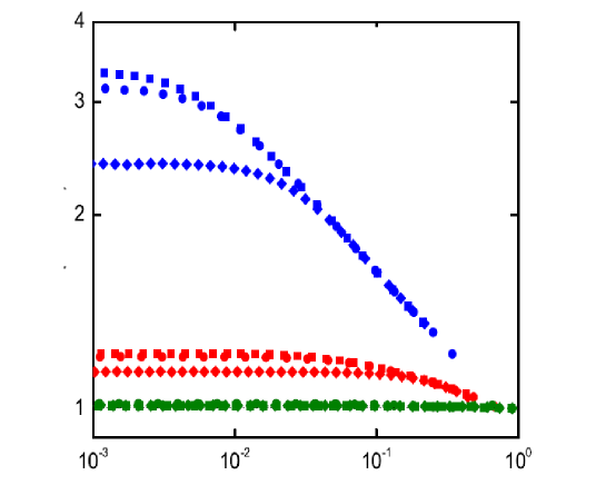
Figure 1: (color online) The correlation function Eq.(7) as a function of $\omega$ from direct diagonalization of the 3D Anderson model with critical disorder W=16.5 for disorder strength W=2 (green), W=5 (red) and W=10 (blue), and different system sizes L=8(diamond),L=16 (circles),L=20 (squares). At $W=10$ and $L=16,20$ the critical power-law is well seen for $(\nu_{0}\xi^{d})^{-1}=\delta_{\xi}<\omega<E_{0}$.

In Fig.1 it is shown the result of calculation of the correlation function Eq.(7) by direct diagonalization of the 3D Anderson model in the metallic phase with sub-critical disorder. One can see that even relatively far from the critical disorder ($W_{c}=16.5$), at $W=10$, the power-law critical behavior is well seen. It is saturated when the $\omega$-dependent ”resolution length” $L_{\omega}=(\nu_{0}\omega)^{-1/d}$ becomes larger than either the correlation length $\xi\propto(W_{c}-W)^{-\nu}$ or the system size $L$. Even at disorder as small as $W=5$ the enhancement of $M_{\omega}$ given by the factor $(E_{0}/\omega)^{\mu}$ in Eq.(7) is quite significant. Only at $W=2$ when $\xi<\ell=(\nu_{0}E_{0})^{\frac{1}{d}}$ it disappears, and we reach the limit $L^{d}M_{\omega}=1$ expected for the extended single particle wavefunctions which occupy all the available space.

Such a behavior of the correlation function Eq.(7) suggests a stricture of the typical single-particle wavefunction at the sub-critical disorder which is sketched in Fig.2.

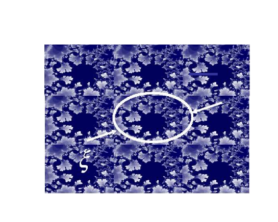
Figure 2: (color online) The cartoon of the amplitude landscape of the sub-critical single-particle wavefunction. The correlation length $\xi\propto(W_{c}-W)^{-\nu}$ sets the typical size of the ”fractal region” where the wavefunction correlations are the same as in the critical state. If the $\omega$-dependent ”resolution length” $L_{\omega}=(\nu_{0}\omega)^{-\frac{1}{d}}$ is smaller than $\xi$ the critical power law in Eq.(7) is well seen. For larger resolution length one observes a saturation in the $\omega$-dependence which is typical of metal. However, the fact that there are many peaks (dark regions on the plot)in the wavefunction landscape where the amplitude is pretty high, leads to the enhanced saturation level. The exception is the case of a very weak disorder when the correlation length $\xi\ll\ell$ is smaller than the size $\ell=(\nu_{0}E_{0})^{-\frac{1}{d}}$ of the ”pixel” which is only slightly larger than the atomic scale. Only in this limit the Anderson theorem may apply. The similar cartoon holds for the localized states at super-critical disorder. In this case the amplitude is exponentially small outside the localization radius $\xi$ but has the same fractal structure inside this radius. That allows to speak about the ”multifractal metal” and ”multifractal insulator” [8].

It consists of the ”fractal regions” of the size of the ”correlation radius” $\xi$ appearing in the scaling theory of localization. Inside such regions all the correlations are identical to those in the critical wavefunction. As the energy difference $\omega$ decreases the ”resolution length” $L_{\omega}=(\nu_{0}\omega)^{-\frac{1}{d}}$ increases and at $\omega<\delta_{\xi}=(\nu_{0}\xi^{d})^{-1}$ it exceeds the correlation length $\xi$. Only for such $\omega$ the correlation function Eq.(7) may show that the state is not critical but extended. Thus $\omega=\delta_{\xi}$ marks the onset of saturation in Fig.1 for $L\gg\xi$.

It is important that at large $\omega=E_{0}$ all curves in Fig.1 merge, in agreement with Eq.(7). This means that for $\omega<E_{0}$ the matrix element $M_{\omega}$ is enhanced compared to the ideal case of totally extended wavefunctions which occupy all the available space without peaks and holes at a scale much larger than the Fermi wavelength. In order to better understand the origin of this enhancement we emphasize that it is caused by the inhomogeneity of the amplitude $|\psi({\bf r})|^{2}$ in space. The presence of ”holes” with very small amplitude in certain regions implies appearance of peaks in other regions, as the integral of the amplitude over entire system of the size $L$ is equal to 1 by normalization. The key point is that the positions of the peaks in two different wave functions are highly correlated for the critical and slightly off-critical states. Contrary to naive expectation, even at large energy difference $\omega$ which is only slightly smaller than the upper energy scale for fractality $E_{0}$ (for the 3D Anderson model it is approximately 1/3 of the bandwidth), the correlation is pretty high. This leads to the very slow decay of the matrix element $M_{\omega}\sim\omega^{-\mu}$ ($\mu<1$) with increasing $\omega$ [10, 11]. Note that the ultimate reason for such a correlation is the presence of valleys in the random potential. All the wave functions are the solutions to the Schroedinger equation in the same random potential. So, the peaks know where they predominantly want to be situated. Yet, the criticality matters, as for localized states the similar correlation is absent, perhaps because there are too many possibilities to arrange a localized state of small localization radius. This is the reason why Eq.(7) can be formally extended to ideal metal by setting $d_{2}=d$ but it cannot be extended to hard insulator which formally corresponds to $d_{2}=0$.

3 The minimal model in real and in Fock space

As has been already mentioned in Introduction, in the situation when Coulomb interaction can be neglected the minimal model consists of the single-particle Hamiltonian with disorder and the local attractive interaction [12]:

$$\hat{H}=\sum_{{\bf r},{\bf r^{\prime}},\alpha}\varepsilon_{{\bf r},{\bf r^{\prime}}}\,\Psi^{{\dagger}}_{\alpha}({\bf r})\Psi_{\alpha}({\bf r^{\prime}})-U\sum_{{\bf r}}\Psi^{{\dagger}}_{\uparrow}({\bf r})\Psi^{{\dagger}}_{\downarrow}({\bf r})\Psi_{\downarrow}({\bf r})\Psi_{\uparrow}({\bf r}).$$ (9)

In the case where disorder is strong it is very useful to switch from the coordinate representation to the representation of the exact single-particle states where all effect of disorder is taken into account [13, 14]. This is done as usual by substitution $\Psi_{\alpha}({\bf r})=\sum_{n}\psi_{n}({\bf r})\,c_{n,\alpha}$ of the $\Psi$-operator in terms of the exact single-particle wavefunctions $\psi_{n}({\bf r})$ and the creation/annihilation operators $c^{{\dagger}}_{n,\alpha}$ and $c_{n,\alpha}$ of electrons in the corresponding state $n$ with the spin $\alpha$. As the result the single-particle part of the Hamiltonian becomes diagonal but the interaction part produces a variety of terms

$$\hat{H}=\sum_{n,\alpha}E_{n}\,c^{{\dagger}}_{n,\alpha}c_{n,\alpha}-U\sum_{n,k,m,l}\,M_{nkml}c^{{\dagger}}_{n,\uparrow}c^{{\dagger}}_{k,\downarrow}c_{m,\downarrow}c_{l,\uparrow},$$ (10)

where

$$M_{nkml}=\int d^{d}{\bf r}\,\psi^{*}_{n}({\bf r})\psi^{*}_{k}({\bf r})\psi_{m}({\bf r})\psi_{l}({\bf r}).$$ (11)

These terms may be divided into two major groups. The first one consists of the terms where all four indices are the same $n=k=m=l$ or there are two pairs of equal indices. The examples are $M_{n}\equiv M_{nnnn}$ and $M_{nm}\equiv M_{nnmm}$, as well as $\bar{M}_{nm}\equiv M_{nmmn}$. They do not change the parity of occupation of a single particle state but can only move a singlet pair from state $n$ to state $m$ ($M_{nnmm}$) or to flip the spin of the singly occupied state ($M_{nmnm}$). All the other terms may convert the singly-occupied state into the empty or doubly occupied states and vise versa.

In the region of localized single-particle states the largest matrix element is $M_{n}$, all the other matrix elements are smaller because different single-particle states rarely overlap. When the matrix element $-UM_{n}$ is large enough, it favors a local pair formation by producing a gap between the even many-body states in which all the single-particle states are occupied by a singlet pair or empty, and all other (odd) states. In this case one may neglect the presence of odd states whatsoever and introduce bosonic operators $b_{n}^{\dagger}=c^{\dagger}_{n\uparrow}c^{\dagger}_{n\downarrow}$. One can easily check that $(b^{\dagger}_{n})^{2}=0$, so that we introduced a hard-core bosons. In addition to that, for even states $b^{{\dagger}}_{n}b_{n}=c^{{\dagger}}_{n\uparrow}c_{n\uparrow}=c^{{\dagger}}_{n\downarrow}c_{n\downarrow}$.

The minimal model in the Fock space is obtained by neglecting of all terms except for those proportional to $M_{n}$ and $M_{nm}$. The corresponding Hamiltonian takes the form:

$$\hat{H}=\sum_{n}2E_{n}\,b^{{\dagger}}_{n}b_{n}-U\sum_{n,m}M_{nm}\,b^{{\dagger}}_{n}b_{m}+h.c.$$ (12)

It describes physics of local pairs with hard-core interaction attached to single-particle states $n$ with random energies $2E_{n}$ and hopping due to the attractive interaction of original electrons. The term proportional to $M_{n}$ is included into the chemical potential. Obviously, the hopping favors establishing a delocalized phase which at low enough temperature must be superfluid. Disorder, in contrast, is trying to localize the pairs.

Eq.(12) admits also a spin representation in which the hard-core nature of bosons is automatically included. To this end one introduces the spin-$1/2$ operators $S^{+}_{n}=b^{{\dagger}}_{n}=c^{\dagger}_{n\uparrow}c^{\dagger}_{n\downarrow}$ and $S^{z}_{n}=b^{{\dagger}}_{n}b_{n}-\frac{1}{2}=\frac{1}{2}\,[c^{{\dagger}}_{n\uparrow}c_{n\uparrow}+c^{{\dagger}}_{n\downarrow}c_{n\downarrow}-1]$. Then Eq.(12) takes the form:

$$\hat{H}=\sum_{n}2E_{n}\,S^{z}_{n}-U\sum_{n,m}M_{nm}\,S^{+}_{n}S^{-}_{m}+h.c.$$ (13)

In this language the Ising order corresponds to localized pairs and the $XY$ order corresponds to a superfluid phase.

So far we neglected the term proportional to $M_{nmmn}$ which is also operating in the even sector of the Hilbert space. It can be easily taken into account by adding the following term to the Hamiltonian:

$$-U\sum_{n,m}\bar{M}_{nm}\,S^{z}_{n}S^{z}_{m}=-U\sum_{n,m}\bar{M}_{nm}\,b^{{\dagger}}_{n}b_{n}b^{{\dagger}}_{m}b_{m}+UV^{-1}\sum_{n}b^{{\dagger}}_{n}b_{n}.$$ (14)

This term describes interaction (attraction) of bosons at different points in the Fock space. It favors phase separation with fixed pair occupation number $1$ or $0$ and thus disfavors establishing a coherent superfluid phase where the occupation number strongly fluctuates. This has an effect of reducing the superconducting/superfluid transition temperature. Such a suppression of $T_{c}$ by a factor of order 1 [16] does not change, however, the main conclusions of this paper.

Among other omitted terms the most significant are the following:

$$-U\sum_{n,m,l}M_{nnml}\,b^{{\dagger}}_{n}c_{m\downarrow}c_{l\uparrow}+h.c.$$ (15)

which describe dissociation and creation of pairs out of singly occupied single-particle states. They can be safely neglected in the region of sufficiently strongly localized single-particle states but have to be taken into account in the region of critical and sub-critical states where they determine the Ginzburg number ${\rm Gi}$.

4 Mean field approximation in the Fock space

The minimal model Eq.(13) is a good starting point not only in the region of localized single-particle states (the ”pseudo-gap” region) but also in the critical and sub-critical region, although in this case its derivation from the minimal model in real space Eq.(9) is not justified by a small parameter. Indeed, the standard mean-field treatment of the spin-model Eq.(13) yields the following equation for the critical temperature [15]:

$$\Delta_{E}=\frac{\lambda}{2}\int dE^{\prime}\,\Delta_{E^{\prime}}\,\frac{\tanh\left(\frac{E^{\prime}}{T}\right)}{E^{\prime}}\,M_{E-E^{\prime}},$$ (16)

where $M_{\omega}$ is given by Eq.(7) and $\lambda=U\nu_{0}$ is the dimensionless attraction constant.

At a weak disorder $M_{\omega}=1$ for $|\omega|<\omega_{D}$ and zero otherwise, and one can immediately recognize the standard BCS equation for $T_{c}$, albeit with $T$ instead of $2T$. This is the price of restriction to the odd sector of the Hilbert space. In case when there is no gap between the many-body states of the even and odd sectors, the latter is thermodynamically relevant even if dynamically both sectors are totally decoupled. We will show, however, that the accuracy of the mean-field approximation on the metallic side close to the Anderson localization transition is up to a constant pre-factor of order 1. With this uncertainty the difference by a factor of 2 discussed above is beyond the accuracy of the mean-field approach.

Let us apply the mean-field equation (16) to compute the $T_{c}$ in the critical region. Plugging Eq.(7) in Eq.(16) and making a rescaling $E\rightarrow T_{c}\,\varepsilon$, $E^{\prime}\rightarrow T_{c}\,\varepsilon^{\prime}$ one reduces the problem of $T_{c}$ to that of the eigenvalue $\bar{\lambda}^{-1}\equiv\lambda^{-1}\,(T_{c}/E_{0})^{\mu}\sim 1$ of the dimensionless linear integral operator. Then we immediately conclude that:

$$T_{c}\sim E_{0}\,\lambda^{\frac{1}{\mu}},\;\;\;\;\mu=1-\frac{d_{2}}{d}.$$ (17)

5 Ginzburg number and the accuracy of the mean-field approximation

As is well known, the thermodynamic fluctuations of phase and fluctuation of the local $T_{c}$ due to disorder restrict the region of validity of the mean-field approximation. To take into account correctly the first effect in the region of extended single-particle states one needs to include dissociation processes Eq.(15). Without such processes, for the minimum model in the Fock space Eq.(13), the mean-field approximation is exact in this region, as the matrix element $M_{nm}$ couples to an infinite number of states in the thermodynamic limit. When dissociation processes are properly accounted for [16] one arrives at a remarkable result:

$${\rm Gi}\equiv\frac{\Delta T_{c}}{T_{c}}\sim 1,$$ (18)

where $\Delta T_{c}$ is the ”fluctuation region”. The effects of multifractality cancel out in the ${\rm Gi}$ number, and it appears to be a universal number of order $1$ close to the Anderson localization transition [14].

In the region of sufficiently strongly localized single-particle states, the ${\rm Gi}$ number is mainly controlled by the effective coordination number $K$ of states coupled by the matrix element $M_{nm}$ in the minimal spin model Eq.(13). As one goes away from the Anderson transition, this number increases. One can show [16] that in this region:

$${\rm Gi}={\rm Gi_{1}}+\frac{{\rm Gi_{2}}}{K^{2}},$$ (19)

where ${\rm Gi_{1}}$ and ${\rm Gi_{2}}$ are universal numbers of order 1. This effect of decreasing of coordination number with increasing disorder invalidates the mean-field approximation at sufficiently strong disorder and finally leads to the superconductor to insulator transition.

Note however, that in the vicinity of the Anderson transition Eq.(18) holds true. Given the relationship between the Ginzburg number and the energy scale $J$ associated with the phase rigidity:

$$J=\frac{T_{c}^{(MF)}}{{\rm Gi}^{\frac{1}{3}}}$$ (20)

one concludes that the scale $J$ and the mean-field transition temperature $T_{c}^{(MF)}$ given by Eq.(17) differ by a universal factor of order 1. This implies that the phase fluctuations may reduce the true superconducting transition temperature by at most a universal factor of order 1 compared to the mean-field result Eq.(17).

6 Virial expansion method

In order to describe the behavior of transition temperature in the region of localized single-particle states where the mean-field approach breaks down, we exploit [16] the idea of virial expansion applied to the spin-model Eq.(13). To this end we analytically express the Cooper susceptibility $\chi_{C}(T)$ (the response of the spin $S^{+}$ to the infinitesimal perturbation $\Delta\,S^{+}$) as a sum of contributions of clusters of $M$ coupled spins:

$$\chi_{C}(T)=\sum_{M+1}^{\infty}\chi_{M}(T),$$ (21)

The true transition temperature corresponds to temperature $T_{c}$ when this series becomes divergent. According to D’Alembert criterion this happens when:

$$\lim_{M\rightarrow\infty}\frac{\chi_{M+1}(T_{c})}{\chi_{M}(T_{c})}=1.$$ (22)

In view of rapid increase of complexity of the analytical expressions for $\chi_{M}$ with increasing $M$, we truncated the series Eq.(21) and used the operative definition of $T_{c}$ in terms of small-cluster contributions $T_{c}^{(1)}$ and $T_{c}^{(2)}$:

$$\chi_{1}(T_{c}^{(1)})=\chi_{2}(T_{c}^{(1)}),\;\;\;\;\chi_{2}(T_{c}^{(2)})=\chi_{3}(T_{c}^{(2)}).$$ (23)

By evaluating $\chi_{1}$, $\chi_{2}$ and $\chi_{3}$ taking the energies $E_{n}$ and matrix elements $M_{nm}$ from exact diagonalization of the Anderson model on a 3D lattice and solving Eq.(23) numerically we were able to find statistics of $T_{c}^{(1)}$ and $T_{c}^{(2)}$ at different positions of Fermi level relative to the mobility edge. The average $T_{c}^{(1)}$ and $T_{c}^{(2)}$ appear to be in good agreement with each other which gave us a reasonable confidence in the convergence of the procedure.

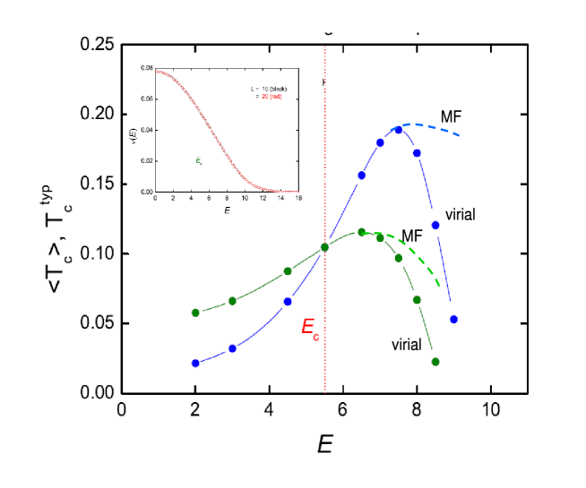
Figure 3: (color online)Transition temperature as a function of the Fermi energy position relative the mobility edge $E_{c}$ for the fixed dimensionless constant $\lambda=0.08$ (blue circles) and for the fixed attractive interaction $U=1.7t$(green circles), where $t$ is the hopping integral of the Anderson model. In the insert: energy dependence of the mean density of states. Large energy corresponds to region of localized single-particle states. Inside this region the mean-field (MF) transition temperature is substantially larger than that ($T_{c}\equiv\langle T_{c}^{(2)}\rangle$) found from the truncated virial expansion series. The Cooper susceptibilities $\chi_{2}(T)$ and $\chi_{3}(T)$ were calculated numerically using exact eigenfunctions and eigenvalues of the Anderson model with strength of disorder $W=4$, size of system $L=20^{3}$ and the Debye frequency $\omega_{0}=0.5$.

In Fig.3, the results of virial expansion calculation for the average $\langle T_{c}^{(2)}\rangle$ are presented as a function of the Fermi level position. It is remarkable that the truncated virial expansion method is in good agreement with the results of mean-field calculations in the region of extended and weakly localized states and gives substantially smaller transition temperature for stronger localized single-particle states. This proves that the virial expansion method, even with only 3 terms retained in the series Eq.(22), captures the decrease of the effective coordination number $K$ and is not equivalent to the mean-field approximation.

7 Enhancement of $T_{c}$ near the Anderson transition.

Equation (17) shows that when the Fermi energy is at the mobility edge $E=E_{c}$ the critical temperature behaves as a power law of the dimensionless attraction constant $\lambda$. Numerical simulations on the 3D Anderson model of localization give (see Ref. [16] and references therein) the value of the fractal dimension $d_{2}=1.29\pm 0.1$. Thus the exponent in the power law dependence of $T_{c}$ on $\lambda$ is close to $1/\mu\approx 1.8$. For small $\lambda$ one always has $\lambda^{1.8}\gg{\rm exp}(1/\lambda)$. In addition to that the characteristic energy $E_{0}$ is of electronic nature and it is typically higher than the Debye frequency $\omega_{0}$. Therefore we conclude that at small $\lambda$ the transition temperature given by Eq.(17) is much higher than the BCS transition temperature $T_{c}\sim\omega_{0}\,{\rm exp}(-1/\lambda)$. This enhancement of $T_{c}$ is also obtained by a virial expansion method which is completely independent of the mean-field approach. It can be easily traced back to the enhancement of the matrix element $M_{nm}$ shown in Fig.1.

In order to figure out how general is the effect of enhancement of $T_{c}$ at negligible Coulomb interaction, let us consider the case of weak multifractality $1-d_{2}/d\ll 1$. This case is relevant for the 2D metal [17, 18], where

$$1-\frac{d_{2}}{2}=\frac{1}{g},\;\;\;\;g=2\pi^{2}\nu_{0}D.$$ (24)

Expanding the matrix element $Eq.(\ref{Chalk})$ in the mean-field equation Eq.(16) up to the leading correction in $1/g$ $M_{\omega}\approx 1+\frac{1}{g}\,\ln(E_{0}/\omega)$ we obtain the $1/g$ correction to the transition temperature:

$$\frac{\delta T_{c}}{T_{c}}=\frac{1}{2g}\,\ln\left(\frac{\omega_{0}}{T_{c}}\right)\,\ln\left(\frac{E_{0}^{2}}{\omega_{0}T_{c}}\right)\sim\frac{1}{g}\,\ln^{2}\left(\frac{\omega_{0}}{T_{c}}\right).$$ (25)

We obtained the correction of the same order as in Ref.[4] given by Eq.(3) thus proving that our analysis at $\lambda\ll 1$ qualitatively applies also to the case of weak multifractality in 2D metals. Then Eq.(2) tells us that the really crucial assumption for enhancement of $T_{c}$ by disorder is the suppression of Coulomb interaction. Recently [19] this statement was confirmed by the RG analysis of the Finkelstein-like nonlinear sigma-model in $d=2$ and $d=2+\epsilon$ where only the short-range interactions were taken into account.

There are certain systems [20, 21] where one may suspect such a suppression. Moreover, the enhancement of $T_{c}$ just before the onset of the insulating behavior was observed in one of them with the dependence of $T_{c}$ on doping highly reminiscent of the Fig.3. More investigations are needed to confirm or reject this conjecture. In any case, the search for systems with suppressed Coulomb interaction (except for obvious case of cold neutral fermionic atoms with attractive interaction) is a challenging task which may open a door into a wonderful world without Coulomb interaction.

References

References

- [1] Anderson P W, 1959 J. Phys. Chem. Solids 11 26.
- [2] Abrikosov A A, Gor’kov L P, 1958 Zh. Eksp. Teor. Fiz. 35 1558; 1959 Zh. Eksp. Teor. Fiz. 38 319 [Sov. Phys. JETP 8, 1090 (1959); 9, 220 (1959)]; Abrikosov A A, Gor’kov L P, 1961 Zh. Eksp. Teor. Fiz. 39 1781 [Sov. Phys. JETP 12,1243 (1961)].
- [3] Finkelstein A M, 1987 Pis’ma ZhETF 45 37 [Sov.Phys.JETP Letters 45 46 (1987)]
- [4] Maekawa S, Fukuyama H, 1982 J.Phys.Soc.Jpn. 51 1380.
- [5] Wegner F, 1980 Z. Phys. B 36 209
- [6] Levitov L S, 1990 Phys.Rev.Lett. 64 547; Mirlin A D, Evers F, 2000 Phys.Rev.B 62 7920; Yevtushenko O, Kravtsov V E, 2003 J.Phys.A:Math.Gen. 36 8265; Yevtushenko O, Ossipov A, 2007 J.Phys.A: Math.Gen. 40 4691
- [7] Chalker J T, Daniel G J, 1988 Phys.Rev.Lett. 61 593; Chalker J T, 1990 Physica A 167 253
- [8] Kravstov V E, Cuevas E, 2007 Phys.Rev.B 76 235119
- [9] Kravstov V E, Ossipov A, Yevtushenko O M, 2010 Phys.Rev.B 82 161102
- [10] Kravtsov V E, Muttalib K A, 1997 Phys.Rev.Lett. 79 1913
- [11] Mirlin A D, Fyodorov V Y, 1997 Phys.Rev.B 55 16001
- [12] Ghosal A, Randeria M, Trivedi N, 2001 Phys.Rev.B 65 014501
- [13] Ma M, Lee P A, 1985 Phys.Rev.B 32 5658
- [14] Kapitulnik A, Kotliar G, 1985 Phys.Rev.Lett. 54 473; Kotliar G, Kapitulnik A, 1986 Phys.Rev.B 33 3146
- [15] Feigelman M V, Ioffe L B, Kravtsov V E, Yuzbashyan E A, 2007 Phys.Rev.Lett. 98 027001
- [16] Feigelman M V, Ioffe L B, Kravtsov V E, Cuevas E, 2010 Ann. Phys. 325 1368
- [17] Altshuler B L, Kravtsov V E, Lerner I V, 1986 JETP Letters 43 441
- [18] Efetov K B., Fal’ko V I, 1995 Europhys. Lett. 32 627
- [19] Burmistrov I S, Gornyi I V, Mirlin A D, 2011 arXiv:1102.3323.
- [20] Yamanaka S, 2010 J. Mater. Chem. 20 2922
- [21] Taguchi Y, Kitora A, Iwasa Y, 2006 Phys.Rev.Lett. 97 107001