Relating $\bf{B_{s}}$ Mixing and $\bm{B_{s}\to\mu^{+}\mu^{-}}$ with New Physics – An Update

Abstract

This document describes my talk (based on work by JoAnne Hewett, Sandip Pakvasa, Alexey Petrov, Gagik Yeghiyan and myself) given at the 2011 Meeting of the Division of Particles and Fields of the American Physical Society (8/9/11-8/13/11) hosted by the Physics Department at Brown University. We perform a study of the Standard Model (SM) fit to the mixing quantity $\Delta M_{B_{s}}$ in order to bound contributions of New Physics to $B_{s}$ mixing. We then use this to explore the branching fraction of $B_{s}\to\mu^{+}\mu^{-}$ in several models of New Physics (NP). In some cases, this constrains NP amplitudes for $B_{s}\to\mu^{+}\mu^{-}$ to lie below the SM component.

I Introduction

Here, I describe a calculation Golowich:2011cx carried out by JoAnne Hewett, Sandip Pakvasa, Alexey Petrov, Gagik Yeghiyan and myself (hereafter denoted collectively as GHPPY) in which we study the transition ${B_{s}\to\mu^{+}\mu^{-}}$ in the context of both the Standard Model (SM) and New Physics (NP). As described in Section 2, our approach involves the mixing mass difference $\Delta M_{B_{s}}$ as well. The ‘Update’ mentioned in the title refers to two items. The first is to apply to our analysis the LHC bound for the branching ratio ${\cal B}r_{B_{s}\to\mu^{+}\mu^{-}}$ which was recently made public by Ref. eps2011 . For example, this affects the exclusion region in parameter spaces of NP models (cf Figs. 3,5). The second update refers to a change in one of the inputs in the published article of Ref. Golowich:2011cx which modifies our determination of $\Delta M_{B_{s}}$ (cf Eq. (4)) and some other some of the numerical results displayed in this report. This is also taken into account in Version 2 of the arXiv listing of Ref. Golowich:2011cx .

Since this is a written version of a talk given at DPF 2011, I avoid theoretical complexities and limit the number of equations; these can be accessed in Ref. Golowich:2011cx . However, I will use this report to expand on the limited number of references shown in my DPF talk by including substantially more here.

Section 2 contains a summary of the current experimental situation regarding $B_{s}$ mixing and ${B_{s}\to\mu^{+}\mu^{-}}$ as well as SM predictions for ${\cal B}r_{B_{s}\to\mu^{+}\mu^{-}}$ and $\Delta M_{B_{s}}$. Most of the underlying theoretical formalism and derived relationships in this area are already well known. What is more important in comparing theory with current experiment is instead numerics, especially regarding the uncertainties encountered in SM predictions.

In Section 3, we describe how the comparison of $\Delta M_{B_{s}}^{\rm(SM)}$ with $\Delta M_{B_{s}}^{\rm(Expt)}$ yields phenomenological bounds on the NP $B_{s}$-mixing contribution $\Delta M_{B_{s}}^{\rm(NP)}$. This can, in turn, be used to constrain the magnitude of NP contributions to the $B_{s}\to\mu^{+}\mu^{-}$ decay mode. We implement this approach by exploring five possible NP models: an extra gauge boson $Z^{\prime}$, family symmetry, R-parity violating supersymmetry, a fourth sequential quark generation and flavor-changing Higgs models.

Our Summary appears in Section 4.

II Standard Model Analysis and Experimental Review

The numerical predictions we cite for ${\cal B}r_{B_{s}\to\mu^{+}\mu^{-}}^{\rm(SM)}$, $\Delta M_{B_{s}}^{\rm(SM)}$, etc are based in part upon inputs displayed in Table 1. These entries were the ones available when the analysis in Ref. Golowich:2011cx was being performed. Of course, improvements in such inputs over time will modify our results.

Table 1: Some Input Parameters

$\alpha_{s}(M_{Z})=0.1184\pm 0.0007$ Bethke:2009jm	$|V_{ts}|=0.0403^{+0.0011}_{-0.0007}$ PDG
$\Delta M_{B_{s}}=(117.0\pm 0.8)\times 10^{-13}~{}{\rm GeV}$ PDG	$\Delta\Gamma_{B_{s}}/\Gamma_{B_{s}}=0.092_{-0.054}^{+0.051}$ PDG
${\bar{m}}_{t}({\bar{m}}_{t})=(163.4\pm 1.2)~{}{\rm GeV}$ Melnikov:2000qh	$f_{B_{s}}\sqrt{{\hat{B}}_{B_{s}}}=275\pm 13$ MeV Laiho:2009eu
${\hat{B}}_{B_{s}}=1.33\pm 0.06$ Laiho:2009eu	$f_{B_{s}}=0.2388\pm 0.0095$ GeV Laiho:2009eu

In Table 1, the values for the Cabibbo-Kobayashi-Maskawa (CKM) matrix elements $|V_{ts}|$ and $|V_{tb}|$ are taken from the global fit of Eq. (11.27) in Ref. PDG . Another route to $|V_{ts}|$ results in the value given in Eq. (11.13) of Ref. PDG , $|V_{ts}|=0.0387\pm 0.0021$. In this instance, we have adopted the one in Table 1 because it has the smaller listed uncertainty. Finally, corresponding to the running mass ${\bar{m}}_{t}({\bar{m}}_{t})$ in Table 1 is the top quark pole mass $m_{t}^{\rm(pole)}=173.1\pm 1.3$.

II.1 About $\bm{B_{s}\to\mu^{+}\mu^{-}}$

Consider first the SM prediction for ${\cal B}r_{B_{s}\to\mu^{+}\mu^{-}}$. A direct calculation of this quantity in the SM gives

$${\cal B}r_{B_{s}\to\mu^{+}\mu^{-}}^{\rm(SM)}={1\over 8\pi^{5}}\cdot{M_{B_{s}}\over\Gamma_{B_{s}}}\cdot\left(G_{F}^{2}M_{W}^{2}m_{\mu}f_{B_{s}}|V_{\rm ts}^{*}V_{\rm tb}|\eta_{Y}Y({\bar{x}}_{t})\right)^{2}\left[1-4{m_{\mu}^{2}\over M_{B_{s}}^{2}}\right]^{1/2}\ \ ,$$

where $\eta_{Y}$ is a QCD factor, $Y({\bar{x}}_{t})$ is an Inami-Lin function Inami:1980fz and ${\bar{x}}_{t}\equiv{\bar{m}}_{t}^{2}({\bar{m}}_{t})/M_{W}^{2}$ where ${\bar{m}}_{t}$ is the running top-quark mass in ${\overline{{\rm MS}}}$ renormalization. As pointed out in Ref. Buras:2003td , inserting the SM expression for $\Delta M_{B_{s}}$ removes the $|V_{\rm ts}^{*}V_{\rm tb}|^{2}$ factor, thereby reducing the uncertainty in the SM branching ratio expression. It is this modified expression we use to obtain

$${\cal B}r_{B_{s}\to\mu^{+}\mu^{-}}^{\rm(SM)}={3\over 4\pi^{3}}\cdot{\Delta M_{B_{s}}^{\rm(Expt)}\over\Gamma_{B_{s}}}\cdot{(G_{F}M_{W}m_{\mu}\eta_{Y}Y)^{2}\over{\hat{\eta}}{\hat{B}}_{B_{s}}S_{0}({\bar{x}}_{t})}\left[1-4{m_{\mu}^{2}\over M_{B_{s}}^{2}}\right]^{1/2}=\left(3.3\pm 0.2\right)\times 10^{-9}\ \ ,$$ (1)

where the largest source of uncertainty arises from ${\hat{B}}_{B_{s}}$ followed by the dependence in $S_{0}({\bar{x}}_{t})$ (cf. discussion preceding Eq. (4)) on the $t$-quark mass.

In response to a request from a Session Organizer, my talk included a summary of the experimental situation for ${\cal B}r_{B_{s}\to\mu^{+}\mu^{-}}$. It has begun to change rather substantially. Below are values taken respectively from the Particle Data Group (PDG) PDG , the CDF collaboration Aaltonen:2011fi and a compilation (LHC) of LHCb and CMS data eps2011 , all in units of $10^{-9}$:

$${\cal B}r_{B_{s}\to\mu^{+}\mu^{-}}^{\rm(PDG)}<47\times 10^{-9}\qquad(\text{CL}\ =90\%)~{};\qquad{\cal B}r_{B_{s}\to\mu^{+}\mu^{-}}^{\rm(CDF)}=\left(18^{+11}_{-9}\right)\times 10^{-9}$$

$${\cal B}r_{B_{s}\to\mu^{+}\mu^{-}}^{\rm(LHC)}<9\times 10^{-9}\qquad(\text{CL}\ =90\%)~{};\qquad{\cal B}r_{B_{s}\to\mu^{+}\mu^{-}}^{\rm(LHC)}<11\times 10^{-9}\qquad(\text{CL}\ =95\%)\ \ .$$ (2)

The strongest bounds (from LHC), which have become publically available at the 2011 summer conferences, show just how rapidly data for the $B_{s}\to\mu^{+}\mu^{-}$ mode is being accumulated. The ‘NP Window’, currently

$${\cal B}r_{B_{s}\to\mu^{+}\mu^{-}}^{\rm(LHC)}/{\cal B}r_{B_{s}\to\mu^{+}\mu^{-}}^{\rm(SM)}\simeq 3.3\ \ ,$$

is expected to close sometime in 2012 if ${B_{s}\to\mu^{+}\mu^{-}}$ is not observed by then Bettler . As such, we are either getting near to encountering NP in this mode or testing the SM prediction. Either outcome is eagerly awaited.

II.2 About $\bm{\Delta M_{B_{s}}}$

The experimental value PDG for $\Delta M_{B_{s}}$,

$$\Delta M_{B_{s}}^{\rm(Expt)}=(117.0\pm 0.8)\times 10^{-13}~{}{\rm GeV}\ \ ,$$ (3)

is a very accurate one – the uncertainty amounts to about $0.7$%. The next-to-leading (NLO) SM formula is arrived at from an operator product expansion of the mixing hamiltonian Buras:1990fn ; Urban:1997gw . The short-distance dependence in the Wilson coefficient appears in the scale-insensitive combination $\eta_{B_{s}}S_{0}({\bar{x}}_{t})$, where the factor $S_{0}({\bar{x}}_{t})$ is another Inami-Lin function Inami:1980fz . Our determination yields $S_{0}({\bar{x}}_{t})=2.319\pm 0.028$. Also, we obtain $\eta_{B_{s}}=0.5525\pm 0.0007$ for the NLO QCD factor. From the numerical inputs discussed thus far, we find

$$\Delta M_{B_{s}}^{\rm(SM)}={\left(G_{\rm F}M_{\rm W}|V_{\rm ts}^{*}V_{\rm tb}|\right)^{2}\over 6\pi^{2}}M_{B_{s}}f^{2}_{B_{s}}{\hat{B}}_{B_{s}}\eta_{B_{s}}S_{0}({\bar{x}}_{t})=\left(125.2^{+13.8}_{-12.7}\right)\times 10^{-13}~{}{\rm GeV}$$ (4)

which is in accord with the experimental value of Eq. (3).

III New Physics Analysis

Let us first obtain a numerical (1$\sigma$) bound on the New Physics contribution to $\Delta M_{B_{s}}$. We then use this to constrain couplings in a variety of NP models and thereby learn something about the $B_{s}\to\mu^{+}\mu^{-}$ transition.

Accounting for NP as an additive contribution,

$$\Delta M_{B_{s}}^{\rm(Expt)}=\Delta M_{B_{s}}^{\rm(SM)}+\Delta M_{B_{s}}^{\rm(NP)}\ \ ,$$

we have from Eqs. (3),(4),

$$\Delta M_{B_{s}}^{\rm(NP)}=\left(-8.2^{+13.8}_{-12.7}\right)\times 10^{-13}~{}{\rm GeV}\ \ .$$

The error in $\Delta M_{s}^{\rm(expt)}$ has been included, but it is so small compared to the theoretical error in $\Delta M_{s}^{\rm(SM)}$ as to be negligible. The $1\sigma$ range for the NP contribution is thus

$$\Delta M_{B_{s}}^{\rm(NP)}=(-20.9\to+5.6)\times 10^{-13}~{}{\rm GeV}\ \ .$$

To proceed further without ambiguity, we would need to know the relative phase between the SM and NP components. Lacking this, we employ the absolute value of the largest possible number,

$$|\Delta M_{B_{s}}^{\rm(NP)}|\leq 20.9\times 10^{-13}~{}{\rm GeV}\ \ ,$$ (5)

to constrain the NP parameters.

Next is the issue of which model of NP to adopt. There are, in fact, a number of ways that NP can impact the SM:

• Extra gauge bosons (LR models, etc)

• Extra scalars (Multi-Higgs models, etc)

• Extra fermions (Little Higgs models, etc)

• Extra dimensions (Universal extra dimensions, etc)

• Extra global symmetries (Supersymmetry, etc)

For an analysis of $D^{0}$ mixing which includes as many as twenty-one NP models, see Ref. Golowich:2007ka . Here, however, we shall content ourselves with a smaller NP menu of five items. For each, we shall include a few, somewhat informal, introductory remarks.

Many NP models have multidimensional parameter spaces whose complexity hinders the ability to utilize the constraint of Eq. (5). Several strategies come to mind for addressing this situation. Our approach is possibly the simplest one – to employ whatever set of reasonable assumptions (and/or physical intuitions) which allow us to find paths in parameter space which relate $|\Delta M_{B_{s}}^{\rm(NP)}|$ to ${\cal B}r_{B_{s}\to\mu^{+}\mu^{-}}$. However, we plan to revisit this issue in future work.

III.1 Single Extra Vector Boson $\bm{Z^{\prime}}$

We should clarify what is meant by the title of this subsection. There are many $Z^{\prime}$ models, literally hundreds, which contain one or more of these hypothetical gauge bosons. What we have in mind is the subset of such models in which one $Z^{\prime}$ has a much lower mass than other NP degrees of freedom. This explains the ‘single’ extra vector boson $Z^{\prime}$. In this case, the NP contribution to $B_{s}$ mixing arises from the $Z^{\prime}$ pole diagram (cf Fig. 1). Moreover we assume that the $Z^{\prime}$ has SM couplings to lepton pairs, thus leaving us with two unknowns, the $Z^{\prime}$ mass $M_{Z^{\prime}}$ and the nondiagonal flavor coupling $g_{Z^{\prime}s{\bar{b}}}$.

Figure 1: $B_{s}$ Mixing via $Z^{\prime}$ exchange

The scaling with $Z^{\prime}$ parameters then goes as

$$\Delta M_{B_{s}}^{\rm(Z^{\prime})}\ \propto\ {g_{Z^{\prime}s{\bar{b}}}^{2}\over M_{Z^{\prime}}^{2}}\qquad\text{and}\qquad{\cal B}r_{B_{s}\to\mu^{+}\mu^{-}}^{\rm({Z^{\prime}})}\ \propto\ {g_{Z^{\prime}s{\bar{b}}}^{2}\over M_{Z^{\prime}}^{2}}\cdot{M_{Z}^{2}\over M_{Z^{\prime}}^{2}}\ \ ,$$

leading to

$${\cal B}r_{B_{s}\to\mu^{+}\mu^{-}}^{\rm({Z^{\prime}})}\leq 0.3\times 10^{-9}~{}\cdot\left({1~{}{\rm TeV}\over M_{Z^{\prime}}}\right)^{2}\ \ .$$

This value will lie below the corresponding SM prediction (${\cal B}r_{B_{s}\to\mu^{+}\mu^{-}}^{\rm(SM)}=3.3\times 10^{-9}$) even for a $Z^{\prime}$ mass as light as $M_{Z^{\prime}}>0.3$ TeV. So, this class of models will not dominate the SM result.

III.2 Family (‘Horizontal’) Symmetries

The motivation for Family Symmetries (FS) is to obtain an understanding (still needed!) of fermion masses and fermion mixing matrices. This subject has a relatively long history, first having been actively explored in the late 1970’s. However, it remains an area of theoretical interest up to recent times (e.g. see Ref. Lalak:2010bk where FCNC and CPV patterns are studied in the context of Family Symmetries).

Here is a brief overview, with details left for Ref. Golowich:2011cx . The gauge sector in the Standard Model has a large global symmetry which is broken by the Higgs interaction Sher:1988mj . By enlarging the Higgs sector, some subgroup of this symmetry can be imposed on the full SM lagrangian and the symmetry can be broken spontaneously. This family symmetry can be global fcnch as well as gauged Maehara:1977nq . If the new gauge couplings are very weak or the gauge boson masses are large, the difference between a gauged or global symmetry is rather difficult to distinguish in practice begmemor . In general there would be FCNC effects from both the gauge and scalar sectors. GHPPY analyze the gauge contribution. Consider the family gauge symmetry group $SU(3)_{G}$ acting on the three left-handed families. Spontaneous symmetry breaking will render all the gauge bosons massive. If the SU(3) is broken first to SU(2) before being completely broken, we may have an effective ‘low’ energy symmetry $SU(2)_{G}$. This means that the gauge bosons ${\bf G}\equiv\left\{G_{i}\right\}\ (i=1,\dots,3)$ have masses $m_{i}$ which are much lighter than those of the $\left\{G_{k}\right\}\ (k=4,\dots,8)$.

There is a history of applications of family symmetry in which the number of unknowns becomes reduced to manageable proportions. The whole story is rather involved, but the following gives an impression of some steps. As regards the gauge boson masses $\{m_{i}\}$, in a simple scheme of symmetry breaking Monich:1980rr one obtains $m_{1}=m_{3}$. There are in the family symmetry also four mixing matrices $U_{d},U_{u},U_{\ell}$, $U_{\nu}$, unknown except for the constraints

$$U_{u}^{\dagger}U_{d}=V_{\rm CKM}\qquad\text{and}\qquad U_{\nu}^{\dagger}U_{\ell}\ =V_{\rm MNSP}\ \ ,$$

where $V_{\rm CKM}$ and $V_{\rm MNSP}$ are respectively the well-known Cabibbo-Kobayashi-Maskawa and Maki-Nakagawa-Sakata-Pontcorvo mixing matrices for quarks and leptons. Through reasoning given in Refs. q7 , Harrison:2002er , it is somewhat possible to tame the zoo of unknown mixing parameters.

The upshot of all this is

$$\Delta M_{B_{s}}^{\rm(FS)}\ \propto\ {f^{2}\over m_{1}^{2}}\qquad\text{and}\qquad{\cal B}r_{B_{s}\to\mu^{+}\mu^{-}}^{\rm({FS})}\ \propto\ {f^{4}\over m_{1}^{4}}\ \ ,$$

where $f$ sets the scale of the interactions between the gauge-bosons and fermions. The above relations then yield the result

$${\cal B}r_{B_{s}\to\mu^{+}\mu^{-}}^{\rm({FS})}\leq 0.9\times 10^{-12}\ \ ,$$

which is tiny compared to the SM prediction.

III.3 R-parity Violating Supersymmetry

One of the models of New Physics that has a rich flavor phenomenology is R-parity violating (RPV) SUSY. R-parity distinguishes between particle and sparticle as

$$R_{P}=(-)^{3(B-L)+2S}=\left\{\begin{array}[]{ll}+1&\text{(particle)}\\ -1&\text{(sparticle)}\end{array}\right.$$

If R-parity is conserved and the initial state consists solely of ordinary matter, then intermediate and final states can contain only even numbers of sparticles. In this subsection, we lift this restriction by allowing the presence in the superpotential of terms

$${\cal W}_{\not R}=\frac{1}{2}\lambda_{ijk}L_{i}L_{j}E^{c}_{k}+\lambda_{ijk}^{\prime}L_{i}Q_{j}D^{c}_{k}+\frac{1}{2}\lambda_{ijk}^{\prime\prime}U_{i}^{c}D^{c}_{j}D^{c}_{k}$$

where $i=1,2,3$ are generation labels. We impose baryon number symmetry by setting $\lambda^{\prime\prime}$ to zero. Also, we will assume CP-conservation, so all couplings $\lambda_{ijk}$ and $\lambda_{ijk}^{\prime}$ become real-valued. The set of $\{\lambda_{ijk}\}$ occur for couplings to leptons whereas only the $\{\lambda_{ijk}^{\prime}\}$ occur in $B_{s}$ mixing. For example, the lagrangian describing RPV SUSY contributions to $B_{s}$ mixing can be written as

$${\cal L}_{\not R}=-\lambda_{i32}^{\prime}\widetilde{\nu}_{i_{R}}\overline{b}_{R}s_{L}-\lambda_{i23}^{\prime}\widetilde{\nu}_{i_{R}}\overline{s}_{R}b_{L}+h.c.\ \ ,$$

The crucial difference between studies of RPV SUSY contributions to phenomenology of the up-quark and down-type quark sectors is the possibility of tree-level diagrams contributing to $B_{s}$-mixing and $B_{s}\to\ell^{+}\ell^{-}$ decays Kundu:2004cv ; Kao:2009fg ; Dreiner:2006gu ; Saha:2002kt . Then a process like the one in Fig. 2 dominates. Note how the initial and final states consist of ordinary matter whereas the intermediate state has a single sneutrino – this is clearly $B_{s}$ mixing due to RPV dynamics.

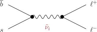
Figure 2: $B_{s}\to\ell^{+}\ell^{-}$ via sneutrino exchange

In RPV-SUSY, the underlying transition for $B_{s}\to\mu^{+}\mu^{-}$ is $s+{\bar{b}}\to\mu^{+}+\mu^{-}$ via tree-level $u$-squark or sneutrino exchange. In order to relate the rare decay to the mass difference contribution from RPV SUSY $\Delta M_{\rm B_{s}}^{\rm({\not R})}$, we need to assume that the up-squark contribution is negligible. This can be achieved in models where sneutrinos are much lighter than the up-type squarks, which are phenomenologically viable. Then it can be shown that the dependence of ${\cal B}r^{\rm({\not R})}_{B_{s}\to\mu^{+}\mu^{-}}$ on the RPV parameters becomes

$${\cal B}r^{\rm({\not R})}_{B_{s}\to\mu^{+}\mu^{-}}\ \propto\ \left(\frac{\lambda_{i22}\lambda_{i32}^{\prime}}{M_{\tilde{\nu}_{i}}^{2}}\right)^{2}\ \ .$$

Upon inserting the information from $\Delta M_{\rm B_{s}}^{\rm({\not R})}$ and assuming $\lambda_{k23}=\lambda_{k32}$, it is possible to plot the dependence of ${\cal B}r_{B_{s}\to\mu^{+}\mu^{-}}$ on $\lambda_{k22}$ for different values of $M_{\tilde{\nu}_{i}}$, which we present in Fig. 3.

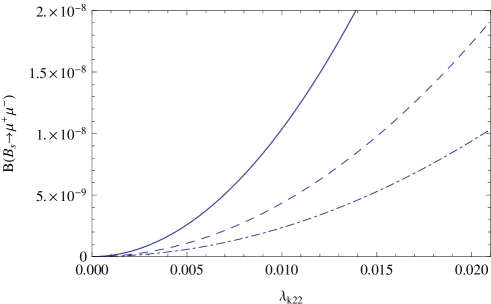
Figure 3: Branching ratio of ${\cal B}r_{B_{s}^{0}\to\mu^{+}\mu^{-}}$ as a function of RPV leptonic coupling $\lambda_{k22}$ and sneutrino mass $M_{\tilde{\nu}_{i}}=100$ GeV, $150$ GeV, and $200$ GeV (solid, dashed, and dash-dotted lines).

III.4 Fourth Quark Generation

One of the simplest extensions of the Standard Model involves addition of the sequential fourth generation (often denoted as SM4) of chiral quarks, $t^{\prime}$ and $b^{\prime}$ Holdom:2009rf ; Buras:2010pi ; Hou:2010mm . The addition of a sequential fourth generation of quarks leads to a 4$\times$4 CKM quark mixing matrix Chanowitz:2009mz . This implies that the parameterization of this matrix requires six real parameters and three phases. Besides providing new sources of CP-violation, the two additional phases can affect ${\cal B}r_{B_{s}\to\mu^{+}\mu^{-}}$ due to interference effects Bobrowski:2009ng .

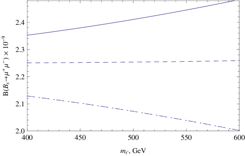
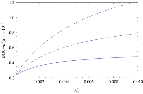
Figure 4: Left: branching ratio of ${\cal B}r_{B_{s}^{0}\to\mu^{+}\mu^{-}}$ as a function of the top-prime mass $m_{t^{\prime}}$ for different values of the phase $\phi_{t^{\prime}s}=0,\pi/2,\pi$ (solid, dashed, dash-dotted lines) and $\lambda_{bs}^{t^{\prime}}=|V_{t^{\prime}s}V_{t^{\prime}b}^{*}|\simeq 10^{-4}$ Alok:2010zj (see also Nandi:2010zx ). Right: branching ratio of ${\cal B}r_{B_{s}^{0}\to\mu^{+}\mu^{-}}$ as a function of the CKM parameter combination $\lambda_{bs}^{t^{\prime}}$ with $\phi_{t^{\prime}s}=0$ and different values of $m_{t^{\prime}}=400$ GeV (solid), $500$ GeV (dashed), and $600$ GeV (dash-dotted).

There are several existing constraints on the parameters related to the fourth generation of quarks, including direct searches, CKM unitarity tests, and fitting precision electroweak data (S and T parameters)  Novikov:1994zg ; Novikov:2001md ; Kribs:2007nz ; Erler:2010sk . The latter strongly constrains the masses of the new quarks. Finally, for the sake of completeness we take note of a data input which became available subsequent to our DPF 2011 talk – that null results in Higgs searches by the LHC detectors now place the scenario of a sequential fourth quark generation ‘in deep trouble’ lp2011 .

The relationship between $\Delta M_{B_{s}}$ and ${\cal B}r_{B_{s}\to\mu^{+}\mu^{-}}^{\rm(SM4)}$ has been previously studied in detail in Ref. Soni:2010xh . We shall update their result. In SM4, the branching ratio for $B_{s}\to\mu^{+}\mu^{-}$ can be related to the experimentally-measured $\Delta M_{B_{s}}^{\rm(Expt)}$ as Soni:2010xh

$${\cal B}r_{B_{s}\to\mu^{+}\mu^{-}}^{\rm(SM4)}\ \propto\ \Delta M_{B_{s}}^{\rm(Expt)}\frac{\left|C_{10}^{tot}\right|^{2}}{\left|\Delta^{\prime}\right|}\ \ ,$$

where the parameter $\Delta^{\prime}$ is a $B_{s}$-mixing loop parameter Soni:2010xh ,

$$\Delta^{\prime}=\eta_{t}S_{0}(x_{t})+\eta_{t^{\prime}}R_{t^{\prime}t}^{2}S_{0}(x_{t^{\prime}})+2\eta_{t^{\prime}}R_{t^{\prime}t}S_{0}(x_{t},x_{t^{\prime}})\ \ ,$$

$R_{t^{\prime}t}\equiv V_{t^{\prime}s}V_{t^{\prime}b}^{*}/V_{ts}V_{tb}^{*}$ and the definition of the function $S_{0}(x_{t},x_{t^{\prime}})$ can be found in Ref. Soni:2010xh . The Wilson coefficient $C_{10}^{tot}$ is defined as

$$C_{10}^{tot}(\mu)=C_{10}(\mu)+R_{t^{\prime}t}C_{10}^{t^{\prime}}(\mu)$$

with $C_{10}^{t^{\prime}}$ obtained by substituting $m_{t^{\prime}}$ into the SM expression for $C_{10}$ Buras:1994dj . Our results can be found in Fig. 4. Referring to the recent LHC bound of Eq. (2) on ${\cal B}r_{B_{s}\to\mu^{+}\mu^{-}}$, the exclusion regions on the ${B_{s}\to\mu^{+}\mu^{-}}$ branching ratio in Fig. 4 lies above $1.\times 10^{-8}$. As one can see, the resulting branching ratios are for the most part lower than the LHC experimental bound. However, with values of the CKM4 matrix element $\lambda_{bs}^{t^{\prime}}\equiv|V_{t^{\prime}s}V_{t^{\prime}b}^{*}|$ of about $0.01$, disfavored by Alok:2010zj , but still favored by Nandi:2010zx , ${\cal B}r_{B_{s}\to\mu^{+}\mu^{-}}^{\rm(SM4)}$ can still exceed the current bound.

III.5 Flavor-changing Neutral Current Higgs Bosons

Many extensions of the Standard Model contain multiple scalar doublets, which increase the possibility of FCNC mediated by flavor non-diagonal interactions of neutral components. While many ideas exist on how to suppress those interactions (see, e.g. Refs. Hall:1993ca ; Cheng:1987rs ; Pich:2009sp ), the ultimate test of those ideas would involve direct observation of scalar-mediated FCNC. The interest in multi-Higgs structures has remained fairly constant over the years and continues unabated to this day (e.g. see Ref. Buras:2010mh ).

A generic interaction hamiltonian of this type is

$${\cal H}^{H}=\frac{\phi^{0}}{\sqrt{2}}\left[\lambda_{23}^{D\dagger}\ \overline{b}_{R}s_{L}\ +\lambda_{32}^{D}\ \overline{b}_{L}s_{R}+\lambda_{22}^{E}\ \overline{\mu}_{L}\mu_{R}\right]-i\frac{a^{0}}{\sqrt{2}}\left[\lambda_{23}^{D\dagger}\ \overline{b}_{R}s_{L}\ +i\lambda_{32}^{D}\ \overline{b}_{L}s_{R}+\ i\lambda_{22}^{E}\ \overline{\mu}_{L}\mu_{R}\right]+\dots\ +\mbox{H.c.}\ \ ,$$

where $\phi^{0}$ and $a^{0}$ represent the lightest scalar and pseudoscalar states respectively and ellipses stand for the terms containing still heavier states whose contributions to $\Delta M_{B_{s}}$ and ${\cal B}r_{B_{s}\to\mu^{+}\mu^{-}}$ will be suppressed. We take all couplings $\lambda_{ij}^{D}$ and $\lambda_{ij}^{E}$ to be real-valued. The superscripts $D$ and $E$ on these refer respectively to couplings of $d$-type quarks and of charged leptons. To proceed, we need to distinguish two cases: the lightest FCNC Higgs particle as a scalar ($\phi^{0}$) or pseudoscalar ($a^{0}$).

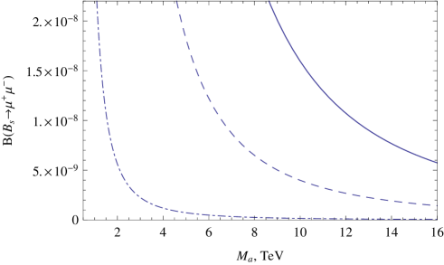
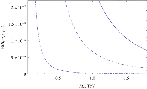
Figure 5: Branching ratio of ${\cal B}r_{B_{s}^{0}\to\mu^{+}\mu^{-}}$ as a function of pseudoscalar Higgs mass $M_{a}$. Left: $\lambda_{22}^{E}=1,0.5,0.1$ (solid, dashed, dash-dotted lines). Right: $\lambda_{22}^{E}=0.1,0.05,0.01$ (solid, dashed, dash-dotted lines).

III.5.1 Light scalar FCNC Higgs

The case of relatively light scalar Higgs state is quite common, arising most often in Type-III two-Higgs doublet models (models without natural flavor conservation) Barger:1989fj ; Atwood:1996vj ; Blechman:2010cs . Although the FCNC Higgs model does contribute to $\Delta M_{{\rm B}_{s}}$, it does not contribute to $B_{s}\to\mu^{+}\mu^{-}$ at tree level. Any nonzero contribution to $B_{s}\to\mu^{+}\mu^{-}$ decay must be produced at one-loop level Diaz:2004mk .

III.5.2 Light pseudoscalar FCNC Higgs

The case of a lightest pseudoscalar Higgs state can occur in the non-minimal supersymmetric standard model (NMSSM) Nilles:1982dy ; Ellis:1988er ; Ellwanger:1996gw ; Hiller:2004ii or related models Dobrescu:1999gv . In NMSSM, a singlet pseudoscalar is introduced to dynamically solve the $\mu$ problem. The resulting pseudoscalar can have a mass as light as tens of GeV. This does not mean, however, that it necessarily gives the dominant contribution to both $B_{s}$ mixing and the $B_{s}\to\mu^{+}\mu^{-}$ decay rate since there can be loop contributions from other Higgs states. However, here we work in the region of the parameter space where it does. Calculation reveals

$$\Delta M_{{\rm B}_{s}}^{\rm(a)}\ \propto\ \left({\lambda_{32}^{D}\over M_{a}}\right)^{2}\qquad\text{and}\qquad{\cal B}r_{B_{s}\to\ell^{+}\ell^{-}}^{\rm(a)}\ \propto\ \left({\lambda_{32}^{D}~{}\lambda_{22}^{E}\over M_{a}^{2}}\right)^{2}$$

In ${\cal B}r_{B_{s}\to\ell^{+}\ell^{-}}^{\rm(a)}$, the dependence on $\lambda_{32}^{D}$ can be eliminated by using $\Delta M_{{\rm B}_{s}}^{\rm(a)}$. The unknown factors then enter in the combination $\lambda_{22}^{E}/M_{a}$. In Fig. 5, we plot the dependence on $M_{a}$ for different values of $\lambda_{22}^{E}$.

IV Summary

Our talk consisted of two main parts, the (updated) SM evaluations of Ref. Golowich:2011cx and the issue of NP contributions to $B_{s}\to\mu^{+}\mu^{-}$. We discuss each of these in turn.

IV.1 Update of SM Evaluations

As regards $B_{s}$ mixing, we have

$$\Delta M_{B_{s}}^{\rm(Expt)}=(117.0\pm 0.8)\times 10^{-13}~{}{\rm GeV}\qquad\text{and}\qquad\Delta M_{B_{s}}^{\rm(SM)}=\left(125.2^{+13.8}_{-12.7}\right)\times 10^{-13}~{}{\rm GeV}\ \ .$$

The uncertainty in the SM result is seen to be about $16$ times larger than that in the experimental listing. It arises mainly from the factors $f^{2}_{B_{s}}{\hat{B}}_{B_{s}}$ and $|V_{\rm ts}|^{2}$ in Eq. (4) and is roughly equally shared between them. This large theoretical uncertainy in $\Delta M_{B_{s}}^{\rm(SM)}$ hinders the study of additive NP contributions.

As regards the $B_{s}\to\mu^{+}\mu^{-}$ branching ratio, upon using $\Delta M_{B_{s}}^{\rm(Expt)}$ as input (cf Eq. (1)), we obtain

$${\cal B}r_{B_{s}\to\mu^{+}\mu^{-}}^{\rm(SM)}=\left(3.3\pm 0.2\right)\times 10^{-9}\ \ .$$

We find the main uncertainty to be from ${\hat{B}}_{B_{s}}$ and roughly half as much from the implicit $t$-quark mass dependence in $S_{0}({\bar{x}}_{t})$.

IV.2 NP Contributions to $\bm{B_{s}\to\mu^{+}\mu^{-}}$

The GHPPY approach to $B_{s}\to\mu^{+}\mu^{-}$ is to use

$$\Delta M_{B_{s}}^{\rm(Expt)}=\Delta M_{B_{s}}^{\rm(SM)}+\Delta M_{B_{s}}^{\rm(NP)}$$

to bound $|\Delta M_{B_{s}}^{\rm(NP)}|$ and thus to constrain NP parameters. In this talk, I described the results of studying five NP models, with a sixth in preparaion. For two of them (the cases of a single $Z^{{}^{\prime}}$ and of family symmetry), we conclude that the contribution to $B_{s}\to\mu^{+}\mu^{-}$ lies below the SM prediction. For the others, Figs. 3-5 depict the regions of exclusion in their respective parameter spaces. We repeat our earlier comment that the exclusion regions in earlier versions Golowich:2011cx of our Figures are based on the PDG listing

$${\cal B}r_{B_{s}\to\mu^{+}\mu^{-}}^{\rm(PDG)}<47\times 10^{-9}\qquad(\text{CL}\ =90\%)$$

and have been updated here to reflect the combined LHCb and CMS bounds,

$${\cal B}r_{B_{s}\to\mu^{+}\mu^{-}}^{\rm(LHC)}<\ \left\{\begin{array}[]{ll}9\times 10^{-9}&\qquad(\text{CL}\ =90\%)\\ 11\times 10^{-9}&\qquad(\text{CL}\ =95\%)\ \ .\\ \end{array}\right.$$ (8)

As a final comment, we point out that the size of the SM contribution to $D^{0}\to\mu^{+}\mu^{-}$ Golowich:2009ii is quite feeble compared to that in $B_{s}\to\mu^{+}\mu^{-}$. It would appear that the $D^{0}\to\mu^{+}\mu^{-}$ decay mode could well be a fruitful arena to search for New Physics!

- (1) E. Golowich, J. Hewett, S. Pakvasa, A. Petrov, G. Yeghiyan, Phys. Rev. D83, 114017 (2011). [arXiv:1102.0009v2 [hep-ph]].
- (2) Guy Wilkinson, News from the Flavour Frontier – Heavy Quark Physics at the LHC, talk delivered at the International Europhysics Conference on High Energy Physics (Grenoble, France)
- (3) T. Inami and C.S. Lim, Prog. Theor. Phys. 65, 297 (1981) [Erratum-ibid. 65, 1772 (1981)].
- (4) A. J. Buras, Phys. Lett. B 566, 115 (2003) [arXiv:hep-ph/0303060].
- (5) A. J. Buras, M. V. Carlucci, S. Gori, G. Isidori, JHEP 1010, 009 (2010). [arXiv:1005.5310 [hep-ph]].
- (6) S. Bethke, Eur. Phys. J. C 64, 689 (2009) [arXiv:0908.1135 [hep-ph]].
- (7) K. Nakamura et al. [Particle Data Group Collaboration], J. Phys. G G37, 075021 (2010).
- (8) K. Melnikov and T. v. Ritbergen, Phys. Lett. B 482, 99 (2000) [arXiv:hep-ph/9912391].
- (9) J. Laiho, E. Lunghi and R. S. Van de Water, Phys. Rev. D 81, 034503 (2010) [arXiv:0910.2928 [hep-ph]].
- (10) T. Aaltonen et al. [ CDF Collaboration ], [arXiv:1107.2304 [hep-ex]].
- (11) Marc-Olivier Bettler, Search for at LHCb, talk delivered at DP 2011 (Providence, RI)
- (12) A. J. Buras, M. Jamin and P. H. Weisz, Nucl. Phys. B 347, 491 (1990).
- (13) J. Urban, F. Krauss, U. Jentschura and G. Soff, Nucl. Phys. B 523, 40 (1998) [arXiv:hep-ph/9710245].
- (14) E. Golowich, J. Hewett, S. Pakvasa and A. A. Petrov, Phys. Rev. D 76, 095009 (2007) [arXiv:0705.3650 [hep-ph]].
- (15) Z. Lalak, S. Pokorski, G. G. Ross, JHEP 1008, 129 (2010). [arXiv:1006.2375 [hep-ph]].
- (16) M. Sher, Phys. Rept. 179, 273 (1989).
- (17) S. Pakvasa and H. Sugawara, Phys. Lett. B 73, 61 (1978).
- (18) T. Maehara and T. Yanagida, Lett. Nuovo Cim. 19, 424 (1977); M. A. B. Beg and A. Sirlin, Phys. Rev. Lett. 38, 1113 (1977); C. L. Ong, Phys. Rev. D 19, 2738 (1979); F. Wilczek and A. Zee, Phys. Rev. Lett. 42, 421 (1979); A. Davidson, M. Koca and K. C. Wali, Phys. Rev. D 20, 1195 (1979), Phys. Rev. Lett. 43, 92 (1979).
- (19) S. Weinberg, UTTG-05-91, Proceedings High Energy Physics and Cosmology (Islamabad, Pakistan), M.A.B. Beg Memorial Volume.
- (20) V. A. Monich, B. V. Struminsky and G. G. Volkov, Phys. Lett. B 104, 382 (1981) [JETP Lett. 34, 213.1981 ZETFA,34,222 (1981 ZETFA,34,222-225.1981)].
- (21) J.D. Bjorken, S. Pakvasa and S.F. Tuan, Phys. Rev. D 66, 053008 (2002) [arXiv:hep-ph/0206116].
- (22) P. F. Harrison, D. H. Perkins and W. G. Scott, Phys. Lett. B 530, 167 (2002) [arXiv:hep-ph/0202074].
- (23) A. Kundu and J. P. Saha, Phys. Rev. D 70, 096002 (2004) [arXiv:hep-ph/0403154].
- (24) Y. Kao and T. Takeuchi, arXiv:0910.4980 [hep-ph].
- (25) H. K. Dreiner, M. Kramer and B. O’Leary, Phys. Rev. D 75, 114016 (2007) [arXiv:hep-ph/0612278].
- (26) J. P. Saha and A. Kundu, Phys. Rev. D 66, 054021 (2002) [arXiv:hep-ph/0205046]; we concur with a conclusion of Ref. Dreiner:2006gu regarding the missing factor of 4 in this paper.
- (27) B. Holdom, W. S. Hou, T. Hurth et al., PMC Phys. A3, 4 (2009) [arXiv:0904.4698 [hep-ph]].
- (28) A. J. Buras, B. Duling, T. Feldmann et al., JHEP 1009, 106 (2010) [arXiv:1002.2126 [hep-ph]].
- (29) W. -S. Hou, C. -Y. Ma, Phys. Rev. D82, 036002 (2010) [arXiv:1004.2186 [hep-ph]].
- (30) M. S. Chanowitz, Phys. Rev. D79, 113008 (2009) [arXiv:0904.3570 [hep-ph]].
- (31) M. Bobrowski, A. Lenz, J. Riedl and J. Rohrwild, Phys. Rev. D 79, 113006 (2009) [arXiv:0902.4883 [hep-ph]].
- (32) V. A. Novikov, L. B. Okun, A. N. Rozanov et al., Mod. Phys. Lett. A10, 1915-1922 (1995).
- (33) V. A. Novikov, L. B. Okun, A. N. Rozanov et al., Phys. Lett. B529, 111-116 (2002). [hep-ph/0111028].
- (34) J. Erler and P. Langacker, Phys. Rev. Lett. 105, 031801 (2010) [arXiv:1003.3211 [hep-ph]].
- (35) G. D. Kribs, T. Plehn, M. Spannowsky and T. M. P. Tait, Phys. Rev. D 76, 075016 (2007) [arXiv:0706.3718 [hep-ph]].
- (36) Michael Peskin, Summary of LP11 and Expectations for LP13, talk delivered at the XXV Iinternational Symposium on Lepton Photon Interactions at High Energies (Mumbai, India)
- (37) A. Soni, A. K. Alok, A. Giri, R. Mohanta and S. Nandi, Phys. Rev. D 82, 033009 (2010) [arXiv:1002.0595 [hep-ph]].
- (38) A. J. Buras, M. Munz, Phys. Rev. D52, 186-195 (1995). [hep-ph/9501281].
- (39) A. K. Alok, A. Dighe and D. London, arXiv:1011.2634 [hep-ph].
- (40) S. Nandi and A. Soni, arXiv:1011.6091 [hep-ph].
- (41) L. J. Hall and S. Weinberg, Phys. Rev. D 48, 979 (1993) [arXiv:hep-ph/9303241].
- (42) T. P. Cheng and M. Sher, Phys. Rev. D 35, 3484 (1987).
- (43) A. Pich and P. Tuzon, Phys. Rev. D 80, 091702 (2009) [arXiv:0908.1554 [hep-ph]].
- (44) V. D. Barger, J. L. Hewett and R. J. N. Phillips, Phys. Rev. D 41, 3421 (1990).
- (45) D. Atwood, L. Reina and A. Soni, Phys. Rev. D 55, 3156 (1997) [arXiv:hep-ph/9609279].
- (46) A. E. Blechman, A. A. Petrov and G. Yeghiyan, JHEP 1011, 075 (2010) [arXiv:1009.1612 [hep-ph]].
- (47) R. A. Diaz, R. Martinez and C. E. Sandoval, Eur. Phys. J. C 41, 305 (2005) [arXiv:hep-ph/0406265].
- (48) H. P. Nilles, M. Srednicki and D. Wyler, Phys. Lett. B 120, 346 (1983); J. M. Frere, D. R. T. Jones and S. Raby, Nucl. Phys. B 222, 11 (1983); J. P. Derendinger and C. A. Savoy, Nucl. Phys. B 237, 307 (1984).
- (49) J. R. Ellis, J. F. Gunion, H. E. Haber, L. Roszkowski and F. Zwirner, Phys. Rev. D 39, 844 (1989).
- (50) U. Ellwanger, M. Rausch de Traubenberg and C. A. Savoy, Nucl. Phys. B 492, 21 (1997) [arXiv:hep-ph/9611251].
- (51) G. Hiller, Phys. Rev. D 70, 034018 (2004) [arXiv:hep-ph/0404220].
- (52) B. A. Dobrescu, Phys. Rev. D 63, 015004 (2001) [arXiv:hep-ph/9908391].
- (53) E. Golowich, J. Hewett, S. Pakvasa and A. A. Petrov, Phys. Rev. D 79, 114030 (2009) [arXiv:0903.2830 [hep-ph]].