Micro helical polymeric structures produced by variable voltage direct electrospinning

S. P. Shariatpanahi^a, A. Iraji zad^∗a,b‡,I. Abdollahzadeh^a,R. Shirsavar^a,D. Bonn^c,d and R. Ejtehadi ^a

DOI:10.1039/C1SM06009K

Direct near field electrospinning is used to produce very long helical polystyrene microfibers in water. The pitch length of helices can be controlled by changing the applied voltage, allowing to produce both micro springs and microchannels. Using a novel high frequency variable voltage electrospinning method we found the helix formation speed and compared the experimental buckling frequency to theoretical expressions for viscous and elastic buckling. Finally we showed that the new method can be used to produce new periodic micro and nano structures.

Buckling of liquid or solid ropes, in which the falling rope on the surface forms a helical shape, has been investigated both theoretically and experimentally on stationary ^{1, 2, 3} and moving ^{4, 5, 6, 7}surfaces for typical length scales of centimetres to meters . Recently it was shown that using near field electrospinning ^{8, 9, 10, 11} the same buckling phenomenon can be used at very small length scales to produce micro helical structures. In these experiments an electrically charged liquid jet is accelerated using a high voltage potential directly along its axis toward a collector surface. Before the jet experiences any electrical instability^{12, 13} (as happens in usual electrospinning), it buckles and solidifies on the collector surface.

These fine structures can find many applications in technological fields like microelectronics, MEMS(Micro Electro Mechanical Systems), Microfluidics etc., but so far no detailed control over the fine structures has been possible. Kim et. al. used the method to directly electrospin polyethylene oxide (PEO) solutions; as the jet solidifies and buckles over a sharp electrode tip, hollow coiled cylindrical structures with lengths of a few micrometers were produced ⁹. Han et. al. showed that with the same process fine polystyrene helical fibers can be produced by using water as collector surface; the latter speeds up the solidification of the jet ⁸. Using the same method, here we show how the buckling process can be controlled so that a wide range of morphologies can be obtained: from straight fibers to helices and even micro channels. Furthermore for the first time we use a high frequency variable high voltage source that allows to control and measure the buckling frequency and the jet velocity. These measurements allow to compare the experimental results with existing theories for buckling.

Fig.1(a) shows the set up of the experiment; a high voltage potential difference is applied between the needle of a syringe and a bath of gently flowing water, $2.5cm$ apart. The straight jet of polymer solution coming out from a syringe needle is collected over the water surface and moves with the flow. The constant flow is made using a water container (the cylindrical container in the figure) with the high voltage electrode kept in the water close to the surface; the height of the water and consequently the flow velocity do not change considerably over the experiment time window.

As the polymer solution we used a Poly Styrene (PS) (Mw=350,000 a.m.u.) in Dimethyl Formamide(DMF); both from Sigma Aldrich. The solution solidifies rapidly as it touches the water so that after the process we obtain fine helical PS fibers. The process was controlled so that a long (up to tens of centimetres) buckled helical fiber is obtained (Fig.1(b,c)).

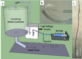
Fig.  1: (a) Schematic of the direct electrospinning experiment (b,c) long hollow coiled micro channels produced by direct electrospinning using water flow as collector

Collecting the fiber on a glass slide we could subsequently visualize it using optical microscopy. Figures 2 (a,b and c) show the helices produced for different polymer concentrations $C$ in constant applied voltage $V=4kV$. The most important observation that the fiber size can be controlled by changing the polymer concentration (table 1); the range we obtain here is from a few micrometers to a few hundreds of nanometers.

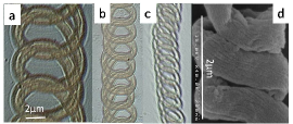
Fig.  2: Buckled helical structures: Optical microscope images with the same magnifications for: (a) $C=25wt\%,V=4kV$ (b) $C=15wt\%,V=4kV$ (c) $C=10wt\%,V=4kV$ and SEM image for (d) $C=10wt\%,V=6kV$

Table 1: Different fiber diameters for different solution concentrations $C$ (Fig 2)

$10wt\%$	$15wt\%$	$25wt\%$
$0.7\pm 0.1\mu m$	$1.1\pm 0.2\mu m$	$1.8\pm 0.2\mu m$

Fig.3 shows the helices for different applied voltages $V$ in constant concentration $C=25wt\%$. We find that the pitch length of the helices can be controlled with voltage from wide helices to channels formed by a dense helix. In addition we see that the fiber diameter remains almost constant as the voltage is varied. The pitch length can be measured for $3D$ structured helices taking into account the direction of observation. Fig.3(e) shows a schematic of a helix from its side view. An observer looking at an angle $\theta$ with the axis of the helix measures the radius of the helix $R$, the lengths $L_{1}$ and $L_{2}$. The pitch length $b$ of the helix is then easily found from:

$$L_{1}=\cos(\theta-\phi)\sqrt{(\frac{b}{2})^{2}+(2R)^{2}}$$

$$L_{2}=\sin(\theta)b$$

$$\tan(\phi)=\frac{b}{4R}$$ (1)

Table 2 shows the pitch lengths found for the different voltages.

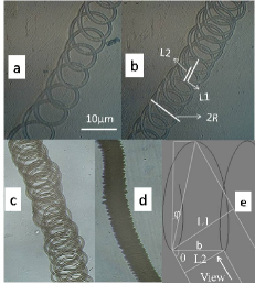
Fig.  3: Optical microscope images with the same magnifications of buckled helical fibers for: (a) $V=3kV,C=25wt\%$ (b) $V=4kV,C=25wt\%$ (c)$V=5kV,C=25wt\%$ (d)$V=6kV,C=25wt\%$ and (e) The helix geometry

Table 2: Different helix pitch lengths for different voltages $V$ (Fig 3)

$3kV$	$4kV$	$5kV$	$6kV$
$10\pm 1\mu m$	$5\pm 0.5\mu m$	$3.5\pm 0.5\mu m$	$1.5\pm 0.5\mu m$

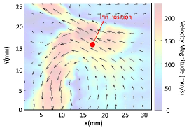
Fig.  4: Flow velocity field caused by ion wind over the water surface

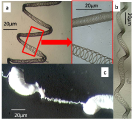
Fig.  5: Helical structure produced by applying a 3kV DC high voltage added to a sinusoidal 1.5 kV p-p variable voltage with frequencies (a) 200 Hz (b) 1 kHz using a $C=25wt\%$ solution. (c) New periodic structure produced by direct electrospinning using a square wave $5kV$ high voltage with frequency $100Hz$ .

Since we are clearly out of the range of electrical electrospinning instabilities ¹², it appears that the coiling we observe is purely mechanical. Recently, coiling instabilities have been studied in detail for both liquids and solids, and for both cases the coiling frequencies are well understood by now ¹⁴. To be able to confront our experiments to the theoretical predictions of Habibi et. al. ^{1, 2} we should determine the buckling frequency. In principle, this frequency can be deduced from the length scale of the coils and knowing the lateral velocity of advection of the buckled fiber⁸; however in our case the ion wind produced by the applied high voltage in air constitutes a problem ¹⁵. In the experiments, we observed a surface motion caused by the ion wind by recording the motion of added tracer particles smaller than $100\mu m$ with a high speed camera (Casio EX-F1). Using Particle Image Velocimetry (PIV) we subsequently measure their velocity at the surface of the water. As Fig.4 shows it is not possible here to measure the advection speed accurately, because the ion wind causes a complicated velocity field on the water surface. In addition the velocity of the flow is not necessarily the same as the velocity of the buckled fiber as it remains attached to the jet that falls from the orifice.

To be able to find the buckling frequency we used a novel method using a sinusoidal variation of the high voltage source superposed onto the DC voltage. As shown in Fig 5 the resulted buckled helices have variable pitch lengths and radius with the helix axis bended periodically in specific points. The variation of the pitch length and radius is due to the variable applied voltage during the fiber formation; while the bending of the helix, observed to occur after the buckling process, is caused by the variation of the spring constant along the helix axis. Since the bending points have the same axis length period as the pitch length variations we can consider these as the points with the same pitch length. In addition we observed the ion wind of the high frequency ($>100Hz$) voltage did not cause any flow on the water surface, so that the velocity of the water flow is constant while a considerable number of loops are formed. Since the velocity is constant, the axis length of the produced helix is proportional to time and we can safely assume that the length along the helix axis in each period is proportional to time the loops formed. So each photo works as a fast camera recording the buckling process and the buckling frequency is easily found by measurement of the pitch length. This allows to compare with the publications of Habibi et. al. ^{1, 2, 3}

To compare the experiments with the theory for buckling we introduce the following electrical $F_{e}$, inertial $F_{I}$, viscous $F_{\nu}$ and elastic $F_{E}$ forces per unit length to investigate the dynamics ^{9, 1, 2}. Then:

$$F_{e}\sim\epsilon_{0}e^{2}r$$

$$F_{I}\sim\frac{\rho r^{2}U^{2}}{R}$$

$$F_{\nu}\sim\frac{\rho\nu r^{4}U}{R^{4}}$$

$$F_{E}\sim\frac{Er^{4}}{R^{3}}$$ (2)

Where $r$ and $U$ are the radius and the velocity of the jet before buckling, $\rho$, $\nu$ and $E$ are the density, kinematic viscosity and the Young modulus of the jet, $R$ is the radius of the buckled helix, $\epsilon_{0}$ is the permeability of vacuum and $e$ is the electrical field. In our case the observed experimental parameters are of $U\sim 1m/s,r\sim 1\mu m,\rho\sim 10^{3}Kg/m^{3}$, $e\sim 10^{3}V/cm$ and $R\sim 10\mu m$ for which $F_{e}/F_{I}\sim 10^{-3}$. Habibi et. al. previously showed that for these conditions, the inertial forces are dominant: we are in the inertial regime of buckling. This result is different from previous work by Kim et. al. ⁹ in which the electrical forces in the focused field near the sharp electrode tip are much larger than the inertial forces. The question remains then whether the jet should be considered as a solid rope, or as a liquid filament. For these two different cases, the buckling frequency for the viscous ($\Omega_{I\nu}$) and elastic jets ($\Omega_{IE}$) are given by ^{1, 2}.:

$$\Omega_{I\nu}=\frac{1}{2\pi}(\frac{(\pi U)^{4}}{\nu r^{2}})^{1/3}$$

$$\Omega_{IE}=\frac{1}{2\pi}U^{2}(\frac{\rho}{d^{2}E})^{1/2}$$ (3)

In which $d=2r$ is the diameter of the fiber. Although these results are for buckling on a surface that does not move, it can be shown that the lateral motion of the surface does not affect the results significantly ⁶. Since during the experiment the viscous PS solution changes to a solid elastic material rapidly when it touches the water, to find out what the proper model for the buckling is we have to measure both the viscosity of the jet before the buckling and the Young’s modulus after this happens. The kinematic viscosity of the solution was determined using a Physica MCR301 rheometer to be $5000cm^{2}s^{-1}$. For the Young’s modulus measurement we found the spring constant of the buckled helix using a needle for stretching the helical structure over a precision balance(Fig 6). The helical fibers showed elastic behaviour for strains smaller than $25\%$ which was sufficient for an accurate measurement of the spring constant. Measuring the spring pitch length, helix radius and fiber diameter, we find the Young’s modulus to be almost $E=4GPa$, very similar to the usual bulk PS material ($3.5GPa$).

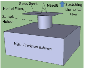
Fig.  6: Schematic of the experiment for measuring the spring constant of the helical fibers using a needle for stretching the helical structure over a precision balance

These measurements allow us to confront the experimental results to the predictions for viscous and elastic coiling. Fig7 shows the buckling frequency vs $U^{2}/d$ on a log-log scale. The elastic model predicts a slope of unity, whereas for viscous coiling the slope would be $2/3$ (see Eqn. 3). For the experimental data, the slope of we find is always smaller than but comparable to $2/3$ which suggests that the buckling is more viscous than elastic in character. More quantitatively, Fig 7 shows that the viscous model somewhat overestimates most of the experimentally measured frequencies. This can in fact be explained by assuming that the viscosity during the buckling is a little higher than the bulk one measured in the rheometer. This difference may be due to the thin ($\sim 1\mu m$ diameter) jet starting to solidify because of solvent evaporation. The importance of evaporation in these type of experiments is also reported by other groups ^{9, 10}.

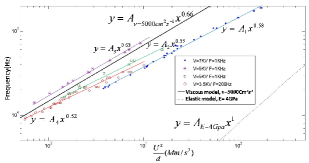
Fig.  7: Comparison between the theoretical models ^{1, 2} and the experimental results for different DC voltages $V$ and different variable $1.5kVP-P$ voltage frequencies $F$

As a bonus, the method employed here also allows to manufacture different types of periodic structures. As an example Fig 5 (c) shows such a structure made by applying square wave high voltage with $100Hz$ frequency and $5kV$ p-p amplitude. The structure consists of many hollow cavities connected periodically to each other. The cavities are produced by buckling and parallel fibers can be easily observable on their body. Since the parameter range in these experiments is rather large, one may find a large number of novel structures; however this is beyond the scope of the current paper.

In conclusion, we used a direct electrospinning method to produce buckled helical PS fibers with controlled pitch lengths. We used a high variable sinusoidal voltage added to the usual electrospinning high DC voltage to measure the experimental buckling frequency which showed a better agreement with the theoretical viscous rope buckling model than with the elastic one. Finally we introduced the new electrospinning technique as a method to produced new fine periodic micro structures whose characteristics can be controlled by experimental parameters such as the polymer concentration or the applied voltage.

References

- Habibi et al. 2010 M. Habibi, Y. Rahmani, D. Bonn and N. M. Ribe, Phys. Rev. Lett., 2010, 104, 074301.
- Maleki et al. 2004 M. Maleki, M.Habibi, R. Golestanian, N. M. Ribe and D. Bonn, Phys. Rev. Lett., 2004, 93, 214502.
- Habibi et al. 2007 M. Habibi, N. M. Ribe and D. Bonn, Phys. Rev. Lett., 2007, 99, 154302.
- Bergou et al. 2010 M. Bergou, B. Audoly, E. Vouga, M. Wardetzky and E. Grispun, ACM Transactions on Graphics, 2010, 29, doi:10.1145/1778765.1778853.
- Morris et al. 2008 W. Morris, J. H. P. Dawes, N. M. Ribe and J. R. Lister, Phys. Rev. E, 2008, 77, 066218.
- Ribe et al. 2006 N. M. Ribe, J. R. Lister and S. Chiu-Webster, Phys. Fluids., 2006, 18, 124105.
- Chiu-Webster and Lister 2006 S. Chiu-Webster and J. R. Lister, J. Fluid. Mech., 2006, 569, 89.
- Han et al. 2007 T. Han, D. H. Reneker and A. L. Yarin;, Polymer, 2007, 48, 6064.
- Kim et al. 2010 H. Y. Kim, M. Lee, K. J. P. S. Kim and M.Mahadevan, Nano. Lett., 2010, 10, 2138.
- Wang et al. 2010 H. Wang, G. Zheng, W. Li, X. Wang and D. Sun, Appl. Phys. A, 2010, 102, 457.
- Yu et al. 2008 J. Yu, Y. Qiu, X. Zha, M. Yu, J. Yu, J. Rafique and J. Yin, European. Polymer. Journal, 2008, 44, 2838.
- Reneker et al. 2000 D. H. Reneker, A. L. Yarin, H. Fong and S. Koombhongse, J. Appl. Phys., 2000, 87, 4531.
- Yarin et al. 2001 A. L. Yarin, S. Koombhongse and D. H. Reneker, J. Appl. Phys., 2001, 89, 3018.
- Ribe et al. to be published N. M. Ribe, M. Habibi and D. Bonn, Ann. Rev. Fluid., to be published.
- Kawamoto and Umezu 2005 H. Kawamoto and S. Umezu, J. Phys. D: Appl. Phys., 2005, 38, 887.