Tamari lattices and parking functions:
proof of a conjecture of F. Bergeron

Abstract.

An $m$-ballot path of size $n$ is a path on the square grid consisting of north and east unit steps, starting at $(0,0)$, ending at $(mn,n)$, and never going below the line $\{x=my\}$. The set of these paths can be equipped with a lattice structure, called the $m$-Tamari lattice and denoted by $\mathcal{T}_{n}^{(m)}$, which generalizes the usual Tamari lattice $\mathcal{T}_{n}$ obtained when $m=1$. This lattice was introduced by F. Bergeron in connection with the study of coinvariant spaces. He conjectured several intriguing formulas dealing with the enumeration of intervals in this lattice. One of them states that the number of intervals in $\mathcal{T}_{n}^{(m)}$ is

$$\frac{m+1}{n(mn+1)}{(m+1)^{2}n+m\choose n-1}.$$

This conjecture was proved recently, but in a non-bijective way, while its form strongly suggests a connection with plane trees.

Here, we prove another conjecture of Bergeron, which deals with the number of labelled intervals. An interval $[P,Q]$ of $\mathcal{T}_{n}^{(m)}$ is labelled if the north steps of $Q$ are labelled from 1 to $n$ in such a way the labels increase along any sequence of consecutive north steps. We prove that the number of labelled intervals in $\mathcal{T}_{n}^{(m)}$ is

$${(m+1)^{n}(mn+1)^{n-2}}.$$

The form of these numbers suggests a connection with parking functions, but our proof is non-bijective. It is based on a recursive description of intervals, which translates into a functional equation satisfied by the associated generating function. This equation involves a derivative and a divided difference, taken with respect to two additional variables. Solving this equation is the hardest part of the paper.

Finding a bijective proof remains an open problem.

1. Introduction and main results

An $m$-ballot path of size $n$ is a path on the square grid consisting of north and east unit steps, starting at $(0,0)$, ending at $(mn,n)$, and never going below the line $\{x=my\}$. It is well-known that there are

$$\frac{1}{mn+1}{(m+1)n\choose n}$$

such paths [6], and that they are in bijection with $(m+1)$-ary trees with $n$ inner nodes. Bergeron recently defined on the set $\mathcal{T}_{n}^{(m)}$ of $m$-ballot paths of size $n$ a partial order. It is convenient to describe it via the associated covering relation, exemplified in Figure 1.

Definition 1.

Let $P$ and $Q$ be two $m$-ballot paths of size $n$. Then $Q$ covers $P$ if there exists in $P$ an east step $a$, followed by a north step $b$, such that $Q$ is obtained from $P$ by swapping $a$ and $S$, where $S$ is the shortest factor of $P$ that begins with $b$ and is a (translated) $m$-ballot path.

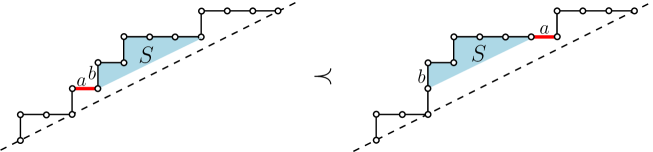
Figure 1. The covering relation between $m$-ballot paths ($m=2$).

It was shown in [4] that this order endows $\mathcal{T}_{n}^{(m)}$ with a lattice structure, which is called the $m$-Tamari lattice of size $n$. When $m=1$, it coincides with the classical Tamari lattice [2, 7, 15, 16]. Figure 2 shows two of the lattices $\mathcal{T}_{n}^{(m)}$.

Figure 2. The $m$-Tamari lattice $\mathcal{T}_{n}^{(m)}$ for $m=1$ and $n=4$ (left) and for $m=2$ and $n=3$ (right). The three walks surrounded by a line in $\mathcal{T}_{4}^{(1)}$ form a lattice that is isomorphic to $\mathcal{T}_{2}^{(2)}$ (see Proposition 4).

These lattices are conjectured to have deep connections with the ring $\operatorname{DR}_{3,n}$ of polynomials in three sets of variables $X=\{x_{1},\ldots,x_{n}\}$, $Y=\{y_{1},\ldots,y_{n}\}$, $Z=\{z_{1},\ldots,z_{n}\}$, quotiented by the ideal generated by (trivariate) diagonal invariants. By diagonal invariants, one means constant term free polynomials that are invariant under the following action of the symmetric group ${\mathfrak{S}}_{n}$: for $\sigma\in{\mathfrak{S}}_{n}$ and $f$ a polynomial,

$$\sigma(f(X,Y,Z))=f(x_{\sigma(1)},\ldots,x_{\sigma(n)},y_{\sigma(1)},\ldots,y_{\sigma(n)},z_{\sigma(1)},\ldots,z_{\sigma(n)}).$$

We refer to [1, 4] for details about these conjectures, which have striking analogies with the much studied case of two sets of variables [10, 11, 13, 14, 17]. In particular, it seems that the role played by ballot paths for two sets of variables (see, e.g., [8, 9, 12]) is played for three sets of variables by intervals of ballot paths in the Tamari order.

For instance, it is conjectured in [1] that the the dimension of a certain polynomial ring related to $\operatorname{DR}_{3,n}$, but involving one more parameter $m$, is

$$\frac{m+1}{n(mn+1)}{(m+1)^{2}n+m\choose n-1},$$ (1)

and that this number counts intervals in the Tamari lattice $\mathcal{T}_{n}^{(m)}$ . The latter statement was proved in [4] (the special case $m=1$ had been proved earlier [5]). The former one is presumably extremely difficult, given the complexity of the corresponding result for two sets of variables [13]. The dimension related result was observed earlier for small values of $n$ by Haiman [14] in the case $m=1$.

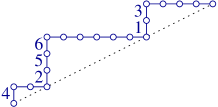
Figure 3. A labelled $2$-ballot path.

The aim of this paper is to prove another conjecture of [1], dealing with labelled Tamari intervals. Let us say that an $m$-ballot path of size $n$ is labelled if the north steps are labelled from 1 to $n$, in such a way the labels increase along any sequence of consecutive north steps (Figure 3). The number of labelled $m$-ballot paths of size $n$ is

$$(mn+1)^{n-1}.$$

Indeed, these paths are in bijection with $(1,m,\ldots,m)$-parking functions of size $n$, in the sense of [19, 20]: the function $f$ associated with a path $Q$ satisfies $f(i)=k$ if the north step of $Q$ labelled $i$ lies at abscissa $k-1$. Now, we say that an $m$-Tamari interval $[P,Q]$ is labelled, if the upper path $Q$ is labelled. It is conjectured in [1] that the number of labelled $m$-Tamari intervals of size $n$ is

$${(m+1)^{n}(mn+1)^{n-2}},$$ (2)

and this is what we prove in this paper. It is also conjectured in [1] that this number is the dimension of a certain polynomial ring generalizing $\operatorname{DR}_{3,n}$ (which corresponds to the case $m=1$).

Our proof is, at first blush, analogous to the proof of (1) presented in [4]: we introduce a generating function $F^{(m)}(t;x,y)$ counting labelled intervals according to three parameters; we describe a recursive construction of intervals and translate it into a functional equation defining $F^{(m)}(t;x,y)$ ; we finally solve this equation, after having partially guessed its solution. However, the labelled case turns out to be significantly more difficult than the unlabelled one. It is not hard to explain the origin of this increased difficulty: for $m$ fixed, the generating function of the numbers (1) is an algebraic series, and can be expressed in terms of the series $Z\equiv Z(t)$ satisfying

$$Z=\frac{t}{(1-Z)^{m(m+2)}}.$$

There exists a wealth of tools, both modern or ancient, to handle algebraic series (e.g., factorisation, elimination, Gröbner bases, rational parametrizations when the genus is zero, efficient guessing techniques, all tools made effective in Maple and its packages, like algcurves and gfun). Such tools play a key role in the proof of (1). But the generating function of the numbers (2) is related to the series $Z$ satisfying

$$Z=te^{m(m+1)Z},$$

which lives in the far less polished world of differentially algebraic series, for which much fewer tools are available.

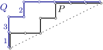
Figure 4. A labelled $2$-Tamari interval $I=[P,Q]$ of size $|I|=3$. It has $c(P)=3$ contacts, and its initial rise is $r(Q)=2$.

Our main result is actually more general that (2). Indeed, we refine the enumeration by taking into account two more parameters, which we now define. A contact of an $m$-ballot path $P$ is a vertex of $P$ lying on the line $\{x=my\}$. The initial rise of a ballot path $Q$ is the length of the initial run of up steps in $Q$. A contact of a Tamari interval $[P,Q]$ is a contact of the lower path $P$, while the initial rise of this interval is the initial rise of the upper path $Q$ (see Figure 4). We consider the exponential generating function of labelled $m$-Tamari intervals, counted by the size, the number of contacts and the initial rise. More precisely,

$$F^{(m)}(t;x,y)=\sum_{I=[P,Q]}\frac{t^{|I|}}{|I|!}\,x^{c(P)}y^{r(Q)},$$ (3)

where the sum runs over all labelled $m$-Tamari intervals $I$, $|I|$ denotes the size of $I$ (that is, the number of up steps in $P$), $c(P)$ the number of contacts of $P$ and $r(Q)$ the initial rise of $Q$. The main result of this paper is a complicated closed form expression of $F^{(m)}(t;x,y)$, which becomes simple when $y=1$. In particular, extracting the $n^{\hbox{th}}$ coefficient in $F^{(m)}(t;1,1)$ proves Bergeron’s conjecture (2).

Theorem 2.

Let $F^{(m)}(t;x,y)\equiv F(t;x,y)$ be the exponential generating function of labelled $m$-Tamari intervals, defined by (3). Let $z$ and $u$ be two indeterminates, and write

$$t=ze^{-m(m+1)z}\quad\hbox{and }\quad x=({1+u})e^{-mzu}.$$ (4)

Then $F(t;x,1)$ becomes a series in $z$ with polynomial coefficients in $u$, and this series has a simple expression:

$$F(t;x,1)=(1+u)e^{(m+1)z-(m-1)zu}\left(1+\frac{1-e^{mzu}}{u}\right).$$ (5)

In particular,

$$F(t;1,1)=(1-mz)e^{(m+1)z},$$

and the number of labelled $m$-Tamari intervals of size $n$ is

$$n![t^{n}]F(t;1,1)={(m+1)^{n}(mn+1)^{n-2}}.$$

Our expression of $F^{(m)}(t;x,y)$ is given in Theorem 17. When $m=1$, it takes a reasonably simple form, which we now present (the case $m=2$ is also detailed at the end of the paper). Given a Laurent polynomial $P(u)$ in $u$, we denote by $[u^{\geq}]P(u)$ the non-negative part of $P(u)$ in $u$, defined by

$$[u^{\geq}]P(u)=\sum_{i\geq 0}P_{i}u^{i}\quad\hbox{ if }\quad P(u)=\sum_{i\in{\mathbb{Z}}}P_{i}u^{i}.$$

The definition is then extended by linearity to power series whose coefficients are Laurent polynomials in $u$.

Theorem 3.

Let $F^{(1)}(t;x,y)\equiv F(t;x,y)$ be the generating function of labelled $1$-Tamari intervals, defined by (3). Let $z$ and $u$ be two indeterminates, and set

$$t=ze^{-2z}\quad\hbox{and }\quad x=({1+u})e^{-zu}.$$ (6)

Then $F(t;x,y)$ becomes a formal power series in $z$ with polynomial coefficients in $u$ and $y$, which is given by

$$F(t;x,y)=(1+u)\,e^{2yz}\ [u^{\geq}]\Big{(}e^{zu(y-1)+zy\bar{u}}-\bar{u}e^{z\bar{u}(y-1)+zyu}\Big{)},$$ (7)

with $\bar{u}=1/u$. Equivalently,

$$\frac{F(t;x,y)}{(1+u)e^{2yz}}=\sum_{0\leq i\leq j}u^{j-i}\frac{z^{i+j}y^{i}(y-1)^{j}}{i!j!}-\sum_{0\leq j<i}u^{i-j-1}\frac{z^{i+j}y^{i}(y-1)^{j}}{i!j!}.$$

It is easily seen that the case $y=1$ of the above formula reduces to the case $m=1$ of (5). When $x=1$, that is, $u=0$, the double sums in the expression of $F(t;x,y)$ reduce to simple sums, and the generating function of labelled Tamari intervals is expressed in terms of Bessel functions:

$$\frac{F(t;1,y)}{e^{2yz}}=\sum_{i\geq 0}\frac{z^{2i}y^{i}(y-1)^{i}}{i!^{2}}-\sum_{j\geq 0}\frac{z^{2j+1}y^{j+1}(y-1)^{j}}{(j+1)!j!}.$$

The outline of the paper goes as follows: in Section 2 we derive from a recursive description of labelled Tamari intervals a functional equation satisfied by their generating function. This equation involves a derivative (with respect to $y$) and a divided difference (with respect to $x$). We present in Section 3 the principle of the proof, and exemplify it on the case $m=1$, thus obtaining Theorem 3 above. Section 4 deals with the general case, and proves Theorem 2.

We conclude this introduction with some notation and a few definitions. Let $\mathbb{K}$ be a commutative ring and $t$ an indeterminate. We denote by $\mathbb{K}[t]$ (resp. $\mathbb{K}[[t]]$) the ring of polynomials (resp. formal power series) in $t$ with coefficients in $\mathbb{K}$. If $\mathbb{K}$ is a field, then $\mathbb{K}(t)$ denotes the field of rational functions in $t$, and $\mathbb{K}((t))$ the field of Laurent series in $t$ (that is, series of the form $\sum_{n\geq n_{0}}a_{n}t^{n}$, with $n_{0}\in{\mathbb{Z}}$). These notations are generalized to polynomials, fractions and series in several indeterminates. We denote by bars the reciprocals of variables: for instance, $\bar{u}=1/u$, so that $\mathbb{K}[u,\bar{u}]$ is the ring of Laurent polynomials in $u$ with coefficients in $\mathbb{K}$. The coefficient of $u^{n}$ in a Laurent series $F(u)$ is denoted by $[u^{n}]F(x)$.

We have defined the non-negative part of a Laurent polynomial $P(u)$ above Theorem 3. We define similarly the positive part of $P(u)$, denoted by $[u^{>}]P(u)$.

The series we handle in this paper involve a main variable $t$, or $z$ after the change of variables (4), and then additional variables $x$ and $y$. So they should in principle be denoted $F(t;x,y)$, but we often omit the variable $t$ (or $z$), to avoid heavy notation and enhance role of the additional variables $x$ and $y$.

2. A functional equation

The aim of this section is to describe a recursive decomposition of labelled $m$-Tamari intervals, and to translate it into a functional equation satisfied by the associated generating function. Our description of the decomposition is self-contained, but we refer to [4] for several proofs and details.

2.1. Recursive decomposition of Tamari intervals

We start by modifying the appearance of 1-ballot paths. We apply a 45 degree rotation to 1-ballot paths to transform them into Dyck paths. A Dyck path of size $n$ consists of steps $u=(1,1)$ (up steps) and steps $d=(1,-1)$ (down steps), starts at $(0,0)$, ends at $(2n,0)$ and never goes below the $x$-axis. We say that an up step has rank $i$ if it is the $i^{\hbox{\small th}}$ up step of the path. We often represent Dyck paths by words on the alphabet $\{u,d\}$.

Consider now an $m$-ballot path of size $n$, and replace each north step by a sequence of $m$ north steps. This gives a 1-ballot path of size $mn$, and thus, after a rotation, a Dyck path. In this path, for each $i\in\llbracket 0,n-1\rrbracket$, the up steps of ranks $mi+1,\ldots,m(i+1)$ are consecutive. We call the Dyck paths satisfying this property $m$-Dyck paths, and say that the up steps of ranks $mi+1,\ldots,m(i+1)$ form a block. Clearly, $m$-Dyck paths of size $mn$ (i.e., having $n$ blocks) are in one-to-one correspondence with $m$-ballot paths of size $n$. We often denote by $\mathcal{T}_{n}$, rather than $\mathcal{T}_{n}^{(1)}$, the usual Tamari lattice of size $n$. Similarly, the intervals of this lattice are called Tamari intervals, rather than 1-Tamari intervals. As proved in [4], the transformation of $m$-ballot paths into $m$-Dyck paths maps $\mathcal{T}_{n}^{(m)}$ on a sublattice of $\mathcal{T}_{mn}$.

Proposition 4 ([4, Prop. 4]).

The set of $m$-Dyck paths with $n$ blocks is the sublattice of $\mathcal{T}_{nm}$ consisting of the paths that are larger than or equal to $u^{m}d^{m}\ldots u^{m}d^{m}$. It is order isomorphic to $\mathcal{T}_{n}^{(m)}$.

We now describe a recursive decomposition of (unlabelled) Tamari intervals, again borrowed from [4]. Thanks to the embedding of $\mathcal{T}_{n}^{(m)}$ into $\mathcal{T}_{nm}$, it will also enable us to decompose $m$-Tamari intervals, for any value of $m$, in the next subsection.

A Tamari interval $I=[P,Q]$ is pointed if its lower path $P$ has a distinguished contact (we refer to the introduction for the definition of contacts). Such a contact splits $P$ into two Dyck paths $P^{\ell}$ and $P^{r}$, respectively located to the left and to the right of the contact. The pointed interval $I$ is proper is $P^{\ell}$ is not empty, i.e., if the distinguished contact is not $(0,0)$. We often use the notation $I=[P^{\ell}P^{r},Q]$ to denote a pointed Tamari interval.

Proposition 5.

Let $I_{1}=[P_{1}^{\ell}P_{1}^{r},Q_{1}]$ be a pointed Tamari interval, and let $I_{2}=[P_{2},Q_{2}]$ be a Tamari interval. Construct the Dyck paths

$$P=uP_{1}^{\ell}dP_{1}^{r}P_{2}\quad\mbox{ and }\quad Q=uQ_{1}dQ_{2}$$

as shown in Figure 5. Then $I=[P,Q]$ is a Tamari interval. Moreover, the mapping $(I_{1},I_{2})\mapsto I$ is a bijection between pairs $(I_{1},I_{2})$ formed of a pointed Tamari interval and a Tamari interval, and Tamari intervals $I$ of positive size. Note that $I_{1}$ is proper if and only if the initial rise of $P$ is not $1$.

Figure 5. The recursive construction of Tamari intervals.

Remarks
1. To recover $P_{1}^{\ell}$, $P_{1}^{r}$, $Q_{1}$, $P_{2}$ and $Q_{2}$ from $P$ and $Q$, one proceeds as follows: $Q_{2}$ is the part of $Q$ that follows the first return of $Q$ to the $x$-axis; this defines $Q_{1}$ unambiguously. The path $P_{2}$ is the suffix of $P$ having the same size as $Q_{2}$. This defines $P_{1}:=uP_{1}^{\ell}dP_{1}^{r}$ unambiguously. Finally $P_{1}^{r}$ is the part of $P_{1}$ that follows the first return of $P_{1}$ to the $x$-axis, and this defines $P_{1}^{\ell}$ unambiguously.
2. This proposition is obtained by combining Proposition 5 in [4] and the case $m=1$ of Lemma 9 in [4]. With the notation $(P^{\prime};p_{1})$ and $(Q^{\prime},q_{1})$ used therein, the above paths $P_{2}$ and $Q_{2}$ are respectively the parts of $P^{\prime}$ and $Q^{\prime}$ that lie to the right of $q_{1}$, while $P_{1}^{\ell}P_{1}^{r}$ and $Q_{1}$ are the parts of $P^{\prime}$ and $Q^{\prime}$ that lie to the left of $q_{1}$. The pointed vertex $p_{1}$ is the endpoint of $P_{1}^{\ell}$. Proposition 5 in [4] guarantees that, if $P\preceq Q$ in the Tamari order, then $P_{1}^{\ell}P_{1}^{r}\preceq Q_{1}$ and $P_{2}\preceq Q_{2}$.
3. One can keep track of several parameters in the construction of Proposition 5. For instance, the initial rise of $Q$ equals the initial rise of $Q_{1}$ plus one. Also, the number of contacts of $P$ is

$$c(P)=c(P_{1}^{r})+c(P_{2}).$$ (8)

2.2. From the decomposition to a functional equation

We will now establish the following functional equation.

Proposition 6.

For $m\geq 1$, let $F^{(m)}(t;x,y)\equiv F(x,y)$ be the exponential generating function of labelled $m$-Tamari intervals, defined by (3). Then $F(x,0)=x$ and

$$\frac{\partial F}{\partial y}(x,y)=tx\left(F(x,1)\cdot\Delta\right)^{(m)}(F(x,y)),$$ (9)

where $\Delta$ is the following divided difference operator

$$\Delta S(x)=\frac{S(x)-S(1)}{x-1},$$

and the power $m$ means that the operator $G(x,y)\mapsto F(x,1)\cdot\Delta G(x,y)$ is applied $m$ times.

Proof.

We constantly use the inclusion $\mathcal{T}_{n}^{(m)}\subset\mathcal{T}_{nm}$ given by Proposition 4. That is, we identify elements of $\mathcal{T}_{n}^{(m)}$ with $m$-Dyck paths having $n$ blocks.

It is obvious that $F(x,0)=x$, since the interval of size $0$ is the only interval of initial rise $0$, and has one contact. The functional equation (9) relies on the decomposition of Tamari intervals described in Proposition 5.

We will actually apply this decomposition to a slight generalization of $m$-Tamari intervals. For $k\geq 0$, a $k$-augmented $m$-Dyck path is a Dyck path of size $k+mn$ for some integer $n$, where the first $k$ steps are up steps, and all the other up steps can be partitioned into blocks of $m$ consecutive up steps. The $k$ first steps are not considered to be part of a block, even if $k$ is a multiple of $m$. We denote by $\mathcal{T}^{(m,k)}$ the set of $k$-augmented $m$-Dyck paths.

A Tamari interval $I=[P,Q]$ is a $k$-augmented $m$-Tamari interval if both $P$ and $Q$ belong to $\mathcal{T}^{(m,k)}$. Assume that $P$ and $Q$ contain $n$ blocks. Then $I$ is labelled if the blocks of $Q$ are labelled from 1 to $n$ in such a way the labels increase along any sequence of consecutive blocks. Note that labelled $0$-augmented $m$-Tamari intervals coincide with labelled $m$-Tamari intervals. Generalizing (3), we denote by $F_{k}(t;x,y)\equiv F_{k}(x,y)$ the exponential generating function of labelled $k$-augmented $m$-Tamari intervals, counted by the number of blocks (variable $t$), the number of non-initial contacts (that is, contacts distinct from $(0,0)$ — variable $x$), and the number of blocks contained in the first ascent (variable $y$).

In what follows, we first obtain an expression of $F_{k}(x,y)$ in terms of $F(x,y)$:

$$F_{k}(x,y)=\left\{\begin{array}[]{lll}F(x,y)/x&\hbox{if }k=0,\\ (F(x,1)\cdot\Delta)^{(k)}F(x,y)&\hbox{otherwise.}\end{array}\right.$$ (10)

We then relate $m$-augmented $m$-Tamari intervals to $m$-Tamari intervals, proving that

$$txF_{m}(x,y)=\frac{\partial F}{\partial y}(x,y).$$ (11)

This identity, combined with the case $k=m$ of (10), gives (9).

We thus need to prove (10) and (11). The case $k=0$ of (10) is clear, since $0$-augmented $m$-Tamari intervals are just $m$-Tamari intervals. The factor $x$ arises from the fact that $F_{0}(x,y)$ only keeps track of non-initial contacts, while $F(x,y)$ counts all of them.

Let us now address the case $k\geq 1$ of (10). Let $I=[P,Q]$ be a labelled $k$-augmented $m$-Tamari interval. By Proposition 5, one can decompose $I$ into a pair $(I_{1},I_{2})$ of Tamari intervals, with $I_{1}=[P_{1}^{\ell}P_{1}^{r},Q_{1}]$ and $I_{2}=[P_{2},Q_{2}]$ (see Figure 5). Since the up steps of $P_{2}$ and $Q_{2}$ are not in the first ascent of $P$ and $Q$, the paths $P_{2}$ and $Q_{2}$ are actually $m$-Dyck paths, so that $I_{2}$ is an $m$-Tamari interval. Similarly, $I_{1}$ is a pointed $(k-1)$-augmented $m$-Tamari interval, which is proper if $k>1$ (Proposition 5).

The blocks of $Q_{1}$ and $Q_{2}$ inherit a labelling from $Q$. We normalise these labellings in the usual way: if $P_{1}$ has $n_{1}$ blocks and $Q_{2}$ has $n_{2}$ blocks, we relabel the blocks of $Q_{1}$ (resp. $Q_{2}$) with $1,\ldots,n_{1}$ (resp. $1,\ldots,n_{2}$) while preserving the relative order of the labels occurring in $Q_{1}$ (resp. $Q_{2}$).

Conversely, consider a pair $(I_{1},I_{2})$, where $I_{1}=[P_{1}^{\ell}P_{1}^{r},Q_{1}]$ is a labelled pointed $(k-1)$-augmented $m$-Tamari interval and $I_{2}$ is a labelled $m$-Tamari interval. If $k>1$, assume moreover that $I_{1}$ is proper. If $Q_{1}$ and $Q_{2}$ have respectively $n_{1}$ and $n_{2}$ blocks, one can reconstruct from $(I_{1},I_{2})$ exactly $\frac{(n_{1}+n_{2})!}{n_{1}!n_{2}!}$ different labelled $k$-augmented $m$-Tamari intervals $I=[P,Q]$, having $n_{1}+n_{2}$ blocks. By (8), the number of non-initial contacts in $I$ is the number of non-initial contacts in $P_{1}^{r}$, plus the number of contacts in $P_{2}$. The number of blocks in the first ascent of $Q$ is the number of blocks in the first ascent of $Q_{1}$.

The exponential generating function of labelled $m$-Tamari intervals $I_{2}$, counted by the size and the number of contacts, is $F(x,1)$. Let $F_{k-1}^{\circ}(t;x,y)\equiv F_{k-1}^{\circ}(x,y)$ be the exponential generating function  of labelled proper pointed $(k-1)$-augmented $m$-Tamari intervals $I_{1}=[P_{1}^{\ell}P_{1}^{r},Q_{1}]$, counted by the size, the number of non-initial contacts in $P_{1}^{r}$ and the number of blocks in the first ascent of $Q_{1}$. Note that the generating function of labelled non-proper pointed $0$-augmented $m$-Tamari intervals is simply $F_{0}(x,y)$. The above construction then implies that

$$F_{k}(x,y)=F(x,1)\left(F_{k-1}^{\circ}(x,y)+F_{0}(x,y){\mathbbm{1}}_{k=1}\right).$$ (12)

We claim that

$$F_{k-1}^{\circ}(x,y)=\Delta F_{k-1}(x,y).$$ (13)

It follows from (12–13) that

$$F_{k}(x,y)=\left\{\begin{array}[]{lll}F(x,1)\cdot\Delta\big{(}xF_{0}(x,y)\big{)}&\mbox{if }k=1,\\ F(x,1)\cdot\Delta F_{k-1}(x,y)&\mbox{otherwise}.\end{array}\right.$$

Now a simple induction on $k>0$, combined with the case $k=0$ of (10) and, proves the case $k>0$ of (10). So (10) will be proved if we establish (13). Write

$$F_{k-1}(x,y)=\sum_{i\geq 0}F_{k-1,i}(y)x^{i},$$

so that $F_{k-1,i}(y)$ counts labelled $(k-1)$-augmented $m$-Tamari intervals having $i$ non-initial contacts. By pointing a non-initial contact, such an interval gives rise to $i$ labelled proper pointed $(k-1)$-augmented $m$-Tamari intervals $[P_{1}^{\ell}P_{1}^{r},Q_{1}]$, having respectively $0,1,\ldots,i-1$ non-initial contacts in $P_{1}^{r}$. Hence

$$F_{k-1}^{\circ}(x,y) = \sum_{i\geq 0}F_{k-1,i}(y)\left(1+x+\cdots+x^{i-1}\right),$$

$$= \sum_{i\geq 0}F_{k-1,i}(y)\frac{x^{i}-1}{x-1}$$

$$= \frac{F_{k-1}(x,y)-F_{k-1}(1,y)}{x-1}$$

$$= \Delta F_{k-1}(x,y).$$

This coincides with (13).

We finally want to prove (11), and this will complete the proof of Proposition 6. A labelled $m$-augmented $m$-Tamari interval $I=[P,Q]$ having $n-1$ blocks gets in $F_{m}(x,y)$ a weight

$$\frac{t^{n-1}}{(n-1)!}\,x^{c(P)-1}y^{r(Q)-1}=\frac{n}{tx}\,\left(\frac{t^{n}}{n!}\,x^{c(P)}y^{r(Q)-1}\right),$$

where $r(Q)$ is the initial rise of $Q$, divided by $m$. Let us interpret the factor $n$ as the choice of a label $i\in\llbracket 1,n\rrbracket$ assigned to the first $m$ steps of $P$, while the labels of the blocks, which were $1,\ldots,n-1$, are redistributed so as to avoid $i$. The above identity shows that $txF_{m}(x,y)$ counts (by the number of blocks, the number of contacts, and the initial rise minus one), $m$-Tamari intervals $[P,Q]$ in which the blocks are labelled in such a way the labels increase along sequences of consecutive blocks, except that the first block of the first ascent may have a larger label than the second block of the first ascent. Such intervals are obtained from usual labelled $m$-Tamari intervals by choosing a block in the first ascent and exchanging its label with the label of the very first block. In terms of power series, choosing a block of the first ascent boils down to differentiating with respect to $y$ (this also decreases by 1 the exponent of $y$), and we thus obtain (11).  

3. Principle of the proof, and the case $m=1$

3.1. Principle of the proof

Let us consider the functional equation (9), together with the initial condition $F(t;x,0)=x$. Perform the change of variables (4), and denote $G(z;u,y)\equiv G(u,y)=F(t;x,y)$. Then $G(u,y)$ is a series in $z$ with coefficients in ${\mathbb{Q}}[u,y]$, satisfying

$$\frac{\partial G}{\partial y}(u,y)=z(1+u)e^{-mzu-m(m+1)z}\left(\frac{uG(u,1)}{(1+u)e^{-mzu}-1}\ \Delta_{u}\right)^{(m)}G(u,y),$$ (14)

with $\Delta_{u}H(u)=\frac{H(u)-H(0)}{u},$ and the initial condition

$$G(u,0)=(1+u)e^{-mzu}.$$ (15)

Observe that this pair of equations defines $G(z;u,y)\equiv G(u,y)$ uniquely as a formal power series in $z$. Indeed, the coefficient of $z^{n}$ in $G$ can be computed inductively from these equations (one first determines the coefficient of $z^{n}$ in $\frac{\partial G}{\partial y}$, which can be expressed, thanks to (14), in terms of the coefficients of $z^{i}$ in $G$ for $i<n$. Then the coefficient of $z^{n}$ in $G$ is obtained by integration with respect to $y$, using the initial condition (15)). Hence, if we exhibit a series $\tilde{G}(z;u,y)$ that satisfies both equations, then $\tilde{G}(z;u,y)=G(z;u,y)$. We are going to construct such a series.

Let

$$G_{1}(z;u)\equiv G_{1}(u)=(1+u)e^{(m+1)z-(m-1)zu}\left(1+\frac{1-e^{mzu}}{u}\right).$$ (16)

Then $G_{1}(u)$ is a series in $z$ with polynomial coefficients in $u$, which, as we will see, coincides with $G(u,1)$. Consider now the following equation, obtained from (14) by replacing $G(u,1)$ by its conjectured value $G_{1}(u)$:

$$\frac{\partial\tilde{G}}{\partial y}(z;u,y)=z(1+u)e^{-mzu-m(m+1)z}\left(\frac{uG_{1}(u)}{(1+u)e^{-mzu}-1}\ \Delta_{u}\right)^{(m)}\tilde{G}(z;u,y),$$ (17)

with the initial condition

$$\tilde{G}(z;u,0)=(1+u)e^{-mzu}.$$ (18)

Eq. (17) can be rewritten as

$$\frac{\partial\tilde{G}}{\partial y}(z;u,y)=z(1+u)e^{-mzu}\Lambda^{(m)}\tilde{G}(z;u,y)$$ (19)

where $\Lambda$ is the operator defined by

$$\Lambda(H)(u)=\frac{H(u)-H(0)}{A(u)}$$ (20)

with

$$A(u)=\frac{u}{1+u}e^{-zu},$$ (21)

and $\Lambda^{(m)}$ denotes the $m$-th iterate of $\Lambda$. Again, it is not hard to see that (19) and the initial condition (18) define a unique series in $z$, denoted $\tilde{G}(z;u,y)\equiv\tilde{G}(u,y)$. The coefficients of this series lie in ${\mathbb{Q}}[u,y]$. The principle of our proof can be described as follows.

If we prove that $\tilde{G}(u,1)=G_{1}(u)$, then the equation (17) satisfied by $\tilde{G}$ coincides with the equation (14) that defines $G$, and thus $\tilde{G}(u,y)=G(u,y)$. In particular, $G_{1}(z;u)=\tilde{G}(z;u,1)=G(z;u,1)=F(t;x,1)$, and Theorem 2 is proved.

3.2. The case $m=1$

Take $m=1$. In this subsection, we describe the three steps that, starting from (19), prove that $\tilde{G}(u,1)=G_{1}(u)$. In passing, we establish the expression (7) of $F(t;x,1)$ (equivalently, of $\tilde{G}(z;u,1)$) given in Theorem 3.

3.2.1. A homogeneous differential equation and its solution

When $m=1$, the equation (19) defining $\tilde{G}(z;u,y)\equiv\tilde{G}(u,y)$ reads

$$\frac{\partial\tilde{G}}{\partial y}(u,y)=z(1+u)(1+\bar{u})({\tilde{G}(u,y)-\tilde{G}(0,y)}),$$ (22)

where $\bar{u}=1/u$, with the initial condition

$$\tilde{G}(u,0)=({1+u})e^{-zu}.$$ (23)

These equations imply that $\tilde{G}(-1,y)=0$. The coefficient of $\tilde{G}(u,y)$ in the right-hand side of (22) is symmetric in $u$ and $\bar{u}$. We are going to exploit this symmetry to eliminate the term $\tilde{G}(0,y)$. Replacing $u$ by $\bar{u}$ in (22) gives

$$\frac{\partial\tilde{G}}{\partial y}(\bar{u},y)=z(1+u)(1+\bar{u})({\tilde{G}(\bar{u},y)-\tilde{G}(0,y)}),$$

so that

$$\frac{\partial}{\partial y}\left(\tilde{G}(u,y)-\tilde{G}(\bar{u},y)\right)=z(1+u)(1+\bar{u})\left(\tilde{G}(u,y)-\tilde{G}(\bar{u},y)\right).$$

This is a homogeneous linear differential equation satisfied by $\tilde{G}(u,y)-\tilde{G}(\bar{u},y)$. It is readily solved, and the initial condition (23) yields

$$\tilde{G}(u,y)-\tilde{G}(\bar{u},y)=(1+u)e^{yz(1+u)(1+\bar{u})}\left(e^{-zu}-\bar{u}e^{-z\bar{u}}\right).$$ (24)

3.2.2. Reconstruction of $\tilde{G}(u,y)$

Recall that $\tilde{G}(u,y)\equiv\tilde{G}(z;u,y)$ is a series in $z$ with polynomial coefficients in $u$ and $y$. Hence, by extracting from the above equation the positive part in $u$ (as defined at the end of Section 1), we obtain

$$\tilde{G}(u,y)-\tilde{G}(0,y)=[u^{>}]\left((1+u)e^{yz(1+u)(1+\bar{u})}\left(e^{-zu}-\bar{u}e^{-z\bar{u}}\right)\right).$$

For any Laurent polynomial $P$, we have

$$[u^{>}](1+u)P(u)=(1+u)[u^{>}]P(u)+u[u^{0}]P(u).$$ (25)

Hence

$$\tilde{G}(u,y)-\tilde{G}(0,y)=(1+u)[u^{>}]\left(e^{yz(1+u)(1+\bar{u})}\left(e^{-zu}-\bar{u}e^{-z\bar{u}}\right)\right)\\ +u[u^{0}]\left(e^{yz(1+u)(1+\bar{u})}\left(e^{-zu}-\bar{u}e^{-z\bar{u}}\right)\right).$$

Setting $u=-1$ in this equation gives, since $\tilde{G}(-1,y)=0$,

$$-\tilde{G}(0,y)=-[u^{0}]\left(e^{yz(1+u)(1+\bar{u})}\left(e^{-zu}-\bar{u}e^{-z\bar{u}}\right)\right),$$

so that finally,

$$\tilde{G}(u,y) = (1+u)[u^{>}]\left(e^{yz(1+u)(1+\bar{u})}\left(e^{-zu}-\bar{u}e^{-z\bar{u}}\right)\right)$$ (26)

$$\ \hskip 142.26378pt+(1+u)[u^{0}]\left(e^{yz(1+u)(1+\bar{u})}\left(e^{-zu}-\bar{u}e^{-z\bar{u}}\right)\right)$$

$$= (1+u)[u^{\geq}]\left(e^{yz(1+u)(1+\bar{u})}\left(e^{-zu}-\bar{u}e^{-z\bar{u}}\right)\right).$$

As explained in Section 3.1, $\tilde{G}(u,y)=G(u,y)$ will be proved if we establish that $\tilde{G}(u,1)=G_{1}(u)$. This is the final step of our proof.

3.2.3. The case $y=1$

Equation (26) completely describes the solution of (22). It remains to check that $\tilde{G}(u,1)=G_{1}(u)$, that is

$$\tilde{G}(u,1)=(1+u)e^{2z}\left(1+\frac{1-e^{zu}}{u}\right).$$ (27)

Let us set $y=1$ in (26). We find

$$\tilde{G}(u,1) = (1+u)[u^{\geq}]\left(e^{z(2+\bar{u})}-\bar{u}e^{z(2+u)}\right)$$

$$= (1+u)e^{2z}\left(1-\frac{e^{zu}-1}{u}\right),$$

which coincides with (27). Hence $\tilde{G}(z;u,y)=G(z;u,y)=F(t;x,y)$ (with the change of variables (4)), and Theorem 3 is proved.

3.2.4. The trivariate series

We have now proved that $\tilde{G}(u,y)=G(u,y)$, so that $F(x,y)=\tilde{G}(u,y)$ after the change of variables (6). The expression (7) of $F(x,y)$ given in Theorem 3 now follows from (26).

4. Solution of the functional equation: the general case

We now adapt to the general case the solution described for $m=1$ in Section 3.2.

4.1. A homogeneous differential equation and its solution

Let us return to the equation (19) satisfied by $\tilde{G}(u,y)$. The coefficient of $\tilde{G}(u,y)$ in the right-hand side of this equation is $zv(u)$, where

$$v(u)=(1+u)e^{-mzu}A(u)^{-m}=(1+u)^{m+1}\bar{u}^{m}.$$

In the case $m=1$, this (Laurent) polynomial was $(1+u)(1+\bar{u})$, and took the same value for $u$ and $\bar{u}$. We are again interested in the series $u_{i}$ such that $v(u_{i})=v(u)$.

Lemma 7.

Denote $v\equiv v(u)=(1+u)^{m+1}u^{-m}$, and consider the following polynomial equation in $U$:

$$(1+U)^{m+1}=U^{m}v.$$ (28)

This equation has no double root. We denote its $m+1$ roots by $u_{0}=u,u_{1},\dots,u_{m}$.

Proof.

A double root of (28) would also satisfy

$$(m+1)(1+u)^{m}=mu^{m-1}v,$$

and this is easily shown to be impossible.  

Remark. One can of course express the $u_{i}$’s as Puiseux series in $u$ (see [18, Ch. 6]), but this will not be needed here, and we will think of them as abstract elements of an algebraic extension of ${\mathbb{Q}}(u)$. In fact, all the series in $z$ that involve the $u_{i}$’s in this paper have coefficients that are symmetric rational functions of the $u_{i}$’s, and hence, rational functions of $v$. At some point, we will have to prove that a symmetric polynomial in the $u_{i}$’s (and thus a polynomial in $v$) vanishes at $v=0$, that is, at $u=-1$, and we will consider series expansions of the $u_{i}$’s around $u=-1$.

Proposition 8.

Denote $v=(1+u)^{m+1}u^{-m}$, and let the series $u_{i}$ be defined as above. Denote $A_{i}=A(u_{i})$, where $A(u)$ is given by (21). Then

$$\sum_{i=0}^{m}\frac{\tilde{G}(u_{i},y)}{\prod_{j\neq i}(A_{i}-A_{j})}=ve^{zvy}.$$ (29)

By $\prod_{j\neq i}(A_{i}-A_{j})$ we mean $\prod_{0\leq j\leq m,j\neq i}(A_{i}-A_{j})$ but we prefer the shorter notation when the bounds on $j$ are clear. Observe that the $A_{i}$’s are distinct since the $u_{i}$’s are distinct (the coefficient of $z^{0}$ in $A(u)$ is $1/(1+\bar{u})$). Note also that when $m=1$, then $u_{0}=u$, $u_{1}=\bar{u}$, and (29) coincides with (24). In order to prove the proposition, we need the following two lemmas.

Lemma 9.

Let $x_{0},x_{1},\dots,x_{m}$ be $m+1$ variables. Then

$$\sum_{i=0}^{m}\frac{{x_{i}}^{m}}{\prod_{j\neq i}{(x_{i}-x_{j})}}=1$$ (30)

and

$$\sum_{i=0}^{m}\frac{1/x_{i}}{\prod_{j\neq i}{(x_{i}-x_{j})}}=(-1)^{m}\prod_{i=0}^{m}\frac{1}{x_{i}}.$$ (31)

Moreover, for any polynomial $Q$ of degree less than $m$,

$$\sum_{i=0}^{m}\frac{Q(x_{i})}{\prod_{j\neq i}{(x_{i}-x_{j})}}=0.$$ (32)

Proof.

By the Lagrange interpolation, any polynomial $R$ of degree at most $m$ satisfies:

$$R(X)=\displaystyle\sum_{i=0}^{m}{R(x_{i})}\prod_{j\neq i}\frac{X-x_{j}}{x_{i}-x_{j}}.$$

Equations (31) and (32) follow by evaluating this equation at $X=0$, respectively with $R(X)=1$ and $R(X)=XQ(X)$. Equation (30) is obtained by taking $R(X)=X^{m}$ and extracting the leading coefficient.  

Lemma 10.

Let $H(u)\equiv H(z;u)\in\mathbb{K}(u)[[z]]$ be a formal power series in $z$ whose coefficients are rational functions in $u$ over some field $\mathbb{K}$ of characteristic $0$. Assume that these coefficients have no pole at $u=0$. Then there exists a sequence $g_{0}(z),g_{1}(z),\dots$ of formal power series in $z$ such that for every $k\geq 0$ one has:

$$\Lambda^{(k)}H(u)=\frac{1}{A(u)^{k}}\left(H(u)-\sum_{j=0}^{k-1}g_{j}(z)A(u)^{j}\right).$$ (33)

where $\Lambda$ is the operator defined by (20).

Proof.

We denote by $\mathcal{L}$ the subring of $\mathbb{K}(u)[[z]]$ formed by formal power series whose coefficients have no pole at $u=0$. By assumption, $H(u)\in\mathcal{L}$. We use the notation $O(u^{k})$ to denote an element of $\mathbb{K}(u)[[z]]$ of the form $u^{k}J(z;u)$ with $J(z;u)\in\mathcal{L}$.

First, note that $A(u)=ue^{-zu}/(1+u)$ belongs to $\mathbb{K}(u)[[z]]$. Moreover,

$$A(u)=u+O(u^{2}).$$ (34)

We will first prove that there exists a sequence of formal power series $(g_{j})_{j\geq 0}\in\mathbb{K}[[z]]^{\mathbb{N}}$ such that for all $\ell\geq 0$,

$$H(u)=\sum_{j=0}^{\ell-1}g_{j}(z)A(u)^{j}+O(u^{\ell}).$$ (35)

We will then prove that these series $g_{j}$ satisfy (33). In order to prove (35), we proceed by induction on $\ell\geq 0$. The identity holds for $\ell=0$ since $H(u)\in\mathcal{L}$. Assume it holds for some $\ell\geq 0$, i.e., that there exists series $g_{0},\ldots,g_{\ell-1}$ in $\mathbb{K}[[z]]$ and $J(u)\in\mathcal{L}$ such that

$$H(u)=\sum_{j=0}^{\ell-1}g_{j}(z)A(u)^{j}+u^{\ell}J(u).$$

By (34) and by induction on $r$, we have $u^{r}=A(u)^{r}+O(u^{r+1})$ for all $r\geq 0$. Using this identity with $r=\ell$, and rewriting $J(u)=J(0)+O(u)$, we obtain $u^{\ell}J(u)=J(0)A(u)^{\ell}+O(u^{\ell+1})$, so that:

$$H(u)=\sum_{j=0}^{\ell}g_{j}(z)A(u)^{j}+O(u^{\ell+1}),$$

with $g_{\ell}(z):=J(0)$. Thus (35) holds for $\ell+1$.

Let us now prove (33). Again, we proceed by induction on $k\geq 0$. The identity clearly holds for $k=0$. Assume it holds for some $k\geq 0$. In (33), replace $H(u)$ by its expression (35) obtained with $\ell=k+1$, and let $u$ tend to $0$: this shows that $g_{k}(z)$ is in fact $\Lambda^{(k)}H(0)$. From the definition of $\Lambda$ one then obtains

$$\Lambda^{(k+1)}H(u)=\frac{\Lambda^{(k)}H(u)-g_{k}(z)}{A(u)}=\frac{1}{A(u)^{k+1}}\left(H(u)-\sum_{j=0}^{k}g_{j}(z)A(u)^{j}\right).$$

Thus (33) holds for $k+1$.  

Proof of Proposition 8.

Thanks to Lemma 10 (applied with $\mathbb{K}=\mathbb{Q}(y)$), we can rewrite (19) as

$$\frac{\partial\tilde{G}}{\partial y}(u,y)=zv\tilde{G}(u,y)-zv\sum_{j=0}^{m-1}g_{j}(y)A(u)^{j},$$ (36)

with $v=(1+u)^{m+1}\bar{u}^{m}$, and for all $j\geq 0$ the series $g_{j}(y)\equiv g_{j}(z;y)$ belongs to $\mathbb{K}(y)[[z]]$ (one can actually show that $g_{j}(y)\in\mathbb{K}[y][[z]]$ but we will not need this). As was done in Section 3.2.1, we are going to use the fact that $v(u_{i})=v$ for all $i\in\llbracket 0,m\rrbracket$ to eliminate the $m$ unknown series $g_{j}(y)$. For $0\leq i\leq m$, the substitution $u\mapsto u_{i}$ in (36) gives:

$$\frac{\partial\tilde{G}}{\partial y}(u_{i},y)=zv\tilde{G}(u_{i},y)-zv\sum_{j=0}^{m-1}g_{j}(y)A_{i}^{j}=zv\tilde{G}(u_{i},y)-zvQ(A_{i})$$ (37)

where $Q(X)=\sum_{j=0}^{m-1}g_{j}(y)X^{j}$ is a polynomial in $X$ of degree less than $m$. Consider the linear combination

$$L(u,y):=\sum_{i=0}^{m}\frac{\tilde{G}(u_{i},y)}{\prod_{j\neq i}{(A_{i}-A_{j})}}.$$ (38)

Then by (37),

$$\begin{array}[]{llll}\displaystyle\frac{\partial L}{\partial y}(u,y)&=&\displaystyle zvL(u,y)-zv\sum_{i=0}^{m}\frac{Q(A_{i})}{\prod_{j\neq i}{(A_{i}-A_{j})}}&\\ &=&\displaystyle zvL(u,y)&\hskip 28.45274pt\hbox{ by~{}\eqref{eq:Lagrange-poly}.}\end{array}$$

This homogeneous linear differential equation is readily solved:

$$L(u,y)=L(u,0)e^{zvy}.$$

Recall the expression (38) of $L$ in terms of $\tilde{G}$. The initial condition (18) can be rewritten $\tilde{G}(u,0)=vA(u)^{m}$, which yields

$$\begin{array}[]{llll}L(u,0)&=&\displaystyle v\sum_{i=0}^{m}\frac{{A_{i}}^{m}}{\prod_{j\neq i}{(A_{i}-A_{j})}}\\ &=&v&\end{array}$$

by (30). Hence $L(u,y)=ve^{zyv}$, and the proposition is proved.  

4.2. Reconstruction of $\tilde{G}(u,y)$

We are now going to prove that (29), together with the condition $\tilde{G}(-1,y)=0$ derived from (19), characterizes the series $\tilde{G}(u,y)$. We will actually obtain a (complicated) expression for this series, generalizing (26).

We first introduce some notation. Consider a formal power series in $z$, denoted $H(z;u)\equiv H(u)$, having coefficients in $\mathbb{K}[u]$ for some field $\mathbb{K}$ of characteristic $0$ (for instance ${\mathbb{Q}}(y)$). We define a series $H_{k}$ in $z$ whose coefficients are symmetric functions of $k+1$ variables $x_{0},\ldots,x_{k}$:

$$H_{k}(x_{0},\ldots,x_{k})=\sum_{i=0}^{k}\frac{H(x_{i})}{\displaystyle\prod_{0\leq j\leq k,j\not=i}(A(x_{i})-A(x_{j}))},$$

where, as above, $A$ is defined by (21).

Lemma 11.

The series $H_{k}(x_{0},\ldots,x_{k})$ has coefficients in $\mathbb{K}[x_{0},\ldots,x_{k}]$. If, moreover, $H(-1)=0$, then the coefficients of $H_{k}$ are multiples of $(1+x_{0})\cdots(1+x_{k})$.

Proof.

Observe that

$$\frac{1}{A(x_{i})-A(x_{j})}=\frac{1}{x_{i}-x_{j}}B(x_{i},x_{j}),$$ (39)

where $B(x_{i},x_{j})$ is a series in $z$ with polynomial coefficients in $x_{i}$ and $x_{j}$. Hence

$$H_{k}(x_{0},\ldots,x_{k})\prod_{0\leq i<j\leq k}(x_{i}-x_{j})$$

has polynomial coefficients in the $x_{i}$’s. But these polynomials are anti-symmetric in the $x_{i}$’s (since $H_{k}$ is symmetric), hence they must be multiples of the Vandermonde $\prod_{i<j}(x_{i}-x_{j})$. Hence $H_{k}(x_{0},\ldots,x_{k})$ has polynomial coefficients.

A stronger property than (39) actually holds, namely:

$$\frac{1}{A(x_{i})-A(x_{j})}=\frac{(1+x_{i})(1+x_{j})}{x_{i}-x_{j}}\,C(x_{i},x_{j}),$$

where $C(x_{i},x_{j})$ is a series in $z$ with polynomial coefficients in $x_{i}$ and $x_{j}$. Hence, if $H(x)=(1+x)K(x)$,

$$H_{k}(x_{0},\ldots,x_{k})=\sum_{i=0}^{k}{K(x_{i})}(1+x_{i})^{k+1}\prod_{j\not=i}\frac{(1+x_{j})C(x_{i},x_{j})}{x_{i}-x_{j}}.$$

Setting $x_{0}=-1$ shows that $H_{k}(-1,x_{1},\ldots,x_{k})=0$, so that $H_{k}(x_{0},\ldots,x_{k})$ is a multiple of $(1+x_{0})$. By symmetry, it is also a multiple of all $(1+x_{i})$, for $1\leq i\leq k$.  

Our treatment of (29) actually applies to equations with an arbitrary right-hand side. We consider a formal power series series $H(z;u)\equiv H(u)$ with coefficients in $\mathbb{K}[u]$, satisfying $H(-1)=0$ and

$$\sum_{i=0}^{m}\frac{H(u_{i})}{\prod_{j\neq i}(A_{i}-A_{j})}=\Phi_{m}(v),$$

for some series $\Phi_{m}(v)\equiv\Phi_{m}(z;v)$ with coefficients in $v\mathbb{K}[v]$, where $v=(1+u)^{m+1}\bar{u}^{m}$. Using the above notation, this equation can be rewritten as

$$H_{m}(u_{0},\ldots,u_{m})=\Phi_{m}(v).$$

We will give an explicit expression of $H(u)$ involving two standard families of symmetric functions [18, Chap. 7], namely the homogeneous functions $h_{\lambda}$ and the monomial functions $m_{\lambda}$. We denote by $\ell(\lambda)$ the number of parts in a partition $\lambda$, and by ${\mathfrak{S}}_{m+1}$ the symmetric group on $\{0,1,\ldots,m\}$.

Proposition 12.

Let $H(z;u)\equiv H(u)$ be a power series in $z$ with coefficients in $\mathbb{K}[u]$, satisfying $H(-1)=0$ and

$$H_{m}(u_{0},\ldots,u_{m})=\Phi_{m}(v),$$ (40)

where $\Phi_{m}(v)\equiv\Phi_{m}(z;v)$ is a series in $z$ with coefficients in $v\mathbb{K}[v]$.

There exists a unique sequence $\Phi_{0},\ldots,\Phi_{m}$ of series in $z$ with coefficients in $v\mathbb{K}[v]$ such that for $0\leq k\leq m$, and for all permutation $\sigma\in{\mathfrak{S}}_{m+1}$,

$$H_{k}(u_{\sigma(0)},\ldots,u_{\sigma(k)})=\sum_{j=k}^{m}\Phi_{j}(v)h_{j-k}(A_{\sigma(0)},\ldots,A_{\sigma(k)}).$$ (41)

In particular, $H(u)\equiv H_{0}(u)$ is completely determined:

$$H(u)=\sum_{j=0}^{m}\Phi_{j}(v)A(u)^{j}.$$ (42)

The series $\Phi_{k}(v)\equiv\Phi_{k}(z;v)$ can be computed by a descending induction on $k$ as follows. Let us denote by $\Phi_{k-1}^{>}(u)$ the positive part in $u$ of $\Phi_{k-1}(v)$, that is

$$\Phi_{k-1}^{>}(u):=[u^{>}]\Phi_{k-1}(\bar{u}^{m}(1+u)^{m+1}).$$

Then for $1\leq k\leq m$, this series can be expressed in terms of $\Phi_{k},\ldots,\Phi_{m}$:

$$\Phi_{k-1}^{>}(u) = -\frac{1}{{m\choose k}}[u^{>}]\left(\sum_{j=k}^{m}\Phi_{j}(v)\sum_{\lambda\vdash j-k+1}{m-\ell(\lambda)\choose k-\ell(\lambda)}m_{\lambda}(A_{1},\ldots,A_{m})\right),$$ (43)

and $\Phi_{k-1}(v)$ can be expressed in terms of $\Phi_{k-1}^{>}$:

$$\Phi_{k-1}(v)=\sum_{i=0}^{m}\left(\Phi_{k-1}^{>}(u_{i})-\Phi_{k-1}^{>}(-1)\right).$$ (44)

We first establish three lemmas dealing with the symmetric functions of the series $u_{i}$ defined in Lemma 7.

Lemma 13.

The elementary symmetric functions of $u_{0}=u,u_{1},\ldots,u_{m}$ are

$$e_{j}(u_{0},u_{1},\ldots,u_{m})=(-1)^{j}{m+1\choose j}+v{\mathbbm{1}}_{j=1}$$

with $v=u^{-m}(1+u)^{m}$.

The elementary symmetric functions of $u_{1},\ldots,u_{m}$ are

$$e_{m-j}(u_{1},\ldots,u_{m})=(-1)^{m-j-1}\sum_{p=0}^{j}{m+1\choose p}u^{p-j-1}.$$

In particular, they are polynomials in $1/u$, and so is any symmetric polynomial in $u_{1},\ldots,u_{m}$.

Finally,

$$\prod_{i=0}^{m}(1+u_{i})=v.$$

Proof.

The symmetric functions of the roots of a polynomial can be read from the coefficients of this polynomial. Hence the first result follows directly from the equation satisfied by the $u_{i}$’s, for $0\leq i\leq m$, namely

$$(1+u_{i})^{m+1}=vu_{i}^{m}.$$

For the second one, we need to find the equation satisfied by $u_{1},\ldots,u_{m}$, which is

$$0=\frac{(1+u_{i})^{m+1}u^{m}-(1+u)^{m+1}u_{i}^{m}}{u_{i}-u}=u^{m}u_{i}^{m}-\sum_{j=0}^{m-1}u_{i}^{j}u^{m-j-1}\sum_{p=0}^{j}{m+1\choose p}u^{p}.$$

The second result follows.

The third one is obtained by evaluating at $X=-1$ the identity

$$\prod_{i=0}^{m}(X-u_{i})=(1+X)^{m+1}-vX^{m}.$$

 

Lemma 14.

Denote $v=\bar{u}^{m}(1+u)^{m+1}$. Let $P$ be a polynomial. Then $P(v)$ is a Laurent polynomial in $u$. Let $P^{>}(u)$ denote its positive part:

$$P^{>}(u):=[u^{>}]P(v).$$

Then

$$P(v)=P(0)+\sum_{i=0}^{m}(P^{>}(u_{i})-P^{>}(-1)).$$ (45)

Proof.

The right-hand side of (45) is a symmetric polynomial of $u_{0},\ldots,u_{m}$, and thus, by the first part of Lemma 13, a polynomial in $v$. Denote it by $\tilde{P}(v)$. The second part of Lemma 13 implies that the positive part of $\tilde{P}(v)$ in $u$ is $P^{>}(u_{0})=P^{>}(u)$. That is, $P(v)$ and $\tilde{P}(v)$ have the same positive part in $u$. In other words, the polynomial $Q:=P-\tilde{P}$ is such that $Q(v)$ is a Laurent polynomial in $u$ of non-positive degree. But since $v=(1+u)^{m+1}\bar{u}^{m}$, the degree in $u$ of $Q(v)$ coincides with the degree of $Q$, and so $Q$ must be a constant. Finally, by setting $u=-1$ in $\tilde{P}(v)$, we see that $\tilde{P}(0)=P(0)$ (because $u_{i}=-1$ for all $i$ when $u=-1$, as follows for instance from Lemma 13). Hence $Q=0$ and the lemma is proved.  

Lemma 15.

Let $0\leq k\leq m$, and let $R(x_{0},\ldots,x_{k})$ be a rational function in $k+1$ variables $x_{0},\ldots,x_{k}$, such that for any permutation $\sigma\in{\mathfrak{S}}_{m+1}$,

$$R(u_{0},\ldots,u_{k})=R(u_{\sigma(0)},\ldots,u_{\sigma(k)}).$$

Then there exists a rational fraction in $v$ equal to $R(u_{0},\ldots,u_{k})$.

Proof.

Let $\tilde{R}$ be the following rational function in $x_{0},\ldots,x_{m}$:

$$\tilde{R}(x_{0},\ldots,x_{m})=\frac{1}{(m+1)!}\sum_{\sigma\in{\mathfrak{S}}_{m+1}}R(x_{\sigma(0)},\ldots,x_{\sigma(k)}).$$

Then $\tilde{R}$ is a symmetric function of $x_{0},\ldots,x_{m}$, and hence a rational function in the elementary symmetric functions $e_{j}(x_{0},\ldots,x_{m})$, say $S(e_{1}(x_{0},\ldots,x_{m}),\ldots,e_{m+1}(x_{0},\ldots,x_{m}))$. By assumption,

$$\tilde{R}(u_{0},\ldots,u_{m})=S(e_{1}(u_{0},\ldots,u_{m}),\ldots,e_{m+1}(u_{0},\ldots,u_{m}))=R(u_{0},\ldots,u_{k}).$$

Since $S$ is a rational function, it follows from the first part of Lemma 13 that $R(u_{0},\ldots,u_{k})$ can be written as a rational function in $v$.  

Proof of Proposition 12.

We prove (41) by descending induction on $k$. For $k=m$, (41) holds by assumption when $\sigma$ is the identity, and actually for any $\sigma$ as $H_{m}(x_{0},\ldots,x_{m})$ is a symmetric function of the $x_{i}$’s. Let us assume (41) holds for some $k>0$, and prove it for $k-1$.

Observe that

$$(A(x_{k-1})-A(x_{k}))H_{k}(x_{0},\ldots,x_{k})=H_{k-1}(x_{0},\ldots,x_{k-2},x_{k-1})-H_{k-1}(x_{0},\ldots,x_{k-2},x_{k}).$$

This is easily proved by collecting the coefficient of $H(x_{i})$, for all $i\in\llbracket 0,k\rrbracket$, in both sides of the equation. We also have, for any indeterminates $a_{0},\ldots,a_{m}$,

$$(a_{k-1}-a_{k})h_{j-k}(a_{0},\ldots,a_{k})=h_{j-k+1}(a_{0},\ldots,a_{k-2},a_{k-1})-h_{j-k+1}(a_{0},\ldots,a_{k-2},a_{k}).$$

Hence, multiplying (41) by $(A_{\sigma({k-1})}-A_{\sigma(k)})$ gives

$$H_{k-1}(u_{\sigma(0)},\ldots,u_{\sigma(k-2)},u_{\sigma(k-1)})-\sum_{j=k}^{m}\Phi_{j}(v)h_{j-k+1}(A_{\sigma(0)},\ldots,A_{\sigma(k-2)},A_{\sigma(k-1)})=\\ H_{k-1}(u_{\sigma(0)},\ldots,u_{\sigma(k-2)},u_{\sigma(k)})-\sum_{j=k}^{m}\Phi_{j}(v)h_{j-k+1}(A_{\sigma(0)},\ldots,A_{\sigma(k-2)},A_{\sigma(k)}),$$

for all $\sigma\in{\mathfrak{S}}_{m+1}$. This implies that the series

$$H_{k-1}(x_{0},\ldots,x_{k-1})-\sum_{j=k}^{m}\Phi_{j}(v)h_{j-k+1}(A(x_{0}),\ldots,A(x_{k-1}))$$

takes the same value at all points $(u_{\sigma(0)},\ldots,u_{\sigma(k-1)})$, with $\sigma\in{\mathfrak{S}}_{m+1}$. Hence, by Lemma 15, there exists a series in $z$ with rational coefficients in $v$, denoted $\Phi_{k-1}(v)$, such that for all $\sigma\in{\mathfrak{S}}_{m+1}$,

$$H_{k-1}(u_{\sigma(0)},\ldots,u_{\sigma(k-1)})-\sum_{j=k}^{m}\Phi_{j}(v)h_{j-k+1}(A_{\sigma(0)},\ldots,A_{\sigma(k-1)})=\Phi_{k-1}(v).$$ (46)

This is exactly (41) with $k$ replaced by $k-1$.

The next point we will prove is that the coefficients of $\Phi_{k-1}$ belong to $v\mathbb{K}[v]$. In order to do so, we symmetrize (46) over $u_{0},\ldots,u_{m}$. For any subset $V=\{i_{1},\ldots,i_{k}\}$ of $\{0,\ldots,m\}$, of cardinality $k$, we denote $u_{V}=(u_{i_{1}},\ldots,u_{i_{k}})$ and similarly $A_{V}=(A_{i_{1}},\ldots,A_{i_{k}})$. By (46),

$${m+1\choose k}\Phi_{k-1}(v)=\sum_{V\subset\{0,\ldots,m\},|V|=k}H_{k-1}(u_{V})-\sum_{j=k}^{m}\left(\Phi_{j}(v)\sum_{V\subset\{0,\ldots,m\},|V|=k}h_{j-k+1}(A_{V})\right).$$ (47)

We will prove that both sums in the right-hand side of this equation are series in $z$ with coefficients in $v\mathbb{K}[v]$.

Denote $x_{V}=(x_{i_{1}},\ldots,x_{i_{k}})$. Observe that

$$\sum_{V\subset\{0,\ldots,m\},|V|=k}H_{k-1}(x_{V})$$

is a series in $z$ with polynomial coefficients in $x_{0},\ldots,x_{m}$, which is symmetric in these variables (Lemma 11). By Lemma 13, the first sum in (47) is thus a series in $z$ with polynomial coefficients in $v$. We still need to prove that this series even vanishes at $v=0$, that is, at $u=-1$. But this follows from Lemma 11, since $u_{i}=-1$ for all $i$ when $u=-1$.

Let us now consider the second sum in (47), and more specifically the term

$$\Phi_{j}(v)\sum_{V\subset\{0,\ldots,m\},|V|=k}h_{j-k+1}(A_{V}).$$ (48)

Recall that

$$A_{i}=\frac{u_{i}}{1+u_{i}}\,{e^{-zu_{i}}}.$$

But by Lemma 13,

$$\frac{1}{1+u_{i}}=\frac{1}{v}\prod_{0\leq j\not=i\leq m}(1+u_{j}).$$

Hence (48) can be written as a series in $z$ with coefficients in $\mathbb{K}[1/v,u_{0},\ldots,u_{m}]$, symmetric in $u_{0},\ldots,u_{m}$. By the first part of Lemma 13, these coefficients belong to $\mathbb{K}[v,1/v]$. We want to prove that they actually belong to $v\mathbb{K}[v]$, that is, that they are not singular at $v=0$ (equivalently, at $u=-1$) and even vanish at this point. >From the equation $(1+u_{i})^{m+1}=vu_{i}^{m}$, it follows that we can label $u_{1},\ldots,u_{m}$ in such a way

$$1+u_{i}=\xi^{i}(1+u)+o(1+u),$$

where $\xi$ is a primitive $(m+1)^{\hbox{st}}$ root of unity. Since $\Phi_{j}(v)$ is a multiple of $v=\bar{u}^{m}(1+u)^{m+1}$, and the symmetric function $h_{j-k+1}$ has degree $j-k+1\leq m$, it follows that the series (48) is not singular at $u=-1$, and even vanishes at this point. Hence its coefficients belong to $v\mathbb{K}[v]$.

We finally want to obtain an explicit expression of $\Phi_{k-1}(v)$. Lemma 14, together with $\Phi_{k-1}(0)=0$, establishes (44). To express $\Phi^{>}_{k-1}(u)$, we now symmetrize (46) over $u_{1},\ldots,u_{m}$. With the above notation,

$${m\choose k}\Phi_{k-1}(v)=\sum_{V\subset\{1,\ldots,m\},|V|=k}H_{k-1}(u_{V})-\sum_{j=k}^{m}\left(\Phi_{j}(v)\sum_{V\subset\{1,\ldots,m\},|V|=k}h_{j-k+1}(A_{V})\right).$$ (49)

As above,

$$\sum_{V\subset\{1,\ldots,m\},|V|=k}H_{k-1}(x_{V})$$

is a series in $z$ with polynomial coefficients in $x_{1},\ldots,x_{m}$, which is symmetric in these variables. By the second part of Lemma 13, the first sum in (49) is thus a series in $z$ with polynomial coefficients in $1/u$. Since $\Phi_{k-1}(v)$ has coefficients in $\mathbb{K}[v]$, and hence in $\mathbb{K}[u,1/u]$, the second sum in (49) is also a zeries in $z$ with coefficients in $\mathbb{K}[u,1/u]$. We can now extract from (49) the positive part in $u$, and this gives

$${m\choose k}\Phi^{>}_{k-1}(u)=-[u^{>}]\left(\sum_{j=k}^{m}\left(\Phi_{j}(v)\sum_{V\subset\{1,\ldots,m\},|V|=k}h_{j-k+1}(A_{V})\right)\right).$$

One easily checks that, for indeterminates $a_{1},\ldots,a_{m}$,

$$\sum_{V\subset\{1,\ldots,m\},|V|=k}h_{j-k+1}(a_{V})=\sum_{\lambda\vdash j-k+1}{m-\ell(\lambda)\choose k-\ell(\lambda)}m_{\lambda}(a_{1},\ldots,a_{m}),$$

so that the above expression of $\Phi^{>}_{k-1}(u)$ coincides with (43).  

4.3. The case $y=1$

As explained in Section 3.1, Theorem 2 will be proved if we establish $\tilde{G}(u,1)=G_{1}(u)$, where

$$G_{1}(u)=(1+u)e^{(m+1)z-(m-1)zu}\left(1+\frac{1-e^{mzu}}{u}\right).$$

A natural attempt would be to set $y=1$ in the expression of $\tilde{G}(u,y)$ that can be derived from Proposition 12, as we did when $m=1$ in Section 3.2.3. However, we have not been able to do so, and will proceed differently.

We have proved in Proposition 8 that the series $\tilde{G}(u,y)$ satisfies (40) with $\Phi_{m}(v)=ve^{zvy}$. In particular, $\tilde{G}(u,1)$ satisfies (40) with $\Phi_{m}(v)=ve^{zv}$. By Proposition 12, this equation, together with the initial condition $\tilde{G}(-1,1)=0$, characterizes $\tilde{G}(u,1)$. It is clear that $G_{1}(-1)=0$. Hence it suffices to prove is the following proposition.

Proposition 16.

The series $G_{1}(u)$ satisfies (40) with $\Phi_{m}(v)=ve^{zv}$.

Proof.

Note that $G_{1}(u)=e^{(m+1)z}\left(vA(u)^{m-1}-\frac{1}{A(u)}\right)$. Using Lemma 9 with $x_{i}=A_{i}$, it follows that

$$\sum_{i=0}^{m}\frac{G_{1}(u_{i})}{\prod_{j\neq i}(A_{i}-A_{j})} = 0+(-1)^{m+1}e^{(m+1)z}\prod_{i=0}^{m}\frac{1}{A_{i}}\quad\quad\mbox{ (by }\eqref{eq:Lagrange-inv-bis}\mbox{ and }\eqref{eq:Lagrange-poly}\mbox{)}$$

$$= (-1)^{m+1}e^{(m+1)z+z\sum_{i}u_{i}}\prod_{i=0}^{m}\frac{(1+u_{i})}{u_{i}}$$

$$= ve^{zv}$$

by Lemma  13.  

4.4. The trivariate series

We have now proved that $\tilde{G}(u,y)=G(u,y)$, so that $F(x,y)=\tilde{G}(u,y)$ after the change of variables (4). As shown in Proposition 8, the series $\tilde{G}(u,y)$ satisfies (40) with $\Phi_{m}(v)=ve^{zvy}$. Hence Proposition 12 gives an explicit, although complicated, expression of the trivariate series $F(t,x,y)$.

Theorem 17.

Let $F^{(m)}(t;x,y)\equiv F(t;x,y)$ be the exponential generating function of labelled $m$-Tamari intervals, defined by (3). Let $z$ and $u$ be two indeterminates, and write

$$t=ze^{-m(m+1)z}\quad\hbox{and }\quad x=({1+u})e^{-mzu}.$$

Then $F(t;x,y)$ becomes a series in $z$ with polynomial coefficients in $u$ and $y$, and this series can be computed by an iterative extraction of positive parts. More precisely,

$$F(t;x,y)=\sum_{k=0}^{m}\Phi_{k}(v)A(u)^{k},$$

where $v=u^{-m}(1+u)^{m+1}$, $A(u)$ is defined by (21), and $\Phi_{k}(v)\equiv\Phi_{k}(z;v)$ is a series in $z$ with polynomial coefficients in $v$. This series can be computed by a descending induction on $k$ as follows. First, $\Phi_{m}(v)=ve^{zyv}$. Then for $k\leq m$,

$$\Phi_{k-1}(v)=\sum_{i=0}^{m}\left(\Phi_{k-1}^{>}(u_{i})-\Phi_{k-1}^{>}(-1)\right)$$

where

$$\Phi_{k-1}^{>}(u) = [u^{>}]\Phi_{k-1}(v)$$

$$= -\frac{1}{{m\choose k}}[u^{>}]\left(\sum_{j=k}^{m}\Phi_{j}(v)\sum_{\lambda\vdash j-k+1}{m-\ell(\lambda)\choose k-\ell(\lambda)}m_{\lambda}(A(u_{1}),\ldots,A(u_{m}))\right),$$

and $u_{0}=u,u_{1},\ldots,u_{m}$ are the $m+1$ roots of the equation $(1+u_{i})^{m+1}=u_{i}^{m}v$.

Remark and examples
The case $k=1$ of the above identity gives

$$[u^{>}]\Phi_{0}(v)=-\frac{1}{m}[u^{>}]\left(\sum_{j=1}^{m}\Phi_{j}(v)\sum_{i=1}^{m}A(u_{i})^{j}\right).$$ (50)

Recall that $F(t;x,y)=\tilde{G}(z;u,y)$ has polynomial coefficients in $u$ and $y$. Hence

$$F(t;x,y) = F(t;1,y)+[u^{>}]\left(\sum_{k=0}^{m}\Phi_{k}(v)A(u)^{k}\right)\hskip 28.45274pt(\mbox{since }u=0\mbox{ when }x=1)$$

$$= F(t;1,y)+[u^{>}]\left(\sum_{k=1}^{m}\Phi_{k}(v)\left(A(u)^{k}-\frac{1}{m}\sum_{i=1}^{m}A(u_{i})^{k}\right)\right)\hskip 28.45274pt(\mbox{by }\eqref{phi0})$$

$$= ({1+u})[u^{\geq}]\left(\sum_{k=1}^{m}\frac{\Phi_{k}(v)}{1+u}\left(A(u)^{k}-\frac{1}{m}\sum_{i=1}^{m}A(u_{i})^{k}\right)\right)$$

by (25), and given that $F(t;x,y)=0$ when $u=-1$.

$\bullet$ When $m=1$, this is the expression (7) of $F^{(1)}(t;x,y)$ (recall that $\Phi_{m}=ve^{zyv}$).

$\bullet$ When $m=2$, the generating function of labelled $2$-Tamari intervals satisfies

$$\frac{F^{(2)}(t;x,y)}{1+u}=[u^{\geq}]\left(\frac{\Phi_{1}(v)}{1+u}\left(A(u)-\frac{A(u_{1})}{2}-\frac{A(u_{2})}{2}\right)+(1+\bar{u})^{2}e^{zyv}\left(A(u)^{2}-\frac{A(u_{1})^{2}}{2}-\frac{A(u_{2})^{2}}{2}\right)\right),$$

where

$$A(u)=\frac{u}{1+u}e^{-zu},\quad\quad u_{1,2}=\frac{1+3u\pm(1+u)\sqrt{1+4u}}{2u^{2}},$$

and

$$\Phi_{1}(v)=\Phi_{1}^{>}(u)+\Phi_{1}^{>}(u_{1})+\Phi_{1}^{>}(u_{2})-3\Phi_{1}^{>}(-1),$$

with

$$\Phi_{1}^{>}(u)=-[u^{>}]\left((1+u)^{3}\bar{u}^{2}e^{zy(1+u)^{3}\bar{u}^{2}}\left(A(u_{1})+A(u_{2})\right)\right).$$

This expression has been checked with Maple, after computing the first coefficients of $F(t;x,y)$ from the functional equation (9).

5. Final comments

A constructive proof? Our proof would not have been possible without a preliminary task consisting in guessing the expression of $F(t;x,1)$. This turned out to be difficult, in particular because the standard tools like the Maple package Gfun can only guess D-finite generating functions, while the generating function of the numbers (2) is not D-finite. More precisely, the expression of $F(t;x,1)$ becomes D-finite after the change of variables (4), but what is hard to guess is this change of variables. A constructive proof of our result would be most welcome.

A $q$-analogue of the functional equation. As described in the introduction, the numbers (2) are conjectured to give the dimension of certain polynomial rings generalizing $\operatorname{DR}_{3,n}$. These rings are tri-graded (with respect to the sets of variables $\{x_{i}\}$, $\{y_{i}\}$ and $\{z_{i}\}$), and it is conjectured [1] that the dimension of the homogeneous component in the $x_{i}$’s of degree $k$ is the number of labelled intervals $[P,Q]$ in $\mathcal{T}_{n}^{(m)}$ such that the longest chain from $P$ to $Q$, in the Tamari order, has length $k$. One can recycle the recursive description of intervals described in Section 2 to generalize the functional equation of Proposition 6, taking into account (with a new variable $q$) this distance. Eq. (9) remains valid, upon defining the operator $\Delta$ by

$$\Delta S(x)=\frac{S(qx)-S(1)}{qx-1}.$$

The coefficient of $t^{n}$ in the series $F(t,q;x,y)$ does not seem to factor, even when $x=y=1$. The coefficients of the bivariate series $F(t,q;1,1)$ have large prime factors.

Further developments. There is a natural action of the symmetric group ${\mathfrak{S}}_{n}$ on labelled $m$-Tamari intervals of size $n$: it consists in permuting the labels according to the permutation one considers, and then to rearrange the labels in each sequence of consecutive steps so that they increase. The dimension of this representation of ${\mathfrak{S}}_{n}$ is the number (2) of labelled $m$-Tamari intervals of size $n$. Bergeron and Préville Ratelle have a refined conjecture that gives the character of this representation[1]. We have very recently proved this conjecture [3].

$$\triangleleft\;\lhd\;\diamond\;\rhd\;\triangleright$$

Acknowledgements. We are grateful to François Bergeron for advertising in his lectures the conjectural interpretation of the numbers (2) in terms of labelled Tamari intervals. We also thank Éric Fusy and Gilles Schaeffer for interesting discussions on this topic, and thank Éric once more for allowing us to reproduce some figures of [4].

$$\triangleleft\;\lhd\;\diamond\;\rhd\;\triangleright$$

References

- [1] B. Bergeron and L.-F. Préville-Ratelle. Higher trivariate diagonal harmonics via generalized Tamari posets. Arxiv:1105.3738, 2011.
- [2] O. Bernardi and N. Bonichon. Intervals in Catalan lattices and realizers of triangulations. J. Combin. Theory Ser. A, 116(1):55–75, 2009.
- [3] M. Bousquet-Mélou, G. Chapuy, and L.-F. Préville-Ratelle. The representation of the symmetric group on -Tamari intervals. In preparation.
- [4] M. Bousquet-Mélou, É. Fusy, and L.-F. Préville-Ratelle. The number of intervals in the -Tamari lattices. Arxiv 1106.1498, 2011.
- [5] F. Chapoton. Sur le nombre d’intervalles dans les treillis de Tamari. Sém. Lothar. Combin., pages Art. B55f, 18 pp. (electronic), 2006.
- [6] A. Dvoretzky and Th. Motzkin. A problem of arrangements. Duke Math. J., 14:305–313, 1947.
- [7] H. Friedman and D. Tamari. Problèmes d’associativité: Une structure de treillis finis induite par une loi demi-associative. J. Combinatorial Theory, 2:215–242, 1967.
- [8] A. M. Garsia and J. Haglund. A proof of the -Catalan positivity conjecture. Discrete Math., 256(3):677–717, 2002. LaCIM 2000 Conference on Combinatorics, Computer Science and Applications (Montreal, QC).
- [9] J. Haglund. Conjectured statistics for the -Catalan numbers. Adv. Math., 175(2):319–334, 2003.
- [10] J. Haglund. The ,-Catalan numbers and the space of diagonal harmonics, volume 41 of University Lecture Series. American Mathematical Society, Providence, RI, 2008.
- [11] J. Haglund. A polynomial expression for the Hilbert series of the quotient ring of diagonal coinvariants. Adv. Math., 227:2092–2106, 2011.
- [12] J. Haglund and N. Loehr. A conjectured combinatorial formula for the Hilbert series for diagonal harmonics. Discrete Math., 298(1-3):189–204, 2005.
- [13] M. Haiman. Vanishing theorems and character formulas for the Hilbert scheme of points in the plane. Invent. Math., 149(2):371–407, 2002.
- [14] M. D. Haiman. Conjectures on the quotient ring by diagonal invariants. J. Algebraic Combin., 3(1):17–76, 1994.
- [15] S. Huang and D. Tamari. Problems of associativity: A simple proof for the lattice property of systems ordered by a semi-associative law. J. Combin. Theory Ser. A, 13(1):7–13, 1972.
- [16] D. E. Knuth. The art of computer programming. Vol. 4, Fasc. 4. Addison-Wesley, Upper Saddle River, NJ, 2006. Generating all trees—history of combinatorial generation.
- [17] N. Loehr. Multivariate analogues of Catalan numbers, parking functions, and their extensions. PhD thesis, UCSD, San Diego, USA, 2003.
- [18] R. P. Stanley. Enumerative combinatorics. Vol. 2, volume 62 of Cambridge Studies in Advanced Mathematics. Cambridge University Press, Cambridge, 1999.
- [19] R. P. Stanley and J. Pitman. A polytope related to empirical distributions, plane trees, parking functions, and the associahedron. Discrete Comput. Geom., 27(4):603–634, 2002.
- [20] C. H. Yan. Generalized parking functions, tree inversions, and multicolored graphs. Adv. in Appl. Math., 27(2-3):641–670, 2001.