Transversality family of Expanding Rational Semigroups

Abstract.

We study finitely generated expanding semigroups of rational maps with overlaps on the Riemann sphere. We show that if a $d$-parameter family of such semigroups satisfies the transversality condition, then for almost every parameter value the Hausdorff dimension of the Julia set is the minimum of $2$ and the zero of the pressure function. Moreover, the Hausdorff dimension of the exceptional set of parameters is estimated. We also show that if the zero of the pressure function is greater than $2$, then typically the $2$-dimensional Lebesgue measure of the Julia set is positive. Some sufficient conditions for a family to satisfy the transversality conditions are given. We give non-trivial examples of families of semigroups of non-linear polynomials with the transversality condition for which the Hausdorff dimension of the Julia set is typically equal to the zero of the pressure function and is less than $2$. We also show that a family of small perturbations of the Sierpinski gasket system satisfies that for a typical parameter value, the Hausdorff dimension of the Julia set (limit set) is equal to the zero of the pressure function, which is equal to the similarity dimension. Combining the arguments on the transversality condition, thermodynamical formalisms and potential theory, we show that for each $a\in{\mathbb{C}}$ with $|a|\neq 0,1$, the family of small perturbations of the semigroup generated by $\{z^{2},az^{2}\}$ satisfies that for a typical parameter value, the $2$-dimensional Lebesgue measure of the Julia set is positive.

Mathematics Subject Classification (2001). Primary 37F35; Secondary 37F15.
Date: January 8, 2013. Published in Adv. Math. 234 (2013) 697–734.

1. Introduction

A rational semigroup is a semigroup generated by a family of non-constant rational maps $g:{\hat{\mathbb{C}}}\rightarrow{\hat{\mathbb{C}}}$, where ${\hat{\mathbb{C}}}$ denotes the Riemann sphere, with the semigroup operation being functional composition. A polynomial semigroup is a semigroup generated by a family of non-constant polynomial maps on ${\hat{\mathbb{C}}}.$ The work on the dynamics of rational semigroups was initiated by A. Hinkkanen and G. J. Martin ([8]), who were interested in the role of the dynamics of polynomial semigroups while studying various one-complex-dimensional moduli spaces for discrete groups of Möbius transformations, and by F. Ren’s group ([44]), who studied such semigroups from the perspective of random dynamical systems.

The theory of the dynamics of rational semigroups on ${\hat{\mathbb{C}}}$ has developed in many directions since the 1990s ([8, 44, 22, 24, 25, 26, 27, 28, 29, 30, 39, 31, 32, 23, 33, 34, 35, 36, 37]). We recommend [22] as an introductory article. For a rational semigroup $G$, we denote by $F(G)$ the maximal open subset of ${\hat{\mathbb{C}}}$ where $G$ is normal. The set $F(G)$ is called the Fatou set of $G$. The complement $J(G):={\hat{\mathbb{C}}}\setminus F(G)$ is called the Julia set of $G.$ Since the Julia set $J(G)$ of a rational semigroup $G=\langle f_{1},\ldots,f_{m}\rangle$ generated by finitely many elements $f_{1},\ldots,f_{m}$ has backward self-similarity i.e.

(1.1) $$J(G)=f_{1}^{-1}(J(G))\cup\cdots\cup f_{m}^{-1}(J(G)),$$

(see [24, 26]), rational semigroups can be viewed as a significant generalization and extension of both the theory of iteration of rational maps (see [14, 2]) and conformal iterated function systems (see [11]). Indeed, because of (1.1), the analysis of the Julia sets of rational semigroups somewhat resembles “backward iterated functions systems”, however since each map $f_{j}$ is not in general injective (critical points), some qualitatively different extra effort in the case of semigroups is needed. The theory of the dynamics of rational semigroups borrows and develops tools from both of these theories. It has also developed its own unique methods, notably the skew product approach (see [26, 27, 28, 29, 31, 38, 32, 34, 35, 36, 37, 40, 39, 41]).

The theory of the dynamics of rational semigroups is intimately related to that of the random dynamics of rational maps. The first study of random complex dynamics was given in [6]. In [3, 7], random dynamics of quadratic polynomials were investigated. The paper [12] develops the thermodynamic formalism of random distance expanding maps and, in particular, applies it to random polynomials. The deep relation between these fields (rational semigroups, random complex dynamics, and (backward) IFS) is explained in detail in the subsequent papers ([30, 31, 38, 32, 33, 34, 35, 36, 37]) of the first author. For a random dynamical system generated by a family of polynomial maps on ${\hat{\mathbb{C}}}$, let $T_{\infty}:{\hat{\mathbb{C}}}\rightarrow[0,1]$ be the function of probability of tending to $\infty\in{\hat{\mathbb{C}}}.$ In [34, 36, 37] it was shown that under certain conditions, $T_{\infty}$ is continuous on ${\hat{\mathbb{C}}}$ and varies only on the Julia set of the associated rational semigroup (further results were announced in [35]). For example, for a random dynamical system in Remark 1.5, $T_{\infty}$ is continuous on ${\hat{\mathbb{C}}}$ and the set of varying points of $T_{\infty}$ is equal to the Julia set of Figure 1, which is a thin fractal set with Hausdorff dimension strictly less than $2$. From this point of view also, it is very interesting and important to investigate the figure and the dimension of the Julia sets of rational semigroups.

In this paper, for an expanding finitely generated rational semigroup $\langle f_{1},\ldots,f_{m}\rangle$, we deal at length with the relation between the Bowen parameter $\delta(f)$ (the unique zero of the pressure function, see Definition 2.13) of the multimap $f=(f_{1},\ldots,f_{m})$ and the Hausdorff dimension of the Julia set of $\langle f_{1},\ldots,f_{m}\rangle$. In the usual iteration of a single expanding rational map, it is well known that the Hausdorff dimension of the Julia set is equal to the Bowen parameter and they are strictly less than two. For a general expanding finitely generated rational semigroup $\langle f_{1},\ldots,f_{m}\rangle$, it was shown that the Bowen parameter is larger than or equal to the Hausdorff dimension of the Julia set ([25, 28]). If we assume further that the semigroup satisfies the “open set condition” (see Definition 3.1), then it was shown that they are equal ([28]). However, if we do not assume the open set condition, then there are a lot of examples for which the Bowen parameter is strictly larger than the Hausdorff dimension of the Julia set. In fact, the Bowen parameter can be strictly larger than two ([28, 41]). Thus, it is very natural to ask when we have this situation and what happens if we have such a case. Let Rat be the set of non-constant rational maps on ${\hat{\mathbb{C}}}$ endowed with distance $\overline{d}$ defined by $\overline{d}(h_{1},h_{2}):=\sup_{z\in{\hat{\mathbb{C}}}}\hat{\rho}(h_{1}(z),h_{2}(z))$, where $\hat{\rho}$ denotes the spherical distance on ${\hat{\mathbb{C}}}.$ For each $m\in{\mathbb{N}}$, we set

$$\text{{\rm Exp}}(m):=\{(g_{1},\ldots,g_{m})\in(\mbox{Rat})^{m}:\langle g_{1},\ldots,g_{m}\rangle\mbox{ is expanding}\}.$$

Note that $\text{{\rm Exp}}(m)$ is an open subset of $(\mbox{Rat})^{m}$ (see Lemma 2.9). Let $U$ be a non-empty bounded open subset of ${\mathbb{R}}^{d}$. For each $\lambda\in U$, let $f_{\lambda}=(f_{\lambda,1},\ldots,f_{\lambda,m})$ be an element in $\text{{\rm Exp}}(m)$. We set

$$G_{\lambda}:=\langle f_{\lambda,1},\ldots,f_{\lambda,m}\rangle.$$

We assume that the map $\lambda\mapsto f_{\lambda,j}\in\mbox{Rat},\lambda\in U,$ is continuous for each $j=1,\ldots,m.$ For every $\lambda\in U$, let $s(\lambda)$ be the zero of the pressure function for the system generated by $f_{\lambda}.$ Note that the function $\lambda\mapsto s(\lambda),\lambda\in U,$ is continuous (see Theorem 2.16). For a family $\{f_{\lambda}\}_{\lambda\in U}$ in $\text{{\rm Exp}}(m)$, we define the transversality condition (see Definition 3.7). The transversality condition was introduced and investigated for a family of contracting IFSs in [16] (one of first studies of transversality type conditions and applications to Bernoulli convolutions), [17] (case of IFSs in ${\mathbb{R}}$), [19] (case of finite IFSs of similitudes in general Euclidean spaces ${\mathbb{R}}^{d},d\geq 1$), [20] (case of infinite hyperbolic or parabolic IFSs in ${\mathbb{R}}$), [21] (case of finite parabolic IFSs in ${\mathbb{R}}$), and [13] (case of skew products and application to Bowen formulas, examples, partial derivative conditions, etc.). Among these papers there are several types of definitions of the transversality condition. Our definition of the transversality condition is similar to that given in [20], though in the present paper we work on a family of semigroups of rational maps which are not contracting and are not injective. Note that there are many works of contracting IFSs with overlaps. See the above papers and [15, 4], etc. Some results of this paper are applicable to the study of contracting IFSs with overlaps and infinitely many new examples of contracting families of IFSs that satisfy the transversality condition are found (see Theorem 1.7, Examples 1.8, 4.13, 4.14, 4.15, Remarks 4.9,4.16).

For any $p\in{\mathbb{N}}$, we denote by Leb_p the $p$-dimensional Lebesgue measure on a $p$-dimensional manifold. In this paper, we prove the following.

Theorem 1.1 (Theorem 3.12).

Let $\{f_{\lambda}\}_{\lambda\in U}$ be a family in $\text{{\rm Exp}}(m)$ as above. Suppose that $\{f_{\lambda}\}_{\lambda\in U}$ satisfies the transversality condition. Then we have all of the following.

• $\text{{\rm HD}}(J(G_{\lambda}))=\min\{s(\lambda),2\}$ for Leb_d-a.e. $\lambda\in U$, where HD denotes the Hausdorff dimension.

• For Leb_d-a.e. $\lambda\in\{\lambda\in U:s(\lambda)>2\}$ we have that Leb${}_{2}(J(G_{\lambda}))>0.$

It is very interesting to investigate the Hausdorff dimension of the exceptional set of parameters in the above theorem. In order to do that, we define the strong transversality condition (see Definition 3.15), and we prove the following.

Theorem 1.2 (Theorem 3.19).

Let $\{f_{\lambda}\}_{\lambda\in U}$ be a family in $\text{{\rm Exp}}(m)$ as above. Suppose that $\{f_{\lambda}\}_{\lambda\in U}$ satisfies the strong transversality condition. Let $G$ be a subset of $U$. Let $\xi\geq 0$. Suppose $\min\{\xi,\sup_{\lambda\in G}s(\lambda)\}+d-2\geq 0.$ Then we have

$$\text{{\rm HD}}(\{\lambda\in G:\text{{\rm HD}}(J(G_{\lambda}))<\min\{\xi,s(\lambda)\}\})\leq\min\{\xi,\sup_{\lambda\in G}s(\lambda)\}+d-2.$$

Since $\text{{\rm HD}}(J(G_{\lambda}))\leq s(\lambda)$ for each $\lambda\in U$, if we further assume $\sup_{\lambda\in U}s(\lambda)<2$ in the above theorem, then

$$\text{{\rm HD}}(\{\lambda\in U:\text{{\rm HD}}(J(G_{\lambda}))\neq s(\lambda)\})<\text{{\rm HD}}(U)=d.$$

It is very important to study sufficient conditions for a family of expanding semigroups to satisfy the strong transversality condition. Let $U$ be a bounded open subset of ${\mathbb{C}}^{d}$. We say that a family $\{f_{\lambda}\}_{\lambda\in U}$ in $\text{{\rm Exp}}(m)$ as above is a holomorphic family in $\text{{\rm Exp}}(m)$ if $(z,\lambda)\mapsto f_{\lambda,j}(z)\in{\hat{\mathbb{C}}},(z,\lambda)\in{\hat{\mathbb{C}}}\times U,$ is holomorphic for each $j.$ For a holomorphic family in $\text{{\rm Exp}}(m)$, we define the analytic transversality condition (see Definition 3.21). We prove the following.

Proposition 1.3 (Proposition 3.22).

Let $\{f_{\lambda}\}_{\lambda\in U}$ be a holomorphic family in $\text{{\rm Exp}}(m)$. Suppose that $\{f_{\lambda}\}_{\lambda\in U}$ satisfies the analytic transversality condition. Then for each non-empty, relatively compact, open subset $U^{\prime}$ of $U$, the family $\{f_{\lambda}\}_{\lambda\in U^{\prime}}$ satisfies the strong transversality condition and, hence, the transversality condition.

By using Proposition 1.3, some calculations involving partial derivatives of conjugacy maps with respect to the parameters (Lemma 3.24–Corollary 3.27), and some observation about the combinatorics of the Julia set (Lemma 3.28), we can produce an abundance of examples of holomorphic families satisfying the analytic transversality condition, and hence the strong transversality condition and ultimately the transversality condition. Combining the above and some further observations, we prove Theorem 1.4 which is formulated below. We consider the space

$${\mathcal{P}}:=\{g:g\mbox{ is a polynomial},\,\deg(g)\geq 2\}$$

endowed with the relative topology from Rat. We are interested in families of small perturbations of elements in the boundary of the parameter space ${\mathcal{A}}$ in $\text{{\rm Exp}}(m)$, where

$${\mathcal{A}}:=\{(g_{1},\ldots,g_{m})\in\text{{\rm Exp}}(m):g_{i}^{-1}(J(\langle g_{1},\ldots,g_{m}\rangle))\cap g_{j}^{-1}(J(\langle g_{1},\ldots,g_{m}\rangle))=\emptyset\mbox{ if }i\neq j\}.$$

Theorem 1.4 (Theorem 4.1).

Let $(d_{1},d_{2})\in{\mathbb{N}}^{2}$ be such that $d_{1},d_{2}\geq 2$ and $(d_{1},d_{2})\neq(2,2).$ Let $b=ue^{i\theta}\in\{0<|z|<1\}$, where $0<u<1$ and $\theta\in[0,2\pi).$ Let $\alpha\in[0,2\pi)$ be a number such that there exists a number $n\in{\mathbb{Z}}$ with $d_{2}(\pi+\theta)+\alpha=\theta+2n\pi.$ Let $\beta_{1}(z)=z^{d_{1}}.$ For each $t>0$, let $g_{t}(z)=te^{i\alpha}(z-b)^{d_{2}}+b.$ Then there exists a point $t_{1}\in(0,\infty)$ and an open neighborhood $U$ of $0$ in ${\mathbb{C}}$ such that the family $\{f_{\lambda}=(\beta_{1},g_{t_{1}}+\lambda g_{t_{1}}^{\prime})\}_{\lambda\in U}$ with $\lambda_{0}=0$ satisfies all of the following conditions (i)–(iv).

• $\{f_{\lambda}\}_{\lambda\in U}$ is a holomorphic family in $\text{{\rm Exp}}(2)$ satisfying the analytic transversality condition, the strong transversality condition and the transversality condition.

• For each $\lambda\in U$, $s(\lambda)<2$.

• There exists a subset $\Omega$ of $U$ with $\text{{\rm HD}}(U\setminus\Omega)<\text{{\rm HD}}(U)=2$ such that for each $\lambda\in\Omega$,

  $$1<\frac{\log(d_{1}+d_{2})}{\sum_{j=1}^{2}\frac{d_{i}}{d_{1}+d_{2}}\log(d_{i})}<\text{{\rm HD}}(J(G_{\lambda}))=s(\lambda)<2.$$

• $J(G_{\lambda_{0}})$ is connected and $\text{{\rm HD}}(J(G_{\lambda_{0}}))=s(\lambda_{0})<2.$ Moreover, $G_{\lambda_{0}}$ satisfies the open set condition. Furthermore, for each $t\in(0,t_{1})$, the semigroup $\langle\beta_{1},g_{t}\rangle$ satisfies the open set condition, $\beta_{1}^{-1}(J(\langle\beta_{1},g_{t}\rangle))\cap g_{t}^{-1}(J(\langle\beta_{1},g_{t}\rangle))=\emptyset$, the Julia set $J(\langle\beta_{1},g_{t}\rangle)$ is disconnected, and

  $$1<\frac{\log(d_{1}+d_{2})}{\sum_{j=1}^{2}\frac{d_{i}}{d_{1}+d_{2}}\log(d_{i})}<\text{{\rm HD}}(J(\langle\beta_{1},g_{t}\rangle))=\delta(\beta_{1},g_{t})<2,$$

  where $\delta(\beta_{1},g_{t})$ denotes the Bowen parameter of $(\beta_{1},g_{t}).$

Moreover, there exists an open neighborhood $Y$ of $(\beta_{1},g_{t_{1}})$ in ${\mathcal{P}}^{2}$ such that the family $\{\gamma=(\gamma_{1},\gamma_{2})\}_{\gamma\in Y}$ satisfies all of the following conditions (v)–(viii).

• $\{\gamma=(\gamma_{1},\gamma_{2})\}_{\gamma\in Y}$ is a holomorphic family in $\text{{\rm Exp}}(2)$ satisfying the analytic transversality condition, the strong transversality condition and the transversality condition.

• For each $\gamma\in Y$, $\delta(\gamma)<2$, where $\delta(\gamma)$ is the Bowen parameter of $\gamma=(\gamma_{1},\gamma_{2}).$

• There exists a subset $\Gamma$ of $Y$ with $\text{{\rm HD}}(Y\setminus\Gamma)<\text{{\rm HD}}(Y)=2(d_{1}+d_{2}+2)$ such that for each $\lambda\in\Gamma$,

  $$1<\frac{\log(d_{1}+d_{2})}{\sum_{j=1}^{2}\frac{d_{i}}{d_{1}+d_{2}}\log(d_{i})}<\text{{\rm HD}}(J(\langle\gamma_{1},\gamma_{2}\rangle))=\delta(\gamma)<2.$$

• For each neighborhood $V$ of $(\beta_{1},g_{t_{1}})$ in $Y$ there exists a non-empty open set $W$ in $V$ such that for each $\gamma=(\gamma_{1},\gamma_{2})\in W$, we have that $\gamma_{1}^{-1}(J(\langle\gamma_{1},\gamma_{2}\rangle))\cap\gamma_{2}^{-1}(J(\langle\gamma_{1},\gamma_{2}\rangle))\neq\emptyset$ and that $J(\langle\gamma_{1},\gamma_{2}\rangle)$ is connected.

Remark 1.5.

For each $\gamma=(\gamma_{1},\gamma_{2})\in{\mathcal{P}}^{2}$ and $p=(p_{1},p_{2})\in(0,1)^{2}$ with $p_{1}+p_{2}=1$, we consider the random dynamical system such that for each step, we choose $\gamma_{i}$ with probability $p_{i}.$ For each $z\in{\hat{\mathbb{C}}}$, let $T_{\infty,\gamma,p}(z)$ be the probability of tending to $\infty$ starting with the initial value $z.$ Then the function $T_{\infty,\gamma,p}:{\hat{\mathbb{C}}}\rightarrow[0,1]$ is locally constant on $F(\langle\gamma_{1},\gamma_{2}\rangle).$ Moreover, this function provides a lot of information about the random dynamics generated by $(\gamma,p).$ (See [34, 37].) Let $\{f_{\lambda}\}_{\lambda\in U}$ be as in Theorem 1.4. Let $\zeta=(\zeta_{1},\zeta_{2})=(f_{\lambda_{0},1},f_{\lambda_{0},2}).$ Let $p=(1/2,1/2).$ Then we can show that $T_{\infty,\zeta,p}$ is continuous on ${\hat{\mathbb{C}}}$ and the set of varying points of $T_{\infty,\zeta,p}$ is equal to $J(G_{\lambda_{0}})=J(\langle\zeta_{1},\zeta_{2}\rangle).$ (For the figure of $J(G_{\lambda_{0}})$, see Figure 1.) Moreover, there exists a neighborhood $H$ of $(\zeta_{1},\zeta_{2})$ in ${\mathcal{P}}^{2}$ such that for each $\gamma=(\gamma_{1},\gamma_{2})\in H$, $T_{\infty,\gamma,p}$ is continuous on ${\hat{\mathbb{C}}}$ and locally constant on $F(\langle\gamma_{1},\gamma_{2}\rangle).$ It is a complex analogue of the devil’s staircase and is called a “devil’s coliseum.” (These results are announced in the first author’s papers [35, 34].) From this point of view also, it is very natural and important to investigate the Hausdorff dimension of the Julia set of a rational semigroup.

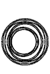
Figure 1. The Julia set of the $2$-generator polynomial semigroup $G_{\lambda_{0}}$ with $(d_{1},d_{2})=(3,2),b=0.1$, in Theorem 1.4. $G_{\lambda_{0}}$ satisfies the open set condition, $J(G_{\lambda_{0}})$ is connected and $\text{{\rm HD}}(J(G_{\lambda_{0}}))=s(\lambda_{0})<2.$

In Theorem 1.4 we deal with $2$-generator polynomial semigroups $\langle\gamma_{1},\gamma_{2}\rangle$ with $\deg(\gamma_{1}),$ $\deg(\gamma_{2})$ $\geq 2$, $(\deg(\gamma_{1}),\deg(\gamma_{2}))\neq(2,2)$ for which the planar postcritical set is bounded. In fact, it is very important to investigate the dynamics of polynomial semigroups with bounded planar postcritical set (see [31, 38, 32, 23]). There appear many new phenomena (for example, the Julia sets of such semigroups can be disconnected) in the dynamics of such semigroups which cannot hold in the usual iteration dynamics of a single polynomial. In the proof of Theorem 1.4, we use some idea from the study of dynamics of such semigroups. In the family of Theorem 1.4, for a typical parameter value the Hausdorff dimension of the Julia set is strictly less than $2$ and is equal to the Bowen parameter. Thus it is very natural to ask what happens for polynomial semigroups $\langle\gamma_{1},\gamma_{2}\rangle$ with $\deg(\gamma_{1})=\deg(\gamma_{2})=2$ for which the planar postcritical set is bounded. In this case, by [31, Theorem 2.15], $J(\langle\gamma_{1},\gamma_{2}\rangle)$ is connected and $\gamma_{1}^{-1}(J(\langle\gamma_{1},\gamma_{2}\rangle))\cap\gamma_{2}^{-1}(J(\langle\gamma_{1},\gamma_{2}\rangle))\neq\emptyset.$ Combining Proposition 1.3 and the lower estimate of the Bowen parameter from [41], which was obtained by using thermodynamic formalisms, potential theory, and some results from [43], we prove the following.

Theorem 1.6 (Corollary 4.5).

For each $a\in{\mathbb{C}}$ with $|a|\neq 0,1$, there exists an open neighborhood $Y_{a}$ of $(az^{2},z^{2})$ in ${\mathcal{P}}^{2}$ such that $\{g=(g_{1},g_{2})\}_{g\in Y_{a}}$ is a holomorphic family in $\text{{\rm Exp}}(2)$ satisfying the analytic transversality condition, the strong transversality condition and the transversality condition, and for a.e. $g=(g_{1},g_{2})\in Y_{a}$ with respect to the Lebesgue measure on ${\mathcal{P}}^{2}$, we have that $\mbox{{\em Leb}}_{2}(J(\langle g_{1},g_{2}\rangle))>0.$

Note that in the usual iteration dynamics of a single expanding rational map $g$, the Hausdorff dimension of the Julia set is strictly less than two. In particular, Leb${}_{2}(J(g))=0.$

For any $a\in{\mathbb{C}}$ with $|a|\neq 0,1$, $J(\langle az^{2},z^{2}\rangle)$ is equal to the closed annulus between $\{w\in{\mathbb{C}}:|w|=1\}$ and $\{w\in{\mathbb{C}}:|w|=|a|^{-1}\}$, thus $\mbox{int}(J(\langle az^{2},z^{2}\rangle))\neq\emptyset.$ However, regarding Theorem 1.6, it is an open problem to determine, for any other parameter value $(g_{1},g_{2})\in Y_{a}$ with $\mbox{Leb}_{2}(J(\langle g_{1},g_{2}\rangle))>0$, whether $\mbox{int}(J(\langle g_{1},g_{2}\rangle))=\emptyset$ or not. We have some partial answers though. At least we can show that for each $a\in{\mathbb{C}}$ with $|a|\neq 0,1$ and for each neighborhood $W$ of $(az^{2},z^{2})$ in $Y_{a}$ there exists a non-empty open subset $\tilde{W}$ of $W$ such that for each $(\gamma_{1},\gamma_{2})\in\tilde{W}$, the Fatou set $F(\langle\gamma_{1},\gamma_{2}\rangle)$ has at least three connected components, and thus the Julia set $J(\langle\gamma_{1},\gamma_{2}\rangle)$ is not a closed annulus. If $a\in{\mathbb{R}}$ with $a>0,a\neq 1$, then we can show that for each neighborhood $W$ of $(az^{2},z^{2})$ in $Y_{a}$ and for each $n\in{\mathbb{N}}$ with $n\geq 3$, there exists a non-empty open subset $W_{n}$ of $W$ such that for each $(\gamma_{1},\gamma_{2})\in W_{n}$, $F(\langle\gamma_{1},\gamma_{2}\rangle)$ has at least $n$ connected components and $J(\langle\gamma_{1},\gamma_{2}\rangle)$ is not a closed annulus (see Remark 4.6).

We now consider the expanding semigroups generated by affine maps. Let $m\geq 2.$ For each $j=1,\ldots,m$, let $g_{j}(z)=a_{j}z+b_{j}$, where $a_{j},b_{j}\in{\mathbb{C}},|a_{j}|>1.$ Let $G=\langle g_{1},\ldots,g_{m}\rangle.$ Since $|a_{j}|>1$, $\infty\in F(G).$ Hence, by (1.1), $J(G)$ is a compact subset of ${\mathbb{C}}$ which satisfies $J(G)=\bigcup_{j=1}^{m}g_{j}^{-1}(J(G)).$ Since $g_{j}^{-1}$ is a contracting similitude on ${\mathbb{C}}$, it follows that $J(G)$ is equal to the self-similar set constructed by the family $\{g_{1}^{-1},\ldots,g_{m}^{-1}\}$ of contracting similitudes. For the definition of self-similar sets, see [4, 5, 9]. Note that the Bowen parameter $\delta(g_{1},\ldots,g_{m})$ of $(g_{1},\ldots,g_{m})$ is equal to the unique solution of the equation $\sum_{i=1}^{m}|a_{i}|^{-t}=1,\,t\geq 0$. Thus $\delta(g_{1},\ldots,g_{m})$ is the similarity dimension of $\{g_{1}^{-1},\ldots,g_{m}^{-1}\}.$ Conversely, any self-similar set constructed by a finite family $\{h_{1},\ldots,h_{m}\}$ of contracting similitudes on ${\mathbb{C}}$ is equal to the Julia set of the rational semigroup $\langle h_{1}^{-1},\ldots,h_{m}^{-1}\rangle.$ By using Proposition 1.3 and some calculations of the partial derivatives of the conjugacy maps with respect to the parameters, we prove the following.

Theorem 1.7 (Theorem 4.8).

Let $m\in{\mathbb{N}}$ with $m\geq 2.$ For each $i=1,\ldots,m,$, let $g_{i}(z)=a_{i}z+b_{i},$ where $a_{i}\in{\mathbb{C}},\,|a_{i}|>1$, $b_{i}\in{\mathbb{C}}$. Let $G:=\langle g_{1},\ldots,g_{m}\rangle.$ We suppose all of the following conditions hold.

• For each $(i,j)$ with $i\neq j$ and $g_{i}^{-1}(J(G))\cap g_{j}^{-1}(J(G))\neq\emptyset$, there exists a number $\alpha_{ij}\in\{1,\ldots,m\}$ such that $g_{i}(g_{i}^{-1}(J(G))\cap g_{j}^{-1}(J(G)))\subset\{\frac{-b_{\alpha_{ij}}}{a_{\alpha_{ij}}-1}\}.$

• If $i,j,k$ are mutually distinct elements in $\{1,\ldots,m\}$, then

  $$g_{k}(g_{i}^{-1}(J(G))\cap g_{j}^{-1}(J(G)))\subset F(G).$$

• For each $(j,k)$ with $j\neq k$, we have $g_{k}(\frac{-b_{j}}{a_{j}-1})\in F(G).$

Then, there exists an open neighborhood $U$ of $(g_{1},\ldots,g_{m})\in(\mbox{{\em Aut}}({\mathbb{C}}))^{m}$, where Aut$({\mathbb{C}}):=\{az+b:a\in{\mathbb{C}}\setminus\{0\},b\in{\mathbb{C}}\}$, such that $\{\gamma=(\gamma_{1},\ldots,\gamma_{m})\}_{\gamma\in U}$ is a holomorphic family in $\text{{\rm Exp}}(m)$ satisfying the analytic transversality condition, the strong transversality condition and the transversality condition.

Note that in the above theorem, for each $j=1,\ldots,m$, $J(g_{j})=\{\frac{-b_{j}}{a_{j}-1}\}.$

Note also that even if we replace “$\mbox{Aut}({\mathbb{C}})$” by $\mbox{Aut}({\hat{\mathbb{C}}}):=\{\frac{az+b}{cz+d}:a,b,c,d,\in{\mathbb{C}},ad-bc\neq 0\}$, similar results hold (see Remark 4.9).

By using Theorem 1.7, we can obtain many examples of families of systems of affine maps satisfying the analytic transversality condition. In fact, we have the following.

Example 1.8 (Example 4.11).

Let $p_{1},p_{2},p_{3}\in{\mathbb{C}}$ be such that $p_{1}p_{2}p_{3}$ makes an equilateral triangle. For each $i=1,2,3$, let $g_{i}(z)=2(z-p_{i})+p_{i}.$ Let $G=\langle g_{1},g_{2},g_{3}\rangle.$ Then $J(G)$ is equal to the Sierpinski gasket. It is easy to see that $(g_{1},g_{2},g_{3})$ satisfies the assumptions of Theorem 1.7. Moreover, $\delta(g_{1},g_{2},g_{3})=\text{{\rm HD}}(J(G))=\frac{\log 3}{\log 2}<2.$ By Theorems 1.7, 1.2 and 2.15, there exists an open neighborhood $U$ of $(g_{1},g_{2},g_{3})$ in $(\mbox{{\em Aut}}({\mathbb{C}}))^{3}$ and a Borel subset $A$ of $U$ with $\text{{\rm HD}}(U\setminus A)<\text{{\rm HD}}(U)=12$ such that (1) $\{\gamma=(\gamma_{1},\gamma_{2},\gamma_{3})\}_{\gamma\in U}$ is a holomorphic family in $\text{{\rm Exp}}(3)$ satisfying the analytic transversality condition, the strong transversality condition and the transversality condition, and (2) for each $\gamma=(\gamma_{1},\gamma_{2},\gamma_{3})\in A$, $\text{{\rm HD}}(J(\langle\gamma_{1},\gamma_{2},\gamma_{3}\rangle))=\delta(\gamma_{1},\gamma_{2},\gamma_{3})<2.$

For some other examples including the families related to the Snowflake, Pentakun, Hexakun, Heptakun, Octakun and so on, see Examples 4.10, 4.13, 4.14, 4.15 and Remark 4.16. (For the definition of Snowflake, Pentakun, etc., see [9].) We remark that, up to our best knowledge, these examples (Examples 1.8, etc.) have not been explicitly dealt with in any literature of contracting IFSs with overlaps.

In section 2, we introduce and collect some fundamental concepts, notation, and definitions. In section 3, we prove the main results of this paper. In section 4, we describe some applications and examples. In section 5, we make a remark on similar results for families of conformal contracting iterated function systems in arbitrary dimensions.

2. Preliminaries

In this section we introduce notation and basic definitions. Throughout the paper, we frequently follow the notation from [26] and [28].

Definition 2.1 ([8, 44]).

A “rational semigroup” $G$ is a semigroup generated by a family of non-constant rational maps $g:{\hat{\mathbb{C}}}\rightarrow{\hat{\mathbb{C}}}$, where ${\hat{\mathbb{C}}}$ denotes the Riemann sphere, with the semigroup operation being functional composition. A “polynomial semigroup” is a semigroup generated by a family of non-constant polynomial maps of ${\hat{\mathbb{C}}}.$ For a rational semigroup $G$, we set

$$F(G):=\{z\in{\hat{\mathbb{C}}}:G\mbox{ is normal in some neighborhood of }z\}$$

and we call $F(G)$ the Fatou set of $G$. Its complement,

$$J(G):={\hat{\mathbb{C}}}\setminus F(G)$$

is called the Julia set of $G.$ If $G$ is generated by a family $\{f_{i}\}_{i}$ (i.e., $G=\{f_{i_{1}}\circ\cdots\circ f_{i_{n}}:n\in{\mathbb{N}},\forall f_{i_{j}}\in\{f_{i}\}\}$), then we write $G=\langle f_{1},f_{2},\ldots\rangle.$ For each $g\in\mbox{{\em Rat}}$, we set $F(g):=F(\langle g\rangle)$ and $J(g):=J(\langle g\rangle).$

Note that for each $h\in G$, $h(F(G))\subset F(G),h^{-1}(J(G))\subset J(G).$ For the fundamental properties of $F(G)$ and $J(G)$, see [8, 22, 26]. For the papers dealing with dynamics of rational semigroups, see for example [8, 44, 22, 24, 25, 26, 27, 28, 29, 30, 40, 39, 41, 31, 38, 32, 23, 33, 34, 35, 36, 37], etc.

We denote by Rat the set of all non-constant rational maps on ${\hat{\mathbb{C}}}$ endowed with distance $\overline{d}$ defined by $\overline{d}(h_{1},h_{2}):=\sup_{z\in{\hat{\mathbb{C}}}}\hat{\rho}(h_{1}(z),h_{2}(z))$, where $\hat{\rho}$ denotes the spherical distance on ${\hat{\mathbb{C}}}.$ For each $d\in{\mathbb{N}}$, we set Rat${}_{d}:=\{g\in\mbox{Rat}:\deg(g)=d\}.$ Note that each $\mbox{Rat}_{d}$ is a connected component of Rat. Hence Rat has countably many connected components. In addition, each connected component $\mbox{Rat}_{d}$ of Rat is an open subset of Rat and $\mbox{Rat}_{d}$ has a structure of a finite dimensional complex manifold. Similarly, we denote by ${\mathcal{P}}$ the set of all polynomial maps $g:{\hat{\mathbb{C}}}\rightarrow{\hat{\mathbb{C}}}$ with $\deg(g)\geq 2$ endowed with the relative topology inherited from Rat. We set $\mbox{Aut}({\mathbb{C}}):=\{az+b:a,b\in{\mathbb{C}},a\neq 0\}$ endowed with the relative topology inherited from Rat. For each $d\in{\mathbb{N}}$ with $d\geq 2$, we set ${\mathcal{P}}_{d}:=\{g\in{\mathcal{P}}:\deg(g)=d\}.$ Note that each ${\mathcal{P}}_{d}$ is a connected component of ${\mathcal{P}}.$ Hence ${\mathcal{P}}$ has countably many connected components. In addition, each connected component ${\mathcal{P}}_{d}$ of ${\mathcal{P}}$ is an open subset of ${\mathcal{P}}$ and ${\mathcal{P}}_{d}$ has a structure of a finite dimensional complex manifold. Moreover, Aut$({\mathbb{C}})$ is a connected, complex-two-dimensional complex manifold. We remark that $g_{n}\rightarrow g$ as $n\rightarrow\infty$ in ${\mathcal{P}}\cup\mbox{Aut}({\mathbb{C}})$ if and only if there exists a number $N\in{\mathbb{N}}$ such that

• $\deg(g_{n})=\deg(g)$ for each $n\geq N$, and

• the coefficients of $g_{n}(n\geq N)$ converge to the coefficients of $g$ appropriately as $n\rightarrow\infty.$

Thus

$${\mathcal{P}}_{d}\cong({\mathbb{C}}\setminus\{0\})\times{\mathbb{C}}^{d}\ \text{ and }\ \mbox{Aut}({\mathbb{C}})\cong({\mathbb{C}}\setminus\{0\})\times{\mathbb{C}}.$$

For more information on the topology and complex structure of Rat and ${\mathcal{P}}\cup\mbox{Aut}({\mathbb{C}})$, the reader may consult [2].

For each $z\in{\hat{\mathbb{C}}}$, we denote by $T{\hat{\mathbb{C}}}_{z}$ the complex tangent space of ${\hat{\mathbb{C}}}$ at $z.$ Let $\varphi:V\rightarrow{\hat{\mathbb{C}}}$ be a holomorphic map defined on an open set $V$ of ${\hat{\mathbb{C}}}$ and let $z\in V.$ We denote by $D\varphi_{z}:T{\hat{\mathbb{C}}}_{z}\rightarrow T{\hat{\mathbb{C}}}_{\varphi(z)}$ the derivative of $\varphi$ at $z.$ Moreover, we denote by $\|\varphi^{\prime}(z)\|$ the norm of the derivative $D\varphi_{z}$ at $z$ with respect to the spherical metric on ${\hat{\mathbb{C}}}.$

Definition 2.2.

For each $m\in\mathbb{N}$, let $\Sigma_{m}:=\{1,\ldots,m\}^{\mathbb{N}}$ be the space of one-sided sequences of $m$-symbols endowed with the product topology. This is a compact metrizable space. For each $f=(f_{1},\ldots,f_{m})\in(\mbox{{\em Rat}})^{m}$, we define a map

$$\tilde{f}:\Sigma_{m}\times{\hat{\mathbb{C}}}\rightarrow\Sigma_{m}\times{\hat{\mathbb{C}}}$$

by the formula

$$\tilde{f}(\omega,z)=(\sigma(\omega),\ f_{\omega_{1}}(z)),$$

where $(\omega,z)\in\Sigma_{m}\times{\hat{\mathbb{C}}},\ \omega=(\omega_{1},\omega_{2},\ldots),$ and $\sigma:\Sigma_{m}\rightarrow\Sigma_{m}$ denotes the shift map. The transformation $\tilde{f}:\Sigma_{m}\times{\hat{\mathbb{C}}}\rightarrow\Sigma_{m}\times{\hat{\mathbb{C}}}$ is called the skew product map associated with the multimap $f=(f_{1},\ldots,f_{m})\in(\mbox{{\em Rat}})^{m}.$ We denote by $\pi_{1}:\Sigma_{m}\times{\hat{\mathbb{C}}}\rightarrow\Sigma_{m}$ the projection onto $\Sigma_{m}$ and by $\pi_{2}:\Sigma_{m}\times{\hat{\mathbb{C}}}\rightarrow{\hat{\mathbb{C}}}$ the projection onto ${\hat{\mathbb{C}}}$. That is, $\pi_{1}(\omega,z)=\omega$ and $\pi_{2}(\omega,z)=z.$ For each $n\in\mathbb{N}$ and $(\omega,z)\in\Sigma_{m}\times{\hat{\mathbb{C}}}$, we put

$$\|(\tilde{f}^{n})^{\prime}(\omega,z)\|:=\|(f_{\omega_{n}}\circ\cdots\circ f_{\omega_{1}})^{\prime}(z)\|.$$

We define

$$J_{\omega}(\tilde{f}):=\{z\in{\hat{\mathbb{C}}}:\{f_{\omega_{n}}\circ\cdots\circ f_{\omega_{1}}\}_{n\in\mathbb{N}}\mbox{ is not normal in any neighborhood of }z\}$$

for each $\omega\in\Sigma_{m}$ and we set

$$J(\tilde{f}):=\overline{\cup_{w\in\Sigma_{m}}\{\omega\}\times J_{\omega}(\tilde{f})},$$

where the closure is taken with respect to the product topology on the space $\Sigma_{m}\times{\hat{\mathbb{C}}}.$ $J(\tilde{f})$ is called the Julia set of the skew product map $\tilde{f}.$ In addition, we set $F(\tilde{f}):=(\Sigma_{m}\times{\hat{\mathbb{C}}})\setminus J(\tilde{f})$ and $\deg(\tilde{f}):=\sum_{j=1}^{m}\deg(f_{j}).$ We also set $\Sigma_{m}^{\ast}:=\cup_{j=1}^{\infty}\{1,\ldots,m\}^{j}$ (disjoint union). For each $\omega\in\Sigma_{m}\cup\Sigma_{m}^{*}$ let $|\omega|$ be the length of $\omega.$ For each $\omega\in\Sigma_{m}\cup\Sigma_{m}^{*}$ we write $\omega=(\omega_{1},\omega_{2},\ldots).$ For each $f=(f_{1},\ldots,f_{m})\in(\mbox{{\em Rat}})^{m}$ and each $\omega=(\omega_{1},\ldots,\omega_{n})\in\Sigma_{m}^{\ast}$, we put

$$f_{\omega}:=f_{\omega_{n}}\circ\cdots\circ f_{\omega_{1}}.$$

For every $n\leq|\omega|$ let $\omega|_{n}=(\omega_{1},\omega_{2},\ldots,\omega_{n})$. If $\omega\in\Sigma_{m}^{*}$, we put

$$[\omega]=\{\tau\in\Sigma_{m}:\tau|_{|\omega|}=\omega\}.$$

If $\omega,\tau\in\Sigma_{m}\cup\Sigma_{m}^{*}$, $\omega\wedge\tau$ is the longest initial subword common for both $\omega$ and $\tau$. Let $\alpha$ be a fixed number with $0<\alpha<1/2.$ We endow the shift space $\Sigma_{m}$ with the distance $\rho_{\alpha}$ defined as $\rho_{\alpha}(\omega,\tau)=\alpha^{|\omega\wedge\tau|}$ with the standard convention that $\alpha^{\infty}=0$. The distance $\rho_{\alpha}$ induces the product topology on $\Sigma_{m}$. Denote the spherical distance on ${\hat{\mathbb{C}}}$ by $\hat{\rho}$ and equip the product space $\Sigma_{m}\times{\hat{\mathbb{C}}}$ with the distance $\rho$ defined as follows.

$$\rho((\omega,x),(\tau,y))=\max\{\rho_{\alpha}(\omega,\tau),\hat{\rho}(x,y)\}.$$

Of course $\rho$ induces the product topology on $\Sigma_{m}\times{\hat{\mathbb{C}}}$. If $\omega=(\omega_{1},\omega_{2},\ldots,\omega_{n})\in\Sigma_{m}^{\ast}$ and $\tau=(\tau_{1},\tau_{2},\ldots)\in\Sigma_{m}^{\ast}\cup\Sigma_{m}$, we set $\omega\tau:=(\omega_{1},\omega_{2},\ldots,\omega_{n},\tau_{1},\tau_{2},\ldots)\in\Sigma_{m}^{\ast}\cup\Sigma_{m}.$ For a $j\in\{1,\ldots,m\}$, we set $j^{\infty}:=(j,j,j,\ldots)\in\Sigma_{m}.$

Remark 2.3.

By definition, the set $J(\tilde{f})$ is compact. Furthermore, if we set $G=\langle f_{1},\ldots,f_{m}\rangle$, then, by [26, Proposition 3.2], the following hold:

1. $J(\tilde{f})$ is completely invariant under $\tilde{f}$;

2. $\tilde{f}$ is an open map on $J(\tilde{f})$;

3. if $\sharp J(G)\geq 3$ and $E(G):=\{z\in{\hat{\mathbb{C}}}:\sharp\cup_{g\in G}g^{-1}(\{z\})<\infty\}$ is contained in $F(G)$, then the dynamical system $(\tilde{f},J(\tilde{f}))$ is topologically exact;

4. $J(\tilde{f})$ is equal to the closure of the set of repelling periodic points of $\tilde{f}$ if $\sharp J(G)\geq 3$, where we say that a periodic point $(\omega,z)$ of $\tilde{f}$ with period $n$ is repelling if $\|(\tilde{f}^{n})^{\prime}(\omega,z)\|>1$.

5. $\pi_{2}(J(\tilde{f}))=J(G).$

Definition 2.4 ([28]).

A finitely generated rational semigroup $G=\langle f_{1},\ldots,f_{m}\rangle$ is said to be expanding provided that $J(G)\neq\emptyset$ and the skew product map $\tilde{f}:\Sigma_{m}\times{\hat{\mathbb{C}}}\rightarrow\Sigma_{m}\times{\hat{\mathbb{C}}}$ associated with $f=(f_{1},\ldots,f_{m})$ is expanding along fibers of the Julia set $J(\tilde{f})$, meaning that there exist $\eta>1$ and $C\in(0,1]$ such that for all $n\geq 1$,

(2.1) $$\inf\{\|(\tilde{f}^{n})^{\prime}(z)\|:z\in J(\tilde{f})\}\geq C\eta^{n}.$$

Definition 2.5.

Let $G$ be a rational semigroup. We put

$$P(G):=\overline{\cup_{g\in G}\{\mbox{all critical values of }g:{\hat{\mathbb{C}}}\rightarrow{\hat{\mathbb{C}}}\}}\ (\subset{\hat{\mathbb{C}}})$$

and we call $P(G)$ the postcritical set of $G$. A rational semigroup $G$ is said to be hyperbolic if $P(G)\subset F(G).$

We remark that if $\Gamma\subset\mbox{Rat}$ and $G$ is generated by $\Gamma$, then

(2.2) $$P(G)=\overline{\bigcup_{g\in G\cup\{Id\}}g(\bigcup_{h\in\Gamma}\{\mbox{all critical values of }h:{\hat{\mathbb{C}}}\rightarrow{\hat{\mathbb{C}}}\})}.$$

Therefore for each $g\in G$, $g(P(G))\subset P(G).$

Definition 2.6.

Let $G$ be a polynomial semigroup. We set $P^{\ast}(G):=P(G)\setminus\{\infty\}.$ This set is called the planar postcritical set of $G.$ We say that $G$ is postcritically bounded if $P^{\ast}(G)$ is bounded in ${\mathbb{C}}.$

Remark 2.7.

Let $G=\langle f_{1},\ldots,f_{m}\rangle$ be a rational semigroup such that there exists an element $g\in G$ with $\deg(g)\geq 2$ and such that each Möbius transformation in $G$ is loxodromic. Then, it was proved in [25] that $G$ is expanding if and only if $G$ is hyperbolic.

Definition 2.8.

For each $m\in{\mathbb{N}}$, we define

$$\text{{\rm Exp}}(m):=\{(f_{1},\ldots,f_{m})\in(\mbox{{\em Rat}})^{m}:\langle f_{1},\ldots,f_{m}\rangle\mbox{ is expanding}\}.$$

Then we have the following.

Lemma 2.9 ([24, 40]).

$\text{{\rm Exp}}(m)$ is an open subset of (Rat$)^{m}.$

Lemma 2.10 (Theorem 2.14 in [27]).

For each $f=(f_{1},\ldots,f_{m})\in\text{{\rm Exp}}(m)$, $J(\tilde{f})=\bigcup_{\omega\in\Sigma_{m}}(\{\omega\}\times J_{\omega}(\tilde{f}))$ and $J(\langle f_{1},\ldots,f_{m}\rangle)=\bigcup_{\omega\in\Sigma_{m}}J_{\omega}(\tilde{f}).$

Definition 2.11.

We set

$$\text{{\rm Epb}}(m):=\{f=(f_{1},\ldots,f_{m})\in\text{{\rm Exp}}(m)\cap{\mathcal{P}}^{m}:\langle f_{1},\ldots,f_{m}\rangle\mbox{ is postcritically bounded}\}.$$

Lemma 2.12 ([32, 34]).

$\text{{\rm Epb}}(m)$ is open in ${\mathcal{P}}^{m}.$

Definition 2.13.

Let $f=(f_{1},\ldots,f_{m})\in\text{{\rm Exp}}(m)$ and let $\tilde{f}:\Sigma_{m}\times{\hat{\mathbb{C}}}\rightarrow\Sigma_{m}\times{\hat{\mathbb{C}}}$ be the skew product map associated with $f=(f_{1},\ldots,f_{m}).$ For each $t\in{\mathbb{R}}$, let $P(t,f)$ be the topological pressure of the potential $\varphi(z):=-t\log\|\tilde{f}^{\prime}(z)\|$ with respect to the map $\tilde{f}:J(\tilde{f})\rightarrow J(\tilde{f}).$ (For the definition of the topological pressure, see [18].) We denote by $\delta(f)$ the unique zero of the function ${\mathbb{R}}\ni t\mapsto P(t,f)\in{\mathbb{R}}.$ Note that the existence and uniqueness of the zero of the function $P(t,f)$ was shown in [28]. The number $\delta(f)$ is called the Bowen parameter of the multimap $f=(f_{1},\ldots,f_{m})\in\text{{\rm Exp}}(m).$

Let $u\geq 0$. A Borel probability measure $\mu$ on $J(\tilde{f})$ is said to be $u$-conformal for $\tilde{f}$ if the following holds. For any Borel subset $A$ of $J(\tilde{f})$ such that $\tilde{f}|_{A}:A\rightarrow J(\tilde{f})$ is injective, we have that

$$\mu(\tilde{f}(A))=\int_{A}\|\tilde{f}^{\prime}(z)\|^{u}d\mu(z).$$

We remark that with the notation of Definition 2.13, there exists a unique $\delta(f)$-conformal measure for $\tilde{f}$ (see [28]).

Definition 2.14.

For a subset $A$ of ${\hat{\mathbb{C}}}$, we denote by $\text{{\rm HD}}(A)$ the Hausdorff dimension of $A$ with respect to the spherical distance. For each $d\in{\mathbb{N}}$, if $B$ is a subset of ${\mathbb{R}}^{d}$, we denote by $\text{{\rm HD}}(B)$ the Hausdorff dimension of $B$ with respect to the Euclidean distance on ${\mathbb{R}}^{d}.$ For a Riemann surface $S$, we denote by $\mbox{{\em Aut}}(S)$ the set of all holomorphic isomorphisms of $S.$ For a compact metric space $X$, we denote by $C(X)$ the Banach space of all continuous complex-valued functions on $X$, endowed with the supremum norm.

A fundamental fact about the Bowen parameter is the following.

Theorem 2.15 ([28, 25]).

For each $f=(f_{1},\ldots,f_{m})\in\text{{\rm Exp}}(m)$, $\text{{\rm HD}}(J(\langle f_{1},\ldots,f_{m}\rangle))\leq\delta(f).$

Another crucial property of the Bowen parameter is the following fact proved as one of the main results of [40].

Theorem 2.16 ([40]).

The function $\text{{\rm Exp}}(m)\ni f\mapsto\delta(f)\in{\mathbb{R}}$ is real-analytic and plurisubharmonic.

Remark 2.17 ([28, 41]).

Let $f=(f_{1},\ldots,f_{m})\in\text{{\rm Exp}}(m).$ Then there exists a unique equilibrium state $\nu_{f}$ with respect to $\tilde{f}:J(\tilde{f})\rightarrow J(\tilde{f})$ for the potential function $-\delta(f)\log\|\tilde{f}^{\prime}(z)\|.$ The $\tilde{f}$-invariant probability measure $\nu_{f}$ is equivalent to the $\delta(f)$-conformal measure for $\tilde{f}.$ We have that $\delta(f)=\frac{h_{\nu_{f}}(\tilde{f})}{\int\log\|\tilde{f}^{\prime}\|d\nu_{f}}$, where $h_{\nu_{f}}(\tilde{f})$ denotes the metric entropy of $(\tilde{f},\nu_{f}).$ Moreover, $\delta(f)$ is equal to the “critical exponent of the Poincaré series” of the multimap $f$. For the details, see [28, 41].

3. Proofs and Results

In this section we state and prove the main results of our paper.

Definition 3.1.

Let $f=(f_{1},\ldots,f_{m})\in(\mbox{{\em Rat}})^{m}$ and let $G=\langle f_{1},\ldots,f_{m}\rangle$. Let also $U$ be a non-empty open set in ${\hat{\mathbb{C}}}.$ We say that $f$ (or $G$) satisfies the open set condition (with $U$) if

$$\cup_{j=1}^{m}f_{j}^{-1}(U)\subset U\ \text{ and }\ f_{i}^{-1}(U)\cap f_{j}^{-1}(U)=\emptyset$$

for each $(i,j)$ with $i\neq j.$ There is also a stronger condition. Namely, we say that $f$ (or $G$) satisfies the separating open set condition (with $U$) if

$$\cup_{j=1}^{m}f_{j}^{-1}(U)\subset U\ \text{ and }\ f_{i}^{-1}(\overline{U})\cap f_{j}^{-1}(\overline{U})=\emptyset$$

for each $(i,j)$ with $i\neq j.$

We remark that the above concept of “open set condition” (for “backward IFSs”) is an analogue of the usual open set condition in the theory of IFSs.

The following theorem is important for our investigations.

Theorem 3.2 ([28]).

Let $f=(f_{1},\ldots,f_{m})\in\text{{\rm Exp}}(m)$. If $f$ satisfies the open set condition, then $\text{{\rm HD}}(J(\langle f_{1},\ldots,f_{m}\rangle))=\delta(f).$

It is interesting to ask for an estimate of the Hausdorff dimension of the Julia set of $G$ in the case when it is not known whether $G$ satisfies the open set condition or not. The goal of our paper is to provide answers to this question. We start with introducing the following setting.

Setting $(\ast)$: Let $d,m\in{\mathbb{N}}$. Let $U$ be a non-empty bounded open subset of ${\mathbb{R}}^{d}.$ For each $\lambda\in U$, let $f_{\lambda}=(f_{\lambda,1},\ldots,f_{\lambda,m})\in\text{{\rm Exp}}(m)$ and let $G_{\lambda}:=\langle f_{\lambda,1},\ldots,f_{\lambda,m}\rangle.$ We suppose that $\{f_{\lambda}\}_{\lambda\in U}$ is a continuous family of $\text{{\rm Exp}}(m)$, i.e., the map $U\ni\lambda\mapsto f_{\lambda}\in\text{{\rm Exp}}(m)$ is continuous. Fix a parameter $\lambda_{0}\in U$. Suppose that for each $\lambda\in U$, there exists a homeomorphism $h_{\lambda}:J(\tilde{f}_{\lambda_{0}})\rightarrow J(\tilde{f}_{\lambda})$ of the form $h_{\lambda}(\omega,z)=(\omega,\overline{h}_{\lambda}(\omega,z))$ such that $h_{\lambda_{0}}=Id|_{J(\tilde{f}_{\lambda_{0}})}$, $h_{\lambda}\circ\tilde{f}_{\lambda_{0}}=\tilde{f}_{\lambda}\circ h_{\lambda}$ on $J(\tilde{f}_{\lambda_{0}})$, and such that the map $(\omega,z,\lambda)\mapsto\overline{h}_{\lambda}(\omega,z)\in{\hat{\mathbb{C}}},(\omega,z,\lambda)\in J(\tilde{f}_{\lambda_{0}})\times U$, is continuous. The point $\lambda_{0}$ is called the base point of $\{f_{\lambda}\}_{\lambda\in U}.$ Let $C>0,\eta>1$ be such that for each $n\in{\mathbb{N}}$, $\inf_{(\omega,z)\in J(\tilde{f}_{\lambda_{0}})}\|(\tilde{f}^{n}_{\lambda_{0}})^{\prime}(\omega,z)\|\geq C\eta^{n}.$ For each $\lambda\in U$, we set $s(\lambda):=\delta(f_{\lambda})$, where $\delta(f_{\lambda})$ is the Bowen parameter of the multimap $f_{\lambda}.$

We now will explain (in Definition 3.3 and Remark 3.4) that Setting $(\ast)$ is natural.

Definition 3.3.

Let $M$ be a finite dimensional complex manifold. Let $m\in{\mathbb{N}}.$ For each $\lambda\in M$, let $f_{\lambda}=(f_{\lambda,1},\ldots,f_{\lambda,m})$ be an element of $\text{{\rm Exp}}(m).$ We say that $\{f_{\lambda}\}_{\lambda\in M}$ is a holomorphic family in $\text{{\rm Exp}}(m)$ over $M$ if the map $\lambda\mapsto f_{\lambda}\in\text{{\rm Exp}}(m),\lambda\in M$, is holomorphic. If a holomorphic family $\{f_{\lambda}\}_{\lambda\in M}$ in $\text{{\rm Exp}}(m)$ satisfies that $f_{\lambda}\in\text{{\rm Epb}}(m)$ for each $\lambda\in M$, then we say that $\{f_{\lambda}\}_{\lambda\in M}$ is a holomorphic family in $\text{{\rm Epb}}(m).$

Remark 3.4.

Let $\{f_{\lambda}\}_{\lambda\in M}$ be a holomorphic family in $\text{{\rm Exp}}(m)$ over a complex manifold $M$ and let $\lambda_{0}\in M.$ Then there exists a neighborhood $U$ of $\lambda_{0}$ such that for the holomorphic family $\{f_{\lambda}\}_{\lambda\in U}$ over $U$, there exists a unique family $\{h_{\lambda}\}_{\lambda\in U}$ of conjugacy maps as in Setting $(\ast).$ Moreover, $\lambda\mapsto\overline{h}_{\lambda}(\omega,z)$ is holomorphic. For the proof of this result, see [40, Theorem 4.9, Lemma 6.2] and its proof (in fact, the assumption “ $f$ is simple” in [40, Theorem 4.9] is not needed).

Remark 3.5.

Let $\{f_{\lambda}\}_{\lambda\in M}$ be a holomorphic family in $\text{{\rm Exp}}(m)$ over $M$ and let $\lambda_{0}\in M$. Since the map $\lambda\mapsto J(G_{\lambda})$ is continuous with respect to the Hausdorff metric ([24, Theorem 2.3.4], [40, Lemma 4.1]), there exist a Möbius transformation $\alpha$, an open neighborhood $U$ of $\lambda_{0}$, and a compact subset $K$ of ${\mathbb{C}}$ such that setting $\tilde{G}_{\lambda}:=\{\alpha\circ g\circ\alpha^{-1}:g\in G_{\lambda}\}$ for each $\lambda\in U$, we have $J(\tilde{G}_{\lambda})\subset K$ for each $\lambda\in U.$

From Lemma 3.6 through Theorem 3.12, we assume Setting $(\ast)$.

Notation: For a $x\in{\mathbb{R}}^{d}$ and $r>0$, we denote by $B_{r}(x)$ the open $r$-ball with center $x$ with respect to the Euclidean distance. For a $y\in{\mathbb{C}}$ and $r>0$ we set $D_{r}(y):=\{z\in{\mathbb{C}}:|z-y|<r\}.$ We denote by Leb_d the $d$-dimensional Lebesgue measure on a $d$-dimensional manifold.

Under Setting $(\ast)$, the following lemma is immediate.

Lemma 3.6.

Let $s,\epsilon>0$ be given with $s>\epsilon.$ Then there exist constants $v>0$ and $\delta>0$ such that for any $(\omega,z,\omega^{\prime},z^{\prime},\lambda)\in J(\tilde{f}_{\lambda_{0}})^{2}\times U$, if $\rho((\omega,z),(\omega^{\prime},z^{\prime}))<v$ and $\lambda\in B_{\delta}(\lambda_{0})$, then

• $(\eta^{\frac{3\epsilon}{4(s-\epsilon)}})^{-1}\leq\frac{\|\tilde{f}_{\lambda}^{\prime}(\omega^{\prime},z^{\prime})\|}{\|\tilde{f}_{\lambda_{0}}^{\prime}(\omega,z)\|}\leq\min\{\eta^{\frac{3\epsilon}{4(s-\epsilon)}},\eta^{\frac{\epsilon}{4}}\}$ and

• $\hat{\rho}(z,\overline{h}_{\lambda}(\omega,z))<\frac{1}{2}v.$

We now give the definition of the transversality condition, the concept of our primary interests in this paper.

Definition 3.7.

Let $\{f_{\lambda}\}_{\lambda\in U}$ be as in Setting $(\ast).$ We say that $\{f_{\lambda}\}_{\lambda\in U}$ satisfies the transversality condition (TC) if there exists a constant $C_{1}>0$ such that for each $r\in(0,\mbox{{\em diam}}({\hat{\mathbb{C}}}))$ and for each $(\omega,z),(\omega^{\prime},z^{\prime})\in J(\tilde{f}_{\lambda_{0}})$ with $\omega_{1}\neq\omega^{\prime}_{1}$,

(3.1) $$\mbox{{\em Leb}}_{d}(\{\lambda\in U:\hat{\rho}(\overline{h}_{\lambda}(\omega,z),\overline{h}_{\lambda}(\omega^{\prime},z^{\prime}))\leq r\})\leq C_{1}r^{2}.$$

Remark 3.8.

If $\{f_{\lambda}\}_{\lambda\in U}$ with base $\lambda_{0}\in U$ satisfies the transversality condition, then for any $\lambda_{1}\in U$, the family $\{f_{\lambda}\}_{\lambda\in U}$ with base $\lambda_{1}$ satisfies the transversality condition with the same constant $C_{1}$ (we just consider the family $\{h_{\lambda}h_{\lambda_{1}}^{-1}\}_{\lambda\in U}$ of conjugacy maps).

Lemma 3.9.

Suppose that $\{f_{\lambda}\}_{\lambda\in U}$ satisfies the transversality condition. Let $\alpha\in(0,2).$ Then there exists a constant $C_{2}>0$ such that for each $(\omega,z),(\omega^{\prime},z^{\prime})\in J(\tilde{f}_{\lambda_{0}})$ with $\omega_{1}\neq\omega^{\prime}_{1}$,

$$\int_{U}\frac{d\lambda}{\hat{\rho}(\overline{h}_{\lambda}(\omega,z),\overline{h}_{\lambda}(\omega^{\prime},z^{\prime}))^{\alpha}}\leq C_{2}.$$

Proof.

Let $(\omega,z),(\omega^{\prime},z^{\prime})\in J(\tilde{f}_{\lambda_{0}})$ with $\omega_{1}\neq\omega^{\prime}_{1}.$ Then

$$\int_{U}\frac{d\lambda}{\hat{\rho}(\overline{h}_{\lambda}(\omega,z),\overline{h}_{\lambda}(\omega^{\prime},z^{\prime}))^{\alpha}}=$$

$$= \int_{0}^{\infty}\mbox{Leb}_{d}\left(\left\{\lambda\in U:\frac{1}{\hat{\rho}(\overline{h}_{\lambda}(\omega,z),\overline{h}_{\lambda}(\omega^{\prime},z^{\prime}))^{\alpha}}\geq x\right\}\right)dx$$

$$= \alpha\int_{0}^{\infty}\mbox{Leb}_{d}(\{\lambda\in U:\hat{\rho}(\overline{h}_{\lambda}(\omega,z),\overline{h}_{\lambda}(\omega^{\prime},z^{\prime}))\leq r\})r^{-\alpha-1}dr$$

$$= \alpha\int_{0}^{\mbox{diam}({\hat{\mathbb{C}}})}\mbox{Leb}_{d}(\{\lambda\in U:\hat{\rho}(\overline{h}_{\lambda}(\omega,z),\overline{h}_{\lambda}(\omega^{\prime},z^{\prime}))\leq r\})r^{-\alpha-1}dr$$

$$\ \ +\alpha\int_{\mbox{diam}({\hat{\mathbb{C}}})}^{\infty}\mbox{Leb}_{d}(\{\lambda\in U:\hat{\rho}(\overline{h}_{\lambda}(\omega,z),\overline{h}_{\lambda}(\omega^{\prime},z^{\prime}))\leq r\})r^{-\alpha-1}dr$$

$$\leq \alpha\left(\int_{0}^{\mbox{diam}({\hat{\mathbb{C}}})}C_{1}r^{2}\cdot r^{-\alpha-1}dr+\mbox{Leb}_{d}(U)[\frac{1}{-\alpha}r^{-\alpha}]_{\mbox{diam}({\hat{\mathbb{C}}})}^{\infty}\right)$$

$$= \alpha\left(\frac{C_{1}}{2-\alpha}(\mbox{diam}({\hat{\mathbb{C}}}))^{2-\alpha}+\mbox{Leb}_{d}(U)(\frac{1}{\alpha}(\mbox{diam}({\hat{\mathbb{C}}}))^{-\alpha})\right).$$

Thus we have proved our lemma. ∎

Lemma 3.10.

Suppose that $\{f_{\lambda}\}_{\lambda\in U}$ satisfies the transversality condition. Then for each $\lambda_{1}\in U$ and for each $\epsilon>0$, there exists $\delta>0$ such that for Leb_d-a.e. $\lambda\in B_{\delta}(\lambda_{1})$, $\text{{\rm HD}}(J(G_{\lambda}))\geq\min\{s(\lambda_{1}),2\}-\epsilon.$

Proof.

We may assume that $\lambda_{1}=\lambda_{0}.$ Since $\lambda\mapsto J(G_{\lambda})$ is continuous with respect to the Hausdorff metric in the space of all non-empty compact subsets of ${\hat{\mathbb{C}}}$ ([24, Theorem 2.3.4], [40, Lemma 4.1]), by conjugating $G_{\lambda_{0}}$ with a Möbius transformation, we may assume without loss of generality that there exists a compact subset $K$ of ${\mathbb{C}}$ such that for each $\lambda$ in a small neighborhood of $\lambda_{0}$, $J(G_{\lambda})\subset K.$ Let $s:=\min\{s(\lambda_{0}),2\}.$ Let $\epsilon>0$ with $\epsilon<s.$ For this pair $(\epsilon,s)$, let $v,\delta>0$ be as in Lemma 3.6. We may assume that $v$ is small enough. Let $\mu$ be the $s(\lambda_{0})$-conformal measure for $\tilde{f}_{\lambda_{0}}.$ Let $\mu_{2}:=\mu\otimes\mu$. This is a Borel probability measure on $J(\tilde{f}_{\lambda_{0}})^{2}.$ For each $\lambda\in U$, let

$$R(\lambda):=\int_{J(\tilde{f}_{\lambda_{0}})^{2}}\frac{d\mu_{2}(\omega,z,\omega^{\prime},z^{\prime})}{|\overline{h}_{\lambda}(\omega,z)-\overline{h}_{\lambda}(\omega^{\prime},z^{\prime})|^{s-\epsilon}}.$$

By [4, Theorem 4.13], it suffices to show that

(3.2) $$R(\lambda)<\infty\mbox{ for Leb}_{d}\mbox{-a.e. }\lambda\in B_{\delta}(\lambda_{0}).$$

In order to prove (3.2), assuming $v$ is small enough, for each $(\omega,z,\omega^{\prime},z^{\prime})\in J(\tilde{f}_{\lambda_{0}})^{2}$ with $(\omega,z)\neq(\omega^{\prime},z^{\prime})$, let $n=n(\omega,z,\omega^{\prime},z^{\prime})\in{\mathbb{N}}\cup\{0\}$ be the minimum number such that

$$\mbox{either }\ |\pi_{2}(\tilde{f}_{\lambda_{0}}^{n}(\omega,z))-\pi_{2}(\tilde{f}_{\lambda_{0}}^{n}(\omega^{\prime},z^{\prime}))|\geq v\ \ \text{{\rm or }}\ \omega_{n+1}\neq\omega^{\prime}_{n+1}.$$

For each $n\in{\mathbb{N}}\cup\{0\}$, let $E_{n}:=\{(\omega,z,\omega^{\prime},z^{\prime})\in J(\tilde{f}_{\lambda_{0}})^{2}:n(\omega,z,\omega^{\prime},z^{\prime})=n\}.$ Let $H:=\{(\omega,z,\omega^{\prime},z^{\prime})\in J(\tilde{f}_{\lambda_{0}})^{2}:(\omega,z)=(\omega^{\prime},z^{\prime})\}.$ Then we have $J(\tilde{f}_{\lambda_{0}})^{2}=H\amalg\amalg_{n\geq 0}E_{n}$ (disjoint union). We obtain that

$$\mu_{2}(H) =\int_{J(\tilde{f}_{\lambda_{0}})}\mu(\{(\omega^{\prime},z^{\prime})\in J(\tilde{f}_{\lambda_{0}}):(\omega,z,\omega^{\prime},z^{\prime})\in H\})d\mu(\omega,z)$$

$$=\int_{J(\tilde{f}_{\lambda_{0}})}\mu(\{(w,z)\})d\mu(\omega,z)=0.$$

Hence, by Lemma 3.6 and Koebe’s distortion theorem, we obtain that

$$\int_{B_{\delta}(\lambda_{0})}R(\lambda)d\lambda =\int_{B_{\delta}(\lambda_{0})}d\lambda\int_{J(\tilde{f}_{\lambda_{0}})^{2}}\frac{d\mu_{2}(\omega,z,\omega^{\prime},z^{\prime})}{|\overline{h}_{\lambda}(\omega,z)-\overline{h}_{\lambda}(\omega^{\prime},z^{\prime})|^{s-\epsilon}}$$

$$=\sum_{n=0}^{\infty}\int_{E_{n}}d\mu_{2}(\omega,z,\omega^{\prime},z^{\prime})\int_{B_{\delta}(\lambda_{0})}\frac{d\lambda}{|\overline{h}_{\lambda}(\omega,z)-\overline{h}_{\lambda}(\omega^{\prime},z^{\prime})|^{s-\epsilon}}$$

$$\leq\sum_{n=0}^{\infty}\int_{E_{n}}d\mu_{2}(\omega,z,\omega^{\prime},z^{\prime})\int_{B_{\delta}(\lambda_{0})}\frac{\mbox{Const.}\|(f_{\lambda,\omega|_{n}})^{\prime}(\overline{h}_{\lambda}(\omega,z))\|^{s-\epsilon}d\lambda}{|\overline{h}_{\lambda}(\tilde{f}_{\lambda_{0}}^{n}(\omega,z))-\overline{h}_{\lambda}(\tilde{f}_{\lambda_{0}}^{n}(\omega^{\prime},z^{\prime}))|^{s-\epsilon}}$$

$$\leq\sum_{n=0}^{\infty}\int_{E_{n}}d\mu_{2}(\omega,z,\omega^{\prime},z^{\prime})\int_{B_{\delta}(\lambda_{0})}\frac{\mbox{Const.}\|(f_{\lambda_{0},\omega|_{n}})^{\prime}(z)\|^{s-\epsilon}(\eta^{\frac{3\epsilon}{4(s-\epsilon)}})^{(s-\epsilon)n}d\lambda}{|\overline{h}_{\lambda}(\tilde{f}_{\lambda_{0}}^{n}(\omega,z))-\overline{h}_{\lambda}(\tilde{f}_{\lambda_{0}}^{n}(\omega^{\prime},z^{\prime}))|^{s-\epsilon}}$$

$$=\sum_{n=0}^{\infty}\int_{E_{n}}d\mu_{2}(\omega,z,\omega^{\prime},z^{\prime})\int_{B_{\delta}(\lambda_{0})}\frac{\mbox{Const.}\|(\tilde{f}_{\lambda_{0}}^{n})^{\prime}(\omega,z)\|^{s-\frac{\epsilon}{4}}\|(\tilde{f}_{\lambda_{0}}^{n})^{\prime}(\omega,z)\|^{-\frac{3\epsilon}{4}}(\eta^{\frac{3\epsilon}{4}})^{n}d\lambda}{|\overline{h}_{\lambda}(\tilde{f}_{\lambda_{0}}^{n}(\omega,z))-\overline{h}_{\lambda}(\tilde{f}_{\lambda_{0}}^{n}(\omega^{\prime},z^{\prime}))|^{s-\epsilon}}$$

$$\leq\sum_{n=0}^{\infty}\int_{E_{n}}d\mu_{2}(\omega,z,\omega^{\prime},z^{\prime})\int_{B_{\delta}(\lambda_{0})}\frac{\mbox{Const.}\|(\tilde{f}_{\lambda_{0}}^{n})^{\prime}(\omega,z)\|^{s-\frac{\epsilon}{4}}d\lambda}{|\overline{h}_{\lambda}(\tilde{f}_{\lambda_{0}}^{n}(\omega,z))-\overline{h}_{\lambda}(\tilde{f}_{\lambda_{0}}^{n}(\omega^{\prime},z^{\prime}))|^{s-\epsilon}},$$

where Const. denotes a constant although all Const. above may be mutually different, and $f_{\lambda_{0},\omega|_{0}}=\mbox{Id}.$ By Lemma 3.9, it follows that

$$\int_{B_{\delta}(\lambda_{0})}R(\lambda)d\lambda \leq\mbox{Const.}\sum_{n=0}^{\infty}\int_{E_{n}}\|(\tilde{f}_{\lambda_{0}}^{n})^{\prime}(\omega,z)\|^{s-\frac{\epsilon}{4}}d\mu_{2}(\omega,z,\omega^{\prime},z^{\prime})$$

$$\leq\mbox{Const.}\sum_{n=0}^{\infty}(C\eta^{n})^{-\frac{\epsilon}{4}}\int_{E_{n}}\|(\tilde{f}_{\lambda_{0}}^{n})^{\prime}(\omega,z)\|^{s(\lambda_{0})}d\mu_{2}(\omega,z,\omega^{\prime},z^{\prime})$$

$$=\mbox{Const.}\sum_{n=0}^{\infty}(C\eta^{-\frac{\epsilon}{4}n})\int_{J(\tilde{f}_{\lambda_{0}})}d\mu(\omega,z)\int_{E_{n,\omega,z}}\|(\tilde{f}_{\lambda_{0}}^{n})^{\prime}(\omega,z)\|^{s(\lambda_{0})}d\mu(\omega^{\prime},z^{\prime})$$

$$=\mbox{Const.}\sum_{n=0}^{\infty}C\eta^{-\frac{\epsilon}{4}n}\int_{J(\tilde{f}_{\lambda_{0}})}(\|(\tilde{f}_{\lambda_{0}}^{n})^{\prime}(\omega,z)\|^{s(\lambda_{0})}\mu(E_{n,\omega,z}))d\mu(\omega,z),$$

where $E_{n,\omega,z}:=\{(\omega^{\prime},z^{\prime})\in J(\tilde{f}_{\lambda_{0}}):(\omega,z,\omega^{\prime},z^{\prime})\in E_{n}\}.$ As, by Koebe’s distortion theorem, $\|(\tilde{f}_{\lambda_{0}}^{n})^{\prime}(\omega,z)\|^{s(\lambda_{0})}\mu(E_{n,\omega,z})$ is comparable with $\mu(\tilde{f}_{\lambda_{0}}^{n}(E_{n,\omega,z}))$, we therefore, obtain that

$$\int_{B_{\delta}(\lambda_{0})}R(\lambda)d\lambda \leq\mbox{Const.}\sum_{n=0}^{\infty}C\eta^{-\frac{\epsilon}{4}n}<\infty.$$

Hence, (3.2) holds. Thus, we have proved Lemma 3.10. ∎

Lemma 3.11.

Suppose that $\{f_{\lambda}\}_{\lambda\in U}$ satisfies the transversality condition. Suppose $s(\lambda_{0})>2.$ Let $\mu$ be the $s(\lambda_{0})$-conformal measure on $J(\tilde{f}_{\lambda_{0}})$ for $\tilde{f}_{\lambda_{0}}.$ Then there exists $\delta>0$ such that for $\mbox{{\em Leb}}_{d}$-a.e. $\lambda\in B_{\delta}(\lambda_{0})$, the Borel probability measure $(\overline{h}_{\lambda})_{\ast}(\mu)$ on $J(G_{\lambda})$ is absolutely continuous with respect to Leb₂ with $L^{2}$ density and $\mbox{{\em Leb}}_{2}(J(G_{\lambda}))>0.$

Proof.

As in the proof of Lemma 3.10, we may assume that there exists a compact subset $K_{0}$ of ${\mathbb{C}}$ such that for each $\lambda\in U$, $J(G_{\lambda})\subset K_{0}.$ Take an $\epsilon>0$ with $s(\lambda_{0})-\epsilon>2.$ For this $\epsilon$ and $s=s(\lambda_{0})$, take a couple $(v,\delta)$ coming from Lemma 3.6. We use the notation and the arguments from the proof of Lemma 3.10. For each $\lambda\in B_{\delta}(\lambda_{0})$, let $\nu_{\lambda}:=(\overline{h}_{\lambda})_{\ast}(\mu).$ Then supp $\nu_{\lambda}\subset J(G_{\lambda}).$ It is enough to show that $\nu_{\lambda}$ is absolutely continuous with respect to Leb₂ with $L^{2}$ density for Leb_d-a.e. $\lambda\in B_{\delta}(\lambda_{0}).$ In order to do that, we set

$${\mathcal{I}}:=\int_{B_{\delta}(t_{0})}d\lambda\int_{{\mathbb{C}}}\underline{D}(\nu_{\lambda},x)d\nu_{\lambda}(x),$$

where

$$\underline{D}(\nu_{\lambda},x):=\liminf_{r\rightarrow 0}\frac{\nu_{\lambda}(B(x,r))}{r^{2}}.$$

We remark that if ${\mathcal{I}}<\infty$, then by [10, p.36, p.43], for Leb_d-a.e. $\lambda\in B_{\delta}(\lambda_{0})$, $\nu_{\lambda}$ is absolutely continuous with respect to Leb₂ with $L^{2}$ density. Therefore, it is enough to show that ${\mathcal{I}}<\infty.$ In order to do that, by Fatou’s lemma, we have

(3.3) $${\mathcal{I}}\leq\liminf_{r\rightarrow 0}\int_{B_{\delta}(\lambda_{0})}\int_{{\mathbb{C}}}\frac{\nu_{\lambda}(B(x,r))}{r^{2}}d\nu_{\lambda}(x)d\lambda.$$

Moreover, we have

$$\int_{{\mathbb{C}}}\nu_{\lambda}(B(x,r))d\nu_{\lambda}(x)=\int_{J(\tilde{f}_{\lambda_{0}})^{2}}1_{\{(\omega,z,\omega^{\prime},z^{\prime})\in J(\tilde{f}_{\lambda_{0}})^{2}:|\overline{h}_{\lambda}(\omega,z)-\overline{h}_{\lambda}(\omega^{\prime},z^{\prime})|<r\}}d\mu_{2}(\omega,z,\omega^{\prime},z^{\prime}),$$

where $1_{A}$ denotes the characteristic function with respect to the set $A$, and $\mu_{2}:=\mu\otimes\mu.$ Hence, by using (3.3), we obtain that

$${\mathcal{I}} \leq\liminf_{r\rightarrow 0}\frac{1}{r^{2}}\int_{J(\tilde{f}_{\lambda_{0}})^{2}}\mbox{Leb}_{d}(\{\lambda\in B_{\delta}(\lambda_{0}):|\overline{h}_{\lambda}(\omega,z)-\overline{h}_{\lambda}(\omega^{\prime},z^{\prime})|<r\})d\mu_{2}(\omega,z,\omega^{\prime},z^{\prime})$$

$$=\liminf_{r\rightarrow 0}\frac{1}{r^{2}}\sum_{n=0}^{\infty}\int_{E_{n}}\mbox{Leb}_{d}(\{\lambda\in B_{\delta}(\lambda_{0}):|\overline{h}_{\lambda}(\omega,z)-\overline{h}_{\lambda}(\omega^{\prime},z^{\prime})|<r\})d\mu_{2}(\omega,z,\omega^{\prime},z^{\prime}).$$

By Koebe’s distortion theorem (we take $v$ and $\delta$ sufficiently small), there exists a constant $K>0$ such that for each $n\in{\mathbb{N}}\cup\{0\}$, for each $(\omega,z,\omega^{\prime},z^{\prime})\in E_{n}$ and for each $\lambda\in B_{\delta}(\lambda_{0})$,

$$|\overline{h}_{\lambda}(\omega,z)-\overline{h}_{\lambda}(\omega^{\prime},z^{\prime})|\geq K\|(f_{\lambda,\omega|_{n}})^{\prime}(z)\|^{-1}|\overline{h}_{\lambda}(\tilde{f}_{\lambda_{0}}^{n}(\omega,z))-\overline{h}_{\lambda}(\tilde{f}_{\lambda_{0}}^{n}(\omega^{\prime},z^{\prime}))|.$$

Therefore, by Lemma 3.6, for each $n\in{\mathbb{N}}\cup\{0\}$, for each $(\omega,z,\omega^{\prime},z^{\prime})\in E_{n}$ and for each $\lambda\in B_{\delta}(\lambda_{0})$,

$$|\overline{h}_{\lambda}(\omega,z)-\overline{h}_{\lambda}(\omega^{\prime},z^{\prime})| \geq K\|(\tilde{f}_{\lambda_{0}}^{n})^{\prime}(\omega,z)\|^{-1}(\eta^{\frac{\epsilon}{4}})^{-n}|\overline{h}_{\lambda}(\tilde{f}_{\lambda_{0}}^{n}(\omega,z))-\overline{h}_{\lambda}(\tilde{f}_{\lambda_{0}}(\omega^{\prime},z^{\prime}))|$$

$$\geq K\|(\tilde{f}_{\lambda_{0}}^{n})^{\prime}(\omega,z)\|^{-1-\frac{\epsilon}{4}}(C\eta^{n})^{\frac{\epsilon}{4}}\eta^{-\frac{\epsilon}{4}n}|\overline{h}_{\lambda}(\tilde{f}_{\lambda_{0}}^{n}(\omega,z))-\overline{h}_{\lambda}(\tilde{f}_{\lambda_{0}}(\omega^{\prime},z^{\prime}))|$$

$$\geq KC^{\frac{\epsilon}{4}}\|(\tilde{f}_{\lambda_{0}}^{n})^{\prime}(\omega,z)\|^{-1-\frac{\epsilon}{4}}|\overline{h}_{\lambda}(\tilde{f}_{\lambda_{0}}^{n}(\omega,z))-\overline{h}_{\lambda}(\tilde{f}_{\lambda_{0}}(\omega^{\prime},z^{\prime}))|.$$

Hence, by transversality condition, for each $n$ and for each $(\omega,z,\omega^{\prime},z^{\prime})\in E_{n}$,

$$\ \ \ \ \mbox{Leb}_{d}(\{\lambda\in B_{\delta}(\lambda_{0}):|\overline{h}_{\lambda}(\omega,z)-\overline{h}_{\lambda}(\omega^{\prime},z^{\prime})|<r\})$$

$$\leq\mbox{Leb}_{d}(\{\lambda\in B_{\delta}(\lambda_{0}):|\overline{h}_{\lambda}(\tilde{f}_{\lambda_{0}}^{n}(\omega,z))-\overline{h}_{\lambda}(\tilde{f}_{\lambda_{0}}^{n}(\omega^{\prime},z^{\prime}))|\leq(KC^{\frac{\epsilon}{4}})^{-1}r\|(\tilde{f}_{\lambda_{0}}^{n})^{\prime}(\omega,z)\|^{1+\frac{\epsilon}{4}}\})$$

$$\leq\mbox{Const.}r^{2}\|(\tilde{f}_{\lambda_{0}}^{n})^{\prime}(\omega,z)\|^{2+\frac{\epsilon}{2}}.$$

Therefore,

$${\mathcal{I}} \leq\mbox{Const.}\sum_{n=0}^{\infty}\int_{E_{n}}\|(\tilde{f}_{\lambda_{0}}^{n})^{\prime}(\omega,z)\|^{2+\frac{\epsilon}{2}}d\mu_{2}(\omega,z,\omega^{\prime},z^{\prime})$$

$$=\mbox{Const.}\sum_{n=0}^{\infty}\int_{J(\tilde{f}_{\lambda_{0}})}d\mu(\omega,z)\int_{E_{n,\omega,z}}\|(\tilde{f}_{\lambda_{0}}^{n})^{\prime}(\omega,z)\|^{2+\frac{\epsilon}{2}}d\mu(\omega^{\prime},z^{\prime}),$$

where $E_{n,\omega,z}=\{(\omega^{\prime},z^{\prime})\in J(\tilde{f}_{\lambda_{0}}):(\omega,z,\omega^{\prime},z^{\prime})\in E_{n}\}.$ Thus,

$${\mathcal{I}} \leq\mbox{Const.}\sum_{n=0}^{\infty}\int_{J(\tilde{f}_{\lambda_{0}})}(\|(\tilde{f}_{\lambda_{0}}^{n})^{\prime}(\omega,z)\|^{s(\lambda_{0})}\cdot\mu(E_{n,\omega,z}))\cdot\|\tilde{f}_{\lambda_{0}}^{n}(\omega,z)\|^{-\frac{\epsilon}{2}}d\mu(\omega,z)$$

$$\leq\mbox{Const.}\sum_{n=0}^{\infty}(C\eta^{n})^{\frac{-\epsilon}{2}}<\infty.$$

Hence we have proved Lemma 3.11. ∎

Theorem 3.12.

Let $\{f_{\lambda}\}_{\lambda\in U}$ be a family in $\text{{\rm Exp}}(m)$ satisfying Setting $(\ast).$ Suppose that $\{f_{\lambda}\}_{\lambda\in U}$ satisfies the transversality condition. Let $\mu$ be the $s(\lambda_{0})$-conformal measure on $J(\tilde{f}_{\lambda_{0}})$ for $\tilde{f}_{\lambda_{0}}.$ Then we have the following.

• $\text{{\rm HD}}(J(G_{\lambda}))=\min\{s(\lambda),2\}$ for Leb_d-a.e. $\lambda\in U.$

• For Leb_d-a.e. $\lambda\in\{\lambda\in U:s(\lambda)>2\}$, the Borel probability measure $(\overline{h}_{\lambda})_{\ast}(\mu)$ on $J(G_{\lambda})$ is absolutely continuous with respect to Lebesgue measure Leb₂ with $L^{2}$ density and $\mbox{{\em Leb}}_{2}(J(G_{\lambda}))>0.$

Proof.

We first prove (1). By [28], we have that $\text{{\rm HD}}(J(G_{\lambda}))\leq\min\{s(\lambda),2\}$ for each $\lambda\in U.$ Hence it suffices to show that $\text{{\rm HD}}(J(G_{\lambda}))\geq\min\{s(\lambda),2\}$ for Leb_d-a.e. $\lambda\in U.$ Suppose that this is not true. Then, there exists an $\epsilon>0$ and a point $\lambda_{1}\in U$ such that $\lambda_{1}$ is a Lebesgue density point of the set $\{\lambda\in U:\text{{\rm HD}}(J(G_{\lambda}))<\min\{s(\lambda),2\}-\epsilon\}.$ Then there exists $\delta_{0}>0$ such that for each $\delta\in(0,\delta_{0})$,

(3.4) $$\mbox{Leb}_{d}(\{\lambda\in B_{\delta}(\lambda_{1}):\text{{\rm HD}}(J(G_{\lambda}))<\min\{s(\lambda),2\}-\epsilon\})>0.$$

However, by the continuity of the function $\lambda\mapsto s(\lambda)$ (see Theorem 2.16, [40]), if $\delta$ is small enough, then $s(\lambda)<s(\lambda_{1})+\frac{\epsilon}{2}$ for each $\lambda\in B_{\delta}(\lambda_{1}).$ Thus, for all $\delta$ sufficiently small, we obtain from (3.4) that

$$\mbox{Leb}_{d}(\{\lambda\in B_{\delta}(\lambda_{1}):\text{{\rm HD}}(J(G_{\lambda}))<\min\{s(\lambda_{1}),2\}-\frac{\epsilon}{2}\})>0.$$

This however contradicts Lemma 3.10. Thus, we have proved assertion (1). Statement (2) follows from Lemma 3.11. Hence, we have proved our theorem. ∎

Remark 3.13.

Let $\{f_{\lambda}\}_{\lambda\in U}$ be as in Theorem 3.12. Let $\nu$ be the equilibrium state with respect to $\tilde{f}_{\lambda_{0}}:J(\tilde{f}_{\lambda_{0}})\rightarrow J(\tilde{f}_{\lambda_{0}})$ for the potential $-\delta(f_{\lambda_{0}})\log\|\tilde{f}_{\lambda_{0}}^{\prime}\|$ (see Remark 2.17). Then for each $\lambda\in U$, the Borel probability measure $(\overline{h}_{\lambda})_{\ast}(\mu)$ in Theorem 3.12 is equivalent to $(\pi_{2})_{\ast}((h_{\lambda})_{\ast}(\nu))$ and $(h_{\lambda})_{\ast}(\nu)$ is $\tilde{f}_{\lambda}$-invariant. Thus $(\overline{h}_{\lambda})_{\ast}(\mu)$ is equivalent to the projection of an $\tilde{f}_{\lambda}$-invariant Borel probability measure on $J(\tilde{f}_{\lambda}).$

We now define the strong transversality condition.

Definition 3.14.

For each $r>0$ and each subset $F$ of ${\mathbb{R}}^{d}$, we denote by $N_{r}(F)$ the minimal number of balls of radius $r$ needed to cover the set $F.$

Let $\nu$ be a Borel probability measure in ${\mathbb{R}}^{d}.$ Let $u\geq 0.$ Let $E$ be a Borel subset of ${\mathbb{R}}^{d}.$ We say that $\nu$ is a Frostman measure on $E$ with exponent $u$ if $\nu(E)=1$ and if there exists a constant $C>0$ such that for each $x\in{\mathbb{R}}^{d}$ and for each $r>0$, $\nu(B_{r}(x))\leq Cr^{u}.$

Definition 3.15.

Let $d\in{\mathbb{N}}.$ Let $U$ be a non-empty bounded open subset of ${\mathbb{R}}^{d}.$ Let $\{f_{\lambda}\}_{\lambda\in U}$ be a family as in Setting $(\ast).$ We say that $\{f_{\lambda}\}_{\lambda\in U}$ satisfies the strong transversality condition (STC) if there exists a constant $C_{1}^{\prime}>0$ such that for each $r\in(0,\text{\rm{diam}}({\hat{\mathbb{C}}}))$ and for each $(\omega,z),(\omega^{\prime},z^{\prime})\in J(\tilde{f}_{\lambda_{0}})$ with $\omega_{1}\neq\omega^{\prime}_{1},$

(3.5) $$N_{r}(\{\lambda\in U:\hat{\rho}(\overline{h}_{\lambda}(\omega,z),\overline{h}_{\lambda}(\omega^{\prime},z^{\prime}))\leq r\})\leq C_{1}^{\prime}r^{2-d}.$$

Remark 3.16.

The strong transversality condition implies the transversality condition. It is however not known whether or not there exists a family of multimaps of rational maps (or contracting conformal IFSs) which satisfies the transversality condition but fails to satisfy the strong transversality condition.

In the same way as Lemma 3.9 we can prove the following.

Lemma 3.17.

Let $d\in{\mathbb{N}}.$ Let $U$ be a non-empty bounded open subset of ${\mathbb{R}}^{d}.$ Let $\{f_{\lambda}\}_{\lambda\in U}$ be a family as in Setting $(\ast).$ Suppose that $\{f_{\lambda}\}_{\lambda\in U}$ satisfies the strong transversality condition. Let $\nu$ be a Frostman measure in ${\mathbb{R}}^{d}$ with exponent $u.$ Suppose $u-d+2>0.$ Then for each $\alpha\in(0,u-d+2)$ there exists a constant $C_{2}^{\prime}>0$ such that for each $(\omega,z,\omega^{\prime},z^{\prime})\in J(\tilde{f}_{\lambda_{0}})$ with $\omega_{1}\neq\omega^{\prime}_{1}$,

$$\int_{U}\frac{d\nu(\lambda)}{\hat{\rho}(\overline{h}_{\lambda}(\omega,z),\overline{h}_{\lambda}(\omega^{\prime},z^{\prime}))^{\alpha}}\leq C_{2}^{\prime}.$$

Lemma 3.18.

Let $d\in{\mathbb{N}}.$ Let $U$ be a non-empty bounded open subset of ${\mathbb{R}}^{d}.$ Let $\{f_{\lambda}\}_{\lambda\in U}$ be a family as in Setting $(\ast).$ Suppose that $\{f_{\lambda}\}_{\lambda\in U}$ satisfies the strong transversality condition. Then for each $\lambda_{1}\in U$, for each $\epsilon>0$, and for each $u\geq 0$, there exists $\delta>0$ such that if $\nu$ is a Frostman measure on $B_{\delta}(\lambda_{1})$ with exponent $u$, then

$$\text{{\rm HD}}(J(G_{\lambda}))\geq\min\{s(\lambda_{1}),u-d+2\}-\epsilon$$

for $\nu$-a.e. $\lambda\in B_{\delta}(\lambda_{1}).$

Proof.

We may assume that $\lambda_{1}=\lambda_{0}$ and $u-d+2>0.$ Let $s:=\min\{s(\lambda_{0}),u-d+2\}.$ We repeat the proof of Lemma 3.10. The only change is that now we prove $\int_{B_{\delta}(\lambda_{0})}R(\lambda)d\nu(\lambda)<\infty$ by using Lemma 3.17. ∎

We now give an upper estimate of the Hausdorff dimension of the set of exceptional parameters. Note that if $\{f_{\lambda}=(f_{\lambda,1},\ldots,f_{\lambda,m})\}_{\lambda\in U}$ is a family in $\text{{\rm Exp}}(m)$, then by Theorem 2.15, for each $\lambda\in U$, $\text{{\rm HD}}(J(G_{\lambda}))\leq s(\lambda),$ where $G_{\lambda}:=\langle f_{\lambda,1},\ldots,f_{\lambda,m}\rangle$ and $s(\lambda):=\delta(f_{\lambda}).$

Theorem 3.19.

Let $d\in{\mathbb{N}}.$ Let $U$ be a non-empty bounded open subset of ${\mathbb{R}}^{d}.$ Let $\{f_{\lambda}\}_{\lambda\in U}$ be a family as in Setting $(\ast).$ Suppose that $\{f_{\lambda}\}_{\lambda\in U}$ satisfies the strong transversality condition. Let $G$ be a subset of $U$. Let $\xi\geq 0.$ Suppose $\min\{\xi,\sup_{\lambda\in G}s(\lambda)\}+d-2\geq 0.$ Then we have

(3.6) $$\text{{\rm HD}}(\{\lambda\in G:\text{{\rm HD}}(J(G_{\lambda}))<\min\{\xi,s(\lambda)\}\})\leq\min\{\xi,\sup_{\lambda\in G}s(\lambda)\}+d-2.$$

Proof.

We set $\kappa:=\min\{\xi,\sup_{\lambda\in G}s(\lambda)\}+d-2.$ By the countable stability of Hausdorff dimension, it is enough to prove that for each $n\in{\mathbb{N}}$,

(3.7) $$\text{{\rm HD}}(\{\lambda\in G:\text{{\rm HD}}(J(G_{\lambda}))<\min\{\xi,s(\lambda)\}-\frac{1}{n}\})\leq\kappa.$$

Fix $n\in{\mathbb{N}}.$ In order to prove (3.7) it suffices to show that for each $\lambda_{1}\in G$ there exists a $\delta=\delta_{\lambda_{1}}>0$ such that

(3.8) $$\text{{\rm HD}}(\{\lambda\in B_{\delta}(\lambda_{1}):\text{{\rm HD}}(J(G_{\lambda}))<\min\{\xi,s(\lambda)\}-\frac{1}{n}\})\leq\kappa.$$

To prove (3.8), suppose that it is false. Then there exists $\lambda_{1}\in G$ such that for each $\delta>0$,

(3.9) $$\text{{\rm HD}}(\{\lambda\in B_{\delta}(\lambda_{1}):\text{{\rm HD}}(J(G_{\lambda}))<\min\{\xi,s(\lambda)\}-\frac{1}{n}\})>\kappa.$$

Choose $\delta>0$ so small that the statement of Lemma 3.18 holds with $\epsilon=\frac{1}{2n}$ and $|s(\lambda)-s(\lambda_{1})|<\frac{1}{2n}$ for each $\lambda\in B_{\delta}(\lambda_{1})$ (by the continuity of $s(\lambda)$, see Theorem 2.16). Then,

$$\{\lambda\in B_{\delta}(\lambda_{1}):\text{{\rm HD}}(J(G_{\lambda})) <\min\{\xi,s(\lambda)\}-\frac{1}{n}\}$$

$$\subset\{\lambda\in B_{\delta}(\lambda_{1}):\text{{\rm HD}}(J(G_{\lambda}))<\min\{\xi,s(\lambda_{1})\}-\frac{1}{2n}\}:=E.$$

Hence $\text{{\rm HD}}(E)>\kappa.$ By Frostman’s Lemma (see [4, Corollary 4.12]), there exists a Frostman measure $\nu$ on the set $E$ with exponent $u=\kappa.$ By Lemma 3.18, for $\nu$-a.e. $\lambda$ we have

$$\text{{\rm HD}}(J(G_{\lambda}))\geq\min\{s(\lambda_{1}),\kappa-d+2\}-\frac{1}{2n}=\min\{s(\lambda_{1}),\min\{\xi,\sup_{\lambda\in G}s(\lambda)\}\}-\frac{1}{2n}.$$

This is a contradiction since for each $\lambda\in E$ we have $\text{{\rm HD}}(J(G_{\lambda}))<\min\{\xi,s(\lambda_{1})\}-\frac{1}{2n}$ and

$$\min\{\xi,s(\lambda_{1})\}\leq\min\{s(\lambda_{1}),\min\{\xi,\sup_{\lambda\in G}s(\lambda)\}\}.$$

Thus we have proved Theorem 3.19. ∎

By continuity of $s(\lambda)$ (see Theorem 2.16, [40]), as an immediate consequence of Theorem 3.19, we get the following estimate for the local dimension of the exceptional set.

Corollary 3.20.

Let $d\in{\mathbb{N}}.$ Let $U$ be a non-empty bounded open subset of ${\mathbb{R}}^{d}.$ Let $\{f_{\lambda}\}_{\lambda\in U}$ be a family as in Setting $(\ast).$ Suppose that $\{f_{\lambda}\}_{\lambda\in U}$ satisfies the strong transversality condition. Let $\xi\geq 0.$ Suppose $\min\{\xi,s(\lambda_{1})\}+d-2\geq 0.$ Then, we have all of the following.

• For each $\lambda_{1}\in U$, we have

  $$\lim_{r\rightarrow 0}\text{{\rm HD}}(\{\lambda\in B_{r}(\lambda_{1}):\text{{\rm HD}}(J(G_{\lambda}))<\min\{\xi,s(\lambda)\}\})\leq\min\{\xi,s(\lambda_{1})\}+d-2.$$

• If, in addition to the assumptions of our corollary, $s(\lambda_{1})<2$, then

  $$\lim_{r\rightarrow 0}\text{{\rm HD}}(\{\lambda\in B_{r}(\lambda_{1}):\text{{\rm HD}}(J(G_{\lambda}))\neq s(\lambda)\})\leq d-(2-s(\lambda_{1}))<d=\text{{\rm HD}}(U).$$

We now give a sufficient condition for a holomorphic family $\{f_{\lambda}\}_{\lambda\in U}$ to satisfy the strong transversality condition.

Definition 3.21.

Let $U$ be an open subset of ${\mathbb{C}}^{d}.$ Let $\{f_{\lambda}\}_{\lambda\in U}=\{(f_{\lambda,1},\ldots,f_{\lambda,m})\}_{\lambda\in U}$ be a holomorphic family in $\text{{\rm Exp}}(m)$ over $U.$ We set $G_{\lambda}:=\langle f_{\lambda,1},\ldots,f_{\lambda,m}\rangle$ for each $\lambda\in U.$ Let $\lambda_{0}\in U$ be a point. Suppose that for each $\lambda\in U$, there exists a homeomorphism $h_{\lambda}:J(\tilde{f}_{\lambda_{0}})\rightarrow J(\tilde{f}_{\lambda})$ of the form $h_{\lambda}(\omega,z)=(\omega,\overline{h}_{\lambda}(\omega,z))$ such that $h_{\lambda_{0}}=Id|_{J(\tilde{f}_{\lambda_{0}})}$, $h_{\lambda}\circ\tilde{f}_{\lambda_{0}}=\tilde{f}_{\lambda}\circ h_{\lambda}$ on $J(\tilde{f}_{\lambda_{0}})$, and such that for each $(\omega,z)\in J(\tilde{f}_{\lambda_{0}})$ the map $(\omega,z,\lambda)\mapsto\overline{h}_{\lambda}(\omega,z)\in{\hat{\mathbb{C}}},(\omega,z,\lambda)\in J(\tilde{f}_{\lambda_{0}})\times U$, is continuous and the map $\lambda\mapsto\overline{h}_{\lambda}(\omega,z)$ is holomorphic. We say that the family $\{f_{\lambda}\}_{\lambda\in U}$ satisfies the analytic transversality condition (ATC) if the following hold.

• $J(G_{\lambda})\subset{\mathbb{C}}$ for each $\lambda\in U$.

• For each $(\omega,z,\omega^{\prime},z^{\prime},\lambda)\in J(\tilde{f}_{\lambda_{0}})^{2}\times U$, let $g_{\omega,z,\omega^{\prime},z^{\prime}}(\lambda):=\overline{h}_{\lambda}(\omega,z)-\overline{h}_{\lambda}(\omega^{\prime},z^{\prime}).$ Then for each $(\omega,z,\omega^{\prime},z^{\prime},\lambda)\in J(\tilde{f}_{\lambda_{0}})^{2}\times U$ with $g_{\omega,z,\omega^{\prime},z^{\prime}}(\lambda)=0$ and $\omega_{1}\neq\omega^{\prime}_{1}$, we have $\bigtriangledown_{\lambda}g_{\omega,z,\omega^{\prime},z^{\prime}}(\lambda)\neq 0$, where $\bigtriangledown_{\lambda}g_{\omega,z,\omega^{\prime},z^{\prime}}(\lambda):=(\frac{\partial g_{\omega,z,\omega^{\prime},z^{\prime}}}{\partial\lambda_{1}}(\lambda),\ldots,\frac{\partial g_{\omega,z,\omega^{\prime},z^{\prime}}}{\partial\lambda_{d}}(\lambda)).$

Proposition 3.22.

Let $U$ be a bounded open subset of ${\mathbb{C}}^{d}.$ Let $\{f_{\lambda}\}_{\lambda\in U}$ be a holomorphic family in $\text{{\rm Exp}}(m)$ over $U.$ Suppose that $\{f_{\lambda}\}_{\lambda\in U}$ satisfies the analytic transversality condition. Then for each non-empty, relative compact, open subset $U^{\prime}$ of $U$, the family $\{f_{\lambda}\}_{\lambda\in U^{\prime}}$ satisfies the strong transversality condition, and consequently, the transversality condition.

Proof.

Let $\lambda_{0}\in U$ and let $h_{\lambda}$ and $g_{\omega,z,\omega^{\prime},z^{\prime}}(\lambda)$ be as in Definition 3.21. We set

$$W:=\{(\omega,z,\omega^{\prime},z^{\prime},\zeta)\in J(\tilde{f}_{\lambda_{0}})^{2}\times U:g_{\omega,z,\omega^{\prime},z^{\prime}}(\zeta)=0\text{ and }\omega_{1}\neq\omega^{\prime}_{1}\}.$$

For each $\lambda\in U$ write $\lambda=(\lambda_{1},\ldots,\lambda_{d}).$ Let $(\omega,z,\omega^{\prime},z^{\prime},\zeta)\in W.$ Then $\bigtriangledown_{\lambda}g_{\omega,z,\omega^{\prime},z^{\prime}}(\zeta)\neq 0.$ Without loss of generality, we may assume that $\frac{\partial g_{\omega,z,\omega^{\prime},z^{\prime}}}{\partial\lambda_{1}}(\zeta)\neq 0.$ Then by the arguments in [1, page 154], there exists a neighborhood $A_{0}$ of $(\omega,z,\omega^{\prime},z^{\prime})$, a constant $\delta>0$, and a constant $r_{0}>0$, such that for each $(x,y,x^{\prime},y^{\prime})\in A_{0}$ and for each $(\lambda_{2},\ldots,\lambda_{d})\in D_{2\delta}(\zeta_{2})\times\cdots\times D_{2\delta}(\zeta_{d})$, setting $g_{x,y,x^{\prime},y^{\prime},\lambda_{2},\ldots,\lambda_{d}}(\lambda_{1}):=g_{x,y,x^{\prime},y^{\prime}}(\lambda_{1},\ldots,\lambda_{d})$ for each $\lambda_{1}\in D_{2\delta}(\zeta_{1})$, we have that

(i) $g_{x,y,x^{\prime},y^{\prime},\lambda_{2},\ldots,\lambda_{d}}$ is injective on $D_{2\delta}(\zeta_{1})$, and
(ii) there exists a holomorphic function $\alpha_{x,y,x^{\prime},y^{\prime},\lambda_{2},\ldots,\lambda_{d}}:D_{2r_{0}}(0)\rightarrow D_{2\delta}(\zeta_{1})$ such that

$$g_{x,y,x^{\prime},y^{\prime},\lambda_{2},\ldots,\lambda_{d}}\circ\alpha_{x,y,x^{\prime},y^{\prime},\lambda_{2},\ldots\lambda_{d}}=\mbox{Id}\mbox{ on }D_{2r_{0}}(0).$$

We may assume that there exists a constant $C_{0}>0$ such that for each $(x,y,x^{\prime},y^{\prime})\in A_{0}$, for each $(\lambda_{2},\ldots,\lambda_{d},z)\in\prod_{j=2}^{d}D_{2\delta}(\zeta_{j})\times D_{2r_{0}}(0)$, and for each $j=2,\ldots,d$, we have

(3.10) $$|\alpha_{x,y,x^{\prime}y^{\prime},\lambda_{2},\ldots,\lambda_{d}}^{\prime}(z)|\leq C_{0},\mbox{ and }\bigg{|}\frac{\partial\alpha_{x,y,x^{\prime},y^{\prime},\lambda_{2},\ldots,\lambda_{d}}(z)}{\partial\lambda_{j}}\bigg{|}\leq C_{0}.$$

For every $(x,y,x^{\prime},y^{\prime})\in A_{0}$ and for every $r\in(0,r_{0})$,

$$\ \ \ \ \ \{(\lambda_{1},\ldots,\lambda_{d})\in\prod_{j=1}^{d}D_{\delta}(\zeta_{j}):|g_{x,y,x^{\prime},y^{\prime}}(\lambda_{1},\ldots,\lambda_{d})|<r\}$$

$$=\{(\alpha_{x,y,x^{\prime},y^{\prime},\lambda_{2},\ldots,\lambda_{d}}(z),\lambda_{2},\ldots,\lambda_{d}):(\lambda_{2},\ldots,\lambda_{d})\in\prod_{j=2}^{d}D_{\delta}(\zeta_{j}),z\in D_{r}(0)\}$$

$$=\Psi_{x,y,x^{\prime}y^{\prime}}(\prod_{j=2}^{d}D_{\delta}(\zeta_{j})\times D_{r}(0)),$$

where $\Psi_{x,y,x^{\prime},y^{\prime}}(\lambda_{2},\ldots,\lambda_{d},z):=(\alpha_{x,y,x^{\prime},y^{\prime},\lambda_{2},\ldots,\lambda_{d}}(z),\lambda_{2},\ldots,\lambda_{d}).$ Let $A_{r}:=\prod_{j=2}^{d}D_{\delta}(\zeta_{j})\times D_{r}(0).$ Then there exists a constant $C_{1}>0$ such that for each $r>0$, $N_{r}(A_{r})\leq C_{1}(\frac{1}{r})^{2(d-1)}.$ Let $\{E_{j}\}_{j=1}^{N_{r}(A_{r})}$ be a family of $r$-balls with $A_{r}\subset\bigcup_{j=1}^{N_{r}(A_{r})}E_{j}.$ By (3.10), there exists a constant $C_{2}>0$ such that for each $(x,y,x^{\prime},y^{\prime})\in A_{0}$, for each $r\in(0,r_{0})$ and for each $j\in\{1,\ldots,N_{r}(A_{r})\},$ $\Psi_{x,y,x^{\prime},y^{\prime}}(E_{j})$ is included in a $C_{2}r$-ball. Therefore, there exists a constant $C_{3}>0$ such that for each $(x,y,x^{\prime},y^{\prime})\in A_{0}$ and $r\in(0,r_{0})$, $N_{r}(\Psi_{x,y,x^{\prime}y^{\prime}}(A_{r}))\leq C_{3}r^{2-2d}.$ Hence, we obtain

$$N_{r}(\{(\lambda_{1},\ldots,\lambda_{d})\in\prod_{j=1}^{d}D_{\delta}(\zeta_{j}):|g_{x,y,x^{\prime},y^{\prime}}(\lambda_{1},\ldots,\lambda_{d})|<r\})\leq C_{3}r^{2-2d}.$$

Therefore, for each non-empty relative compact open subset $U^{\prime}$ of $U$, the family $\{f_{\lambda}\}_{\lambda\in U}$ satisfies the strong transversality condition and, consequently, the transversality condition. ∎

Remark 3.23.

If $d=1$ and the strong transversality condition holds (which is equivalent to that $\inf\{\hat{\rho}(a,b):a\in f_{\lambda,i}^{-1}(J(G_{\lambda})),b\in f_{\lambda,j}^{-1}(J(G_{\lambda})),\lambda\in U,i\neq j\}>0\}$), then the analytic transversality condition is not satisfied. However, it is not known whether or not there exists a holomorphic family of multimaps of rational maps (or contracting conformal IFSs on ${\mathbb{C}}$) which satisfies the strong transversality condition but fails to satisfy the analytic transversality condition.

Looking at Proposition 3.22 we see that in order to obtain a sufficient condition for a holomorphic family $\{f_{\lambda}\}_{\lambda\in U}$ in $\text{{\rm Exp}}(m)$ to satisfy the strong transversality condition, it is important to calculate $\frac{\partial g_{\omega,z,\omega^{\prime},z^{\prime}}(\lambda)}{\partial\lambda_{j}}.$ We give now several methods of doing this.

Lemma 3.24.

Let $U$ be a bounded open set subset of ${\mathbb{C}}$. Let $\lambda_{0}\in U.$ Let $\{f_{\lambda}\}_{\lambda\in U}=\{f_{\lambda,1},\ldots,f_{\lambda,m}\}_{\lambda\in U}$ be a holomorphic family in $\text{{\rm Exp}}(m).$ For each $\lambda\in U$, let $G_{\lambda},h_{\lambda},\overline{h}_{\lambda}$ be as in Setting $(\ast).$ Suppose that for each $\lambda\in U$, $J(G_{\lambda})\subset{\mathbb{C}}.$ Then for each $(\omega,z)\in J(\tilde{f}_{\lambda_{0}})$,

(3.11) $$\frac{\partial\overline{h}_{\lambda}(\omega,z)}{\partial\lambda}|_{\lambda=\lambda_{0}}=\sum_{n=1}^{\infty}\frac{1}{f_{\lambda_{0},\omega|_{n}}^{\prime}(z)}\left(-\frac{\partial f_{\lambda,\omega_{n}}(f_{\lambda_{0},\omega|_{n-1}}(z))}{\partial\lambda}\Big{|}_{\lambda=\lambda_{0}}\right),$$

where $f_{\lambda_{0},\omega|_{0}}$ is the identity map.

Proof.

Since $\tilde{f_{\lambda}}\circ h_{\lambda}=h_{\lambda}\circ\tilde{f}_{\lambda_{0}}$, we have that for each $\lambda\in U$ and for each $(\omega,z)\in J(\tilde{f}_{\lambda_{0}})$, $f_{\lambda,\omega_{1}}(\overline{h}_{\lambda}(\omega,z))=\overline{h}_{\lambda}(\sigma(\omega),f_{\lambda_{0},\omega_{1}}(z)).$ Hence

$$\frac{\partial f_{\lambda,\omega_{1}}}{\partial\lambda}(\overline{h}_{\lambda}(\omega,z))+f_{\lambda,\omega_{1}}^{\prime}(\overline{h}_{\lambda}(\omega,z))\frac{\partial\overline{h}_{\lambda}(\omega,z)}{\partial\lambda}=\frac{\partial\overline{h}_{\lambda}(\sigma(\omega),f_{\lambda_{0},\omega_{1}}(z))}{\partial\lambda}.$$

Therefore,

(3.12) $$\frac{\partial\overline{h}_{\lambda}(\omega,z)}{\partial\lambda}|_{\lambda=\lambda_{0}}=\frac{1}{f_{\lambda_{0},\omega_{1}}^{\prime}(z)}\left(-\frac{\partial f_{\lambda,\omega_{1}}(z)}{\partial\lambda}|_{\lambda=\lambda_{0}}+\frac{\partial\overline{h}_{\lambda}(\sigma(\omega),f_{\lambda_{0},\omega_{1}}(z))}{\partial\lambda}|_{\lambda=\lambda_{0}}\right).$$

Iterating this calculation, since the right hand side of (3.11) converges due to the expandingness of $G_{\lambda_{0}}$, we obtain equation (3.11). ∎

We remark that the calculation like (3.11) is a well-known technique in contracting IFSs with overlaps (e.g. [20]), though in Lemma 3.24 we deal with “expanding” semigroups in which each map may not be injective.

We now provide several corollaries of Lemma 3.24.

Corollary 3.25.

Let $(g_{1},\ldots,g_{m})\in\text{{\rm Exp}}(m).$ Let $U$ be a bounded open subset of ${\mathbb{C}}.$ Let $\lambda_{0}\in U.$ For each $\lambda\in U$, let $\alpha_{\lambda}\in\mbox{{\em Aut}}({\hat{\mathbb{C}}})$. We assume that the map ${\hat{\mathbb{C}}}\times U\ni(z,\lambda)\mapsto\alpha_{\lambda}(z)\in{\hat{\mathbb{C}}}$ is holomorphic, and that $\alpha_{\lambda_{0}}=Id.$ For each $\lambda\in U$ let

$$f_{\lambda}:=(g_{1},\ldots,g_{m-1},\alpha_{\lambda}\circ g_{m}\circ\alpha_{\lambda}^{-1}).$$

Suppose that $\{f_{\lambda}\}_{\lambda\in U}$ is a holomorphic family in $\text{{\rm Exp}}(m)$ which satisfies the Setting $(\ast)$. Further, letting $G_{\lambda},h_{\lambda},\overline{h}_{\lambda}$ be as in the Setting $(\ast)$ assume that $U\ni\lambda\mapsto\overline{h}_{\lambda}(\omega,z)$ is holomorphic. Note that if $U$ is small enough, then we do not need any extra hypotheses, namely, by Lemma 2.9 and Remark 3.4, $\{f_{\lambda}\}_{\lambda\in U}$ is automatically a holomorphic family in $\text{{\rm Exp}}(m)$ satisfying Setting $(\ast)$, and the map $U\ni\lambda\mapsto\overline{h}_{\lambda}(\omega,z)$ is holomorphic. In any case we also extra assume that for each $\lambda\in U$, $J(G_{\lambda})\subset{\mathbb{C}}$ (see Remark 3.5). For each $\omega=(\omega_{1},\ldots,\omega_{n})\in\Sigma_{m}^{\ast}$, let $g_{\omega}=g_{\omega_{n}}\circ\cdots\circ g_{\omega_{1}}.$ Then, we have all of the following.

• For each $(\omega,z)\in J(\tilde{f}_{\lambda_{0}})$,

  $$\frac{\partial\overline{h}_{\lambda}(\omega,z)}{\partial\lambda}\bigg{|}_{\lambda=\lambda_{0}}=\sum_{n=1}^{\infty}\frac{1}{g_{\omega|_{n}}^{\prime}(z)}a_{n}(z),$$

  where

  $$a_{n}(z):=\begin{cases}0\mbox{ if }\omega_{n}=1,\ldots,m-1\\ g_{m}^{\prime}(g_{\omega|_{n-1}}(z))(-\frac{\partial\alpha_{\lambda}(g_{\omega|_{n-1}}(z))}{\partial\lambda}\big{|}_{\lambda=\lambda_{0}})+\frac{\partial\alpha_{\lambda}(g_{\omega|_{n}}(z))}{\partial\lambda}\big{|}_{\lambda=\lambda_{0}}\mbox{ if }\omega_{n}=m.\ (g_{\omega|_{0}}:=Id.)\end{cases}$$

• Let $j\neq m$, $\beta=jm^{\infty}$ and $\gamma=mj^{\infty}.$ Then for each $z\in{\hat{\mathbb{C}}}$ with $(\beta,z)\in J(\tilde{f}_{\lambda_{0}})$,

  $$\frac{\partial\overline{h}_{\lambda}(\beta,z)}{\partial\lambda}\bigg{|}_{\lambda=\lambda_{0}}=\frac{1}{g_{j}^{\prime}(z)}\frac{\partial\alpha_{\lambda}(g_{j}(z))}{\partial\lambda}\bigg{|}_{\lambda=\lambda_{0}},$$

  and for each $z\in{\hat{\mathbb{C}}}$ with $(\gamma,z)\in J(\tilde{f}_{\lambda_{0}})$,

  $$\frac{\partial\overline{h}_{\lambda}(\gamma,z)}{\partial\lambda}\bigg{|}_{\lambda=\lambda_{0}}=\frac{\partial\alpha_{\lambda}(z)}{\partial\lambda}\bigg{|}_{\lambda=\lambda_{0}}-\frac{1}{g_{m}^{\prime}(z)}\frac{\partial\alpha_{\lambda}(g_{m}(z))}{\partial\lambda}\bigg{|}_{\lambda=\lambda_{0}}.$$

Proof.

It is easy to see that

(3.13) $$\frac{\partial(\alpha_{\lambda}g_{m}\alpha_{\lambda}^{-1}(z))}{\partial\lambda}\bigg{|}_{\lambda=\lambda_{0}}=g_{m}^{\prime}(z)\left(-\frac{\partial\alpha_{\lambda}(z)}{\partial\lambda}\big{|}_{\lambda=\lambda_{0}}\right)+\frac{\partial\alpha_{\lambda}(g_{m}(z))}{\partial\lambda}\big{|}_{\lambda=\lambda_{0}}.$$

By Lemma 3.24 and (3.13), statement (1) holds. We now prove statement (2). By the uniqueness of the conjugacy map $h_{\lambda}$ ([40, Theorem 4.9]), we have for each $\lambda$ close to $\lambda_{0}$ and for each $j\neq m$, that $\overline{h}_{\lambda}(j^{\infty},z)=z\ (z\in J_{j^{\infty}}(\tilde{f}_{\lambda_{0}})=J(g_{j}))$ and $\overline{h}_{\lambda}(m^{\infty},z)=\alpha_{\lambda}(z)\ (z\in J_{m^{\infty}}(\tilde{f}_{\lambda_{0}})=J(g_{m})).$ Therefore, by (3.12) and (3.13), statement (2) holds. ∎

Corollary 3.26.

Let $(g_{1},\ldots,g_{m})\in\text{{\rm Exp}}(m)\cap(\mbox{{\em Aut}}({\mathbb{C}})\cup{\mathcal{P}})^{m}.$ Let $U$ be a bounded open subset of ${\mathbb{C}}$ with $0\in U.$ Let $\lambda_{0}=0\in U.$ Let $j\in{\mathbb{N}}\cup\{0\}$ with $0\leq j\leq\deg(g_{m}).$ For each $\lambda\in U$, let

$$f_{\lambda}:=(g_{1},\ldots,g_{m-1},g_{m}+\lambda z^{j}).$$

Assume that $\{f_{\lambda}\}_{\lambda\in U}$ is a holomorphic family in $\text{{\rm Exp}}(m)$ satisfying the Setting $(\ast)$. Further, letting $G_{\lambda},h_{\lambda},\overline{h}_{\lambda}$ be as in the Setting $(\ast)$ suppose that the map $U\ni\lambda\mapsto\overline{h}_{\lambda}(\omega,z)$ is holomorphic. Note that if the open set $U$ is small enough, then by Lemma 2.9 and Remark 3.4, $\{f_{\lambda}\}_{\lambda\in U}$ is automatically a holomorphic family in $\text{{\rm Exp}}(m)$ satisfying the Setting $(\ast)$ and the map $U\ni\lambda\mapsto\overline{h}_{\lambda}(\omega,z)$ is holomorphic. For each $\omega=(\omega_{1},\ldots\omega_{n})\in\Sigma_{m}^{\ast}$, let $g_{w}=g_{\omega_{n}}\circ\cdots\circ g_{\omega_{1}}.$ Then, for each $(\omega,z)\in J(\tilde{f}_{\lambda_{0}})$,

$$\frac{\partial\overline{h}_{\lambda}(\omega,z)}{\partial\lambda}\bigg{|}_{\lambda=\lambda_{0}}=\sum_{n=1}^{\infty}\frac{1}{g_{\omega|_{n}}^{\prime}(z)}a_{n}(z),$$

where

$$a_{n}(z)=\begin{cases}-(g_{\omega|_{n-1}}(z))^{j}\mbox{ if }\omega_{n}=m\\ 0\mbox{ if }\omega_{n}\neq m.\end{cases}$$

Proof.

The proof follows immediately from Lemma 3.24. ∎

Corollary 3.27.

Let $(g_{1},\ldots,g_{m})\in\text{{\rm Exp}}(m)\cap(\mbox{{\em Aut}}({\mathbb{C}})\cup{\mathcal{P}})^{m}.$ Let $U$ be a bounded open subset of ${\mathbb{C}}$ with $0\in U.$ Let $\lambda_{0}=0\in U.$ For each $\lambda\in U$, let

$$f_{\lambda}:=(g_{1},\ldots,g_{m-1},g_{m}+\lambda g_{m}^{\prime}).$$

Assume that $\{f_{\lambda}\}_{\lambda\in U}$ is a holomorphic family in $\text{{\rm Exp}}(m)$ satisfying the Setting $(\ast)$. Further, letting $G_{\lambda},h_{\lambda},\overline{h}_{\lambda}$ be as in Setting $(\ast)$ suppose that $\lambda\mapsto\overline{h}_{\lambda}(\omega,z)$ is holomorphic. Note that if the open set $U$ is small enough, then by Lemma 2.9 and Remark 3.4, $\{f_{\lambda}\}_{\lambda\in U}$ is automatically a holomorphic family in $\text{{\rm Exp}}(m)$ satisfying Setting $(\ast)$ and the map $U\ni\lambda\mapsto\overline{h}_{\lambda}(\omega,z)$ is holomorphic. For each $\omega=(\omega_{1},\ldots\omega_{n})\in\Sigma_{m}^{\ast}$, let $g_{w}=g_{\omega_{n}}\circ\cdots\circ g_{\omega_{1}}.$ Then, for each $(\omega,z)\in J(\tilde{f}_{\lambda_{0}})$,

$$\frac{\partial\overline{h}_{\lambda}(\omega,z)}{\partial\lambda}\bigg{|}_{\lambda=\lambda_{0}}=\sum_{n=1}^{\infty}\frac{1}{g_{\omega|_{n}}^{\prime}(z)}a_{n}(z),$$

where

$$a_{n}(z)=\begin{cases}-g_{m}^{\prime}(g_{\omega|_{n-1}}(z))\mbox{ if }\omega_{n}=m\\ 0\mbox{ if }\omega_{n}\neq m.\end{cases}$$

Proof.

By Lemma 3.24, our Corollary holds. ∎

Lemma 3.28.

Let $U$ be a bounded open set in ${\mathbb{C}}^{d}$. Let $\lambda_{0}\in U.$ Let $\{f_{\lambda}\}_{\lambda\in U}=\{f_{\lambda,1},\ldots,f_{\lambda,m}\}_{\lambda\in U}$ be a holomorphic family in $\text{{\rm Exp}}(m)$ satisfying Setting $(\ast)$. Letting $G_{\lambda},h_{\lambda},\overline{h}_{\lambda}$ be as in Setting $(\ast)$ we suppose that $U\ni\lambda\mapsto\overline{h}_{\lambda}(\omega,z)$ is holomorphic. Note that if $U$ is small enough, then by Lemma 2.9 and Remark 3.4, $\{f_{\lambda}\}_{\lambda\in U}$ is automatically a holomorphic family in $\text{{\rm Exp}}(m)$ satisfying Setting $(\ast)$ and $\lambda\mapsto\overline{h}_{\lambda}(\omega,z)$ is holomorphic. Suppose that for each $\lambda\in U$, $J(G_{\lambda})\subset{\mathbb{C}}.$ We also require all of the following conditions to hold.

• For each $(i,j)$ with $i\neq j$ and $f_{\lambda_{0},i}^{-1}(J(G_{\lambda_{0}}))\cap f_{\lambda_{0},j}^{-1}(J(G_{\lambda_{0}}))\neq\emptyset$, there exists a number $\alpha_{ij}\in\{1,\ldots,m\}$ such that $f_{\lambda_{0},i}(f_{\lambda_{0},i}^{-1}(J(G_{\lambda_{0}}))\cap f_{\lambda_{0},j}^{-1}(J(G_{\lambda_{0}})))\subset J(f_{\lambda_{0},\alpha_{ij}}).$

• If $i,j,k$ are mutually distinct elements in $\{1,\ldots,m\}$, then

  $$f_{\lambda_{0},k}(f_{\lambda_{0},i}^{-1}(J(G_{\lambda_{0}}))\cap f_{\lambda_{0},j}^{-1}(J(G_{\lambda_{0}})))\subset F(G_{\lambda_{0}}).$$

• For each $(j,k)$ with $j\neq k$, $f_{\lambda_{0},k}(J(f_{\lambda_{0},j}))\subset F(G_{\lambda_{0}}).$

• If $i\neq j$ and if $z\in f_{\lambda_{0},i}^{-1}(J(G_{\lambda_{0}}))\cap f_{\lambda_{0},j}^{-1}(J(G_{\lambda_{0}}))$ (note: for such $z$, by (i)– (iii) we have $z\in J_{i\alpha_{ij}^{\infty}}(\tilde{f}_{\lambda_{0}})\cap J_{j\alpha_{ji}^{\infty}}(\tilde{f}_{\lambda_{0}})$), then

  $$\nabla_{\lambda}(\overline{h}_{\lambda}(i\alpha_{ij}^{\infty},z)-\overline{h}_{\lambda}(j\alpha_{ji}^{\infty},z))|_{\lambda=\lambda_{0}}\neq 0.$$

Then, there exists an open neighborhood $U_{0}$ of $\lambda_{0}$ in $U$ such that $\{f_{\lambda}\}_{\lambda\in U_{0}}$ satisfies the analytic transversality condition, the strong transversality condition and the transversality condition.

Proof.

By conditions (i),(ii), (iii), Lemma 2.10 and Remark 2.3(1), we obtain that

(3.14) $$\begin{split}\ &\ \ \ \ \{(\omega,z,\omega^{\prime},z^{\prime})\in J(\tilde{f}_{\lambda_{0}})^{2}:\omega_{1}\neq\omega^{\prime}_{1},\overline{h}_{0}(\omega,z)-\overline{h}_{0}(\omega^{\prime},z^{\prime})=0\}\\ &\subset\bigcup_{(i,j):i\neq j}\{(i\alpha_{ij}^{\infty},z,j\alpha_{ji}^{\infty},z^{\prime})\in J(\tilde{f}_{\lambda_{0}})^{2}:z=z^{\prime}\in f_{\lambda_{0},i}^{-1}(J(G_{\lambda_{0}}))\cap f_{\lambda_{0},j}^{-1}(J(G_{\lambda_{0}}))\}.\end{split}$$

From (3.14) and condition (iv), we conclude that there exists an open neighborhood $U_{0}$ of $\lambda_{0}$ in $U$ such that $\{f_{\lambda}\}_{\lambda\in U_{0}}$ satisfies the analytic transversality condition. By Proposition 3.22, shrinking $U_{0}$ if necessary, it follows that $\{f_{\lambda}\}_{\lambda\in U_{0}}$ satisfies the strong transversality condition and the transversality condition. ∎

Lemma 3.29.

Let $d_{1},d_{2}\in{\mathbb{N}}$ with $d_{1}\leq d_{2}.$ Let $U$ be a bounded open subset of ${\mathbb{C}}^{d_{1}}$ and let $V$ be a bounded open subset of ${\mathbb{C}}^{d_{2}}.$ Let $\{f_{\lambda}\}_{\lambda\in U}$ be a holomorphic family in $\text{{\rm Exp}}(m)$ over $U$ with base point $\lambda_{0}$ satisfying the analytic transversality condition. Let $\{g_{\gamma}\}_{\gamma\in V}$ be a holomorphic family in $\text{{\rm Exp}}(m)$ over $V$ and let $\gamma_{0}\in V.$ Suppose that there exists a holomorphic embedding $\eta:U\rightarrow V$ with $\eta(\lambda_{0})=\gamma_{0}$ such that $g_{\eta(\lambda)}=f_{\lambda}$ for each $\lambda\in U.$ Then there exists an open neighborhood $W$ of $\gamma_{0}$ in $V$ such that $\{g_{\gamma}\}_{\gamma\in W}$ is a holomorphic family in $\text{{\rm Exp}}(m)$ over $W$ with base point $\gamma_{0}$ satisfying the analytic transversality condition, the strong transversality condition, and the transversality condition.

Proof.

By Remark 3.4, there exists an open neighborhood $W$ of $\gamma_{0}$ in $V$ such that $\{g_{\gamma}\}_{\gamma\in W}$ satisfies Setting $(\ast)$ and letting $h_{\gamma},\overline{h}_{\gamma}$ be as in Setting $(\ast)$, for each $(\omega,z)\in J(\tilde{g}_{\gamma_{0}})$ the map $W\ni\gamma\mapsto\overline{h}_{\gamma}(\omega,z)$ is holomorphic. Let $h_{\lambda}^{0}(\omega,z)=(\omega,\overline{h}_{\lambda}^{0}(\omega,z))$ be the conjugacy map as in the Setting $(\ast)$ for the family $\{f_{\lambda}\}_{\lambda\in U}.$ Then shrinking $U$ if necessary, by the uniqueness of the family of conjugacy maps (see Remark 3.4), we obtain $h_{\eta(\lambda)}=h_{\lambda}^{0}$ for each $\lambda\in U.$ Since $\{f_{\lambda}\}_{\lambda\in U}$ satisfies the analytic transversality condition, shrinking $W$ if necessary, it follows that $\{g_{\gamma}\}_{\gamma\in W}$ satisfies the analytic transversality condition. By Proposition 3.22, shrinking $W$ if necessary again, we obtain that $\{g_{\gamma}\}_{\gamma\in W}$ satisfies the strong transversality condition and the transversality condition. ∎

Remark 3.30.

By Lemma 3.24, Corollaries 3.25, 3.26,3.27, Lemmas 3.28, 3.29, and Proposition 3.22, we can obtain many examples of holomorphic families $\{f_{\lambda}\}_{\lambda\in U}$ in $\text{{\rm Exp}}(m)$ satisfying the analytic transversality conditions, the strong transversality condition and the transversality condition. In the following section we will provide various kinds of examples of the holomorphic families satisfying the analytic transversality condition.

4. Applications and Examples

In this section, we apply the results of the previous one to describe various examples and to solve a variety of emerging problems. For a polynomial $g\in{\mathcal{P}}$, we set

$$K(g):=\{z\in{\mathbb{C}}:\{g^{n}(z)\}_{n\in{\mathbb{N}}}\mbox{ is bounded in }{\mathbb{C}}\}$$

and we recall that $K(g)$ is commonly referred to as the filled in Julia set of the polynomial $g$.

Theorem 4.1.

Let $(d_{1},d_{2})\in{\mathbb{N}}^{2}$ be such that $d_{1},d_{2}\geq 2$ and $(d_{1},d_{2})\neq(2,2).$ Let $b=ue^{i\theta}\in\{0<|z|<1\}$, where $0<u<1$ and $\theta\in[0,2\pi).$ Let $\alpha\in[0,2\pi)$ be a real number such that there exists an integer $n\in{\mathbb{Z}}$ with $d_{2}(\pi+\theta)+\alpha=\theta+2n\pi.$ Let $\beta_{1}(z)=z^{d_{1}}.$ For each $t>0$, let $g_{t}(z)=te^{i\alpha}(z-b)^{d_{2}}+b.$ Then there exists a point $t_{1}\in(0,\infty)$ and an open neighborhood $U$ of $0$ in ${\mathbb{C}}$ such that the family $\{f_{\lambda}=(\beta_{1},g_{t_{1}}+\lambda g_{t_{1}}^{\prime})\}_{\lambda\in U}$ with $\lambda_{0}=0$ satisfies all the conditions (i)–(iv).

• $\{f_{\lambda}\}_{\lambda\in U}$ is a holomorphic family in $\text{{\rm Epb}}(2)$ satisfying the analytic transversality condition, the strong transversality condition and the transversality condition.

• For each $\lambda\in U$, $s(\lambda)<2$, where we recall that $s(\lambda)=\delta(f_{\lambda}).$

• There exists a subset $\Omega$ of $U$ with $\text{{\rm HD}}(U\setminus\Omega)<\text{{\rm HD}}(U)=2$ such that for each $\lambda\in\Omega$,

  $$1<\frac{\log(d_{1}+d_{2})}{\sum_{j=1}^{2}\frac{d_{i}}{d_{1}+d_{2}}\log(d_{i})}<\text{{\rm HD}}(J(G_{\lambda}))=s(\lambda)<2.$$

• $J(G_{\lambda_{0}})$ is connected and $\text{{\rm HD}}(J(G_{\lambda_{0}}))=s(\lambda_{0})<2.$ Moreover, $G_{\lambda_{0}}$ satisfies the open set condition. Furthermore, for each $t\in(0,t_{1})$, $\langle\beta_{1},g_{t}\rangle$ satisfies the separating open set condition, $\beta_{1}^{-1}(J(\langle\beta_{1},g_{t}\rangle))\cap g_{t}^{-1}(J(\langle\beta_{1},g_{t}\rangle))=\emptyset$, $J(\langle\beta_{1},g_{t}\rangle)$ is disconnected, and

  $$1<\frac{\log(d_{1}+d_{2})}{\sum_{j=1}^{2}\frac{d_{i}}{d_{1}+d_{2}}\log(d_{i})}<\text{{\rm HD}}(J(\langle\beta_{1},g_{t}\rangle))=\delta(\beta_{1},g_{t})<2.$$

Moreover, there exists an open connected neighborhood $Y$ of $(\beta_{1},g_{t_{1}})$ in ${\mathcal{P}}^{2}$ such that the family $\{\gamma=(\gamma_{1},\gamma_{2})\}_{\gamma\in Y}$ satisfies all the conditions (v)–(viii).

• $\{\gamma=(\gamma_{1},\gamma_{2})\}_{\gamma\in Y}$ is a holomorphic family in $\text{{\rm Epb}}(2)$ satisfying the analytic transversality condition, the strong transversality condition and the transversality condition.

• For each $\gamma\in Y$, $\delta(\gamma)<2$.

• There exists a subset $\Gamma$ of $Y$ with $\text{{\rm HD}}(Y\setminus\Gamma)<\text{{\rm HD}}(Y)=2(d_{1}+d_{2}+2)$ such that for each $\lambda\in\Gamma$,

  $$1<\frac{\log(d_{1}+d_{2})}{\sum_{j=1}^{2}\frac{d_{i}}{d_{1}+d_{2}}\log(d_{i})}<\text{{\rm HD}}(J(\langle\gamma_{1},\gamma_{2}\rangle)=\delta(\gamma)<2.$$

• For each neighborhood $V$ of $(\beta_{1},g_{t_{1}})$ in $Y$ there exists a non-empty open set $W$ in $V$ such that for each $\gamma=(\gamma_{1},\gamma_{2})\in W$, we have that $\gamma_{1}^{-1}(J(\langle\gamma_{1},\gamma_{2}\rangle))\cap\gamma_{2}^{-1}(J(\langle\gamma_{1},\gamma_{2}\rangle))\neq\emptyset$ and that $J(\langle\gamma_{1},\gamma_{2}\rangle)$ is connected.

Proof.

Let $z_{0}\in\{|z|=1\}=J(\beta_{1})$ be a point such that $|z_{0}-b|=\sup_{z\in J(\beta_{1})}|z-b|.$ Then $z_{0}=e^{i(\pi+\theta)}.$ Let $v:=|z_{0}-b|=1+|b|.$ Let $z_{1}:=2b-z_{0}.$ Then $z_{1}\in\{z:|z-b|=v\}\setminus J(\beta_{1})$. We note that

(4.1) $$g_{(\frac{1}{v})^{d_{2}-1}}(z_{0})=z_{1}.$$

Let $r\in(1-u,1)$. Then $D(b,r)\subset\mbox{int}(K(\beta_{1})).$ We also note that for each $t>0$,

(4.2) $$g_{t}^{-1}(D(b,r))=D(b,(r/t)^{\frac{1}{d_{2}}}).$$

Let $R\in{\mathbb{R}}$ be any real number such that

(4.3) $$R>\exp\left(\frac{1}{d_{1}d_{2}-d_{1}-d_{2}}(-d_{1}\log r+d_{1}d_{2}\log 2)\right).$$

We take $R$ satisfying (4.3) so large that

(4.4) $$D\left(b,\frac{3}{4}R^{\frac{1}{d_{1}}}\right)\subset\beta_{1}^{-1}(D(b,R))\subset D\left(b,\frac{3}{2}R^{\frac{1}{d_{1}}}\right)\subset\subset D(b,R),$$

where $A\subset\subset B$ denotes that $A$ is contained in a compact subset of $B.$ Let $a_{R}=1/R^{d_{2}-1}.$ By (4.3), we obtain

(4.5) $$\left(\frac{r}{a_{R}}\right)^{\frac{1}{d_{2}}}>2R^{\frac{1}{d_{1}}}.$$

We remark that

(4.6) $$J(g_{a_{R}})=\{z:|z-b|=(1/a_{R})^{\frac{1}{d_{2}-1}}\}=\{z:|z-b|=R\}.$$

We take a large $R$ so that

(4.7) $$D\left(b,\frac{1}{2}R^{\frac{1}{d_{1}}}\right)\supset K(\beta_{1}).$$

Then by (4.7), (4.4), (4.5), (4.2) and (4.6), we get that

(4.8) $$K(\beta_{1}) \subset D\left(b,\frac{1}{2}R^{\frac{1}{d_{1}}}\right)\subset\subset D\left(b,\frac{3}{4}R^{\frac{1}{d_{1}}}\right)\subset\beta_{1}^{-1}(K(g_{a_{R}}))\subset D\left(b,\frac{3}{2}R^{\frac{1}{d_{1}}}\right)$$

$$\subset\subset D(b,(r/a_{R})^{\frac{1}{d_{2}}})=g_{a_{R}}^{-1}(D(b,r))\subset g_{a_{R}}^{-1}(K(\beta_{1}))$$

$$\subset\subset\mbox{int}(K(g_{a_{R}})).$$

Since the function $R\mapsto a_{R}$ is continuous and $\lim_{R\to+\infty}a_{R}=0$, it follows from (4.8) that

(4.9) $$\begin{aligned} t_{1}:=\sup\big{\{}t\in[0,1/v^{d_{2}-1}]:&\forall c\in(0,t),K(\beta_{1})\subset\mbox{int}(\beta_{1}^{-1}(K(g_{c})))\\ &\subset\subset\mbox{int}(g_{c}^{-1}(K(\beta_{1})))\subset\subset\mbox{int}(K(g_{c}))\big{\}}>0.\end{aligned}$$

By the definition of $t_{1}$, we get that

(4.10) $$K(\beta_{1})\subset\beta_{1}^{-1}(K(g_{t_{1}}))\subset g_{t_{1}}^{-1}(K(\beta_{1}))\subset K(g_{t_{1}}).$$

Therefore, by (2.2),

(4.11) $$P^{\ast}(\langle\beta_{1},g_{t}\rangle)\subset K(\beta_{1})\mbox{ for each }t\in(0,t_{1}].$$

In addition, for each $t\in(0,t_{1})$,

(4.12) $$\beta_{1}^{-1}(K(g_{t})\setminus\mbox{int}(K(\beta_{1})))\amalg g_{t}^{-1}(K(g_{t})\setminus\mbox{int}(K(\beta_{1})))\subset K(g_{t})\setminus\mbox{int}(K(\beta_{1})).$$

In particular, for each $t\in(0,t_{1})$, the multimap $(\beta_{1},g_{t})$ satisfies the separating open set condition with $A_{t}:=\mbox{int}(K(g_{t}))\setminus K(\beta_{1}).$ Moreover, by (4.12), (1.1) and [8, Corollary 3.2], for each $t\in(0,t_{1})$, the Julia set $J(\langle\beta_{1},g_{t}\rangle)$ is disconnected. Furthermore, by the definition (4.9) of $t_{1}$, for each $t\in(0,t_{1})$, we have that $g_{t}(K(\beta_{1}))\subset\mbox{int}(K(\beta_{1}))$. Therefore, by (2.2), for every $t\in(0,t_{1})$, $P^{\ast}(\langle\beta_{1},g_{t}\rangle)\subset\mbox{int}(K(\beta_{1}))\subset F(\langle\beta_{1},g_{t}\rangle).$ Thus for each $t\in(0,t_{1})$, $(\beta_{1},g_{t})\in\text{{\rm Epb}}(2).$ Since $(\beta_{1},g_{t})$ satisfies the open set condition, [28, Theorem 1.2] implies that for every $t\in(0,t_{1})$, $\text{{\rm HD}}(J(\langle\beta_{1},g_{t}\rangle))=\delta(\beta_{1},g_{t}).$ Moreover, by (4.12), [8, Corollary 3.2], and (1.1), $J(\langle\beta_{1},g_{t}\rangle)$ is a proper subset of $\overline{A_{t}}$ for each $t\in(0,t_{1}).$ Thus by [29, Theorem 1.25], $\text{{\rm HD}}(J(\langle\beta_{1},g_{t}\rangle))<2$ for each $t\in(0,t_{1}).$

We now prove the following claim.
Claim 1: We have $t_{1}<\frac{1}{v^{d_{2}-1}}.$ In particular, $J(\beta_{1})\cap J(g_{t_{1}})=\emptyset.$

In order to prove this claim, suppose on the contrary that $t_{1}=\frac{1}{v^{d_{2}-1}}.$ Then $J(g_{t_{1}})=\{z:|z-b|=v\}$ and $z_{0}\in J(\beta_{1})\cap J(g_{t_{1}}).$ By (4.10), $g_{t_{1}}(K(\beta_{1}))\subset K(\beta_{1}).$ Hence $g_{t_{1}}(z_{0})\in K(\beta_{1})\cap J(g_{t_{1}}).$ Since $g_{t_{1}}(z_{0})=z_{1}\not\in J(\beta_{1})$, we obtain $J(g_{t_{1}})\cap\mbox{int}(K(\beta_{1}))\neq\emptyset.$ However, since $K(\beta_{1})\subset K(g_{t_{1}})$ (see (4.10)), we obtain a contradiction. Thus, we have proved Claim 1.

We now prove the following claim.
Claim 2: We have $K(\beta_{1})\subset\mbox{int}(\beta_{1}^{-1}(K(g_{t_{1}})))$ and $g_{t_{1}}^{-1}(K(\beta_{1}))\subset\mbox{int}(K(g_{t_{1}})).$ In particular, $K(\beta_{1})\subset\mbox{int}(g_{t_{1}}^{-1}(K(\beta_{1})))$ and $g_{t_{1}}(K(\beta_{1}))\subset\mbox{int}(K(\beta_{1})).$

To prove Claim 2, suppose $J(\beta_{1})\cap\beta_{1}^{-1}(J(g_{t_{1}}))\neq\emptyset.$ Then $J(\beta_{1})\cap J(g_{t_{1}})\neq\emptyset$, and this contradicts Claim 1. Similarly, we must have that $g_{t_{1}}^{-1}(J(\beta_{1}))\cap J(g_{t_{1}})=\emptyset.$ Therefore, we have proved Claim 2.

Since $g_{t_{1}}(K(\beta_{1}))\subset\mbox{int}(K(\beta_{1}))$ (Claim 2), from (2.2) it is easy to see that $P^{\ast}(\langle\beta_{1},g_{t_{1}}\rangle)\subset\mbox{int}(K(\beta_{1}))\subset F(\langle\beta_{1},g_{t_{1}}\rangle).$ Therefore, $(\beta_{1},g_{t_{1}})\in\text{{\rm Epb}}(2).$ We now prove the third claim.

Claim 3: $\beta_{1}^{-1}(J(g_{t_{1}}))\neq g_{t_{1}}^{-1}(J(\beta_{1})).$

To prove Claim 3, let $\varphi_{1}$ be Green’s function on ${\hat{\mathbb{C}}}\setminus K(\beta_{1})$ (with pole at infinity) and $\varphi_{2}$ be Green’s function on ${\hat{\mathbb{C}}}\setminus K(g_{t_{1}}).$ Then $\varphi_{1}(z)=\log|z|$ and $\varphi_{2}(z)=\log|z|+\frac{1}{d_{2}-1}\log t_{1}+O(\frac{1}{|z|}).$ Note that since $J(\beta_{1})\subset\mbox{int}(K(g_{t_{1}}))$ (Claim 2), we have $\frac{1}{d_{2}-1}\log t_{1}<0.$ It is easy to see that Green’s function $\varphi_{3}$ on ${\hat{\mathbb{C}}}\setminus g_{t_{1}}^{-1}(K(\beta_{1}))$ satisfies $\varphi_{3}(z)=\frac{1}{d_{2}}(\varphi_{1}(g_{t_{1}}(z)))=\log|z|+\frac{1}{d_{2}}\log t_{1}+O(\frac{1}{|z|}).$ Similarly, Green’s function $\varphi_{4}$ on ${\hat{\mathbb{C}}}\setminus\beta_{1}^{-1}(K(g_{t_{1}}))$ satisfies $\varphi_{4}(z)=\frac{1}{d_{1}}\varphi_{2}(\beta_{1}(z))=\log|z|+\frac{1}{d_{1}(d_{2}-1)}\log t_{1}+O(1/|z|).$ Therefore, if $\beta_{1}^{-1}(J(g_{t_{1}}))=g_{t_{1}}^{-1}(J(\beta_{1}))$, then $\frac{1}{d_{2}}\log t_{1}=\frac{1}{d_{1}(d_{2}-1)}\log t_{1}.$ Since $(d_{1},d_{2})\neq(2,2)$, we obtain $\log t_{1}=0.$ However, this contradicts $\frac{1}{d_{2}-1}\log t_{1}<0.$ Thus we have proved Claim 3.

Let $A:=\mbox{int}(K(g_{t_{1}}))\setminus K(\beta_{1}).$ By (4.10) and Claim 2, $A$ is a non-empty open set in ${\mathbb{C}}$ and $\beta_{1}^{-1}(A)\cup g_{t_{1}}^{-1}(A)\subset A$ and $\beta_{1}^{-1}(A)\cap g_{t_{1}}^{-1}(A)=\emptyset.$ Hence $(\beta_{1},g_{t_{1}})$ satisfies the open set condition with $A.$ Combining it with the expandingness of $\langle\beta_{1},g_{t_{1}}\rangle$, [28, Theorem 1.2] implies that $\text{{\rm HD}}(J(\langle\beta_{1},g_{t_{1}}\rangle))=\delta(\beta_{1},g_{t_{1}}).$ Moreover, by Claim 3, we have that $\beta_{1}^{-1}(\overline{A})\cup g_{t_{1}}^{-1}(\overline{A})$ is a proper subset of $\overline{A}.$ Therefore by [8, Corollary 3.2] and (1.1), $J(\langle\beta_{1},g_{t_{1}}\rangle)$ is a proper subset of $\overline{A}.$ Combining it with the expandingness of $\langle\beta_{1},g_{t_{1}}\rangle$ again and [29, Theorem 1.25], we obtain $\text{{\rm HD}}(J(\langle\beta_{1},g_{t_{1}}\rangle))<2.$ Hence, $\delta(\beta_{1},g_{t_{1}})=\text{{\rm HD}}(J(\langle\beta_{1},g_{t_{1}}\rangle))<2.$ By Lemma 2.12 and Theorem 2.16, there exists an open neighborhood $Y_{0}$ of $(\beta_{1},g_{t_{1}})$ in ${\mathcal{P}}^{2}$ such that for each $\gamma=(\gamma_{1},\gamma_{2})\in Y_{0}$, $\gamma\in\text{{\rm Epb}}(2)$ and $\delta(\gamma)<2.$

We now consider the holomorphic family $\{f_{\lambda}\}_{\lambda\in U}$ in $\text{{\rm Epb}}(2)$, where $U$ is a small open neighborhood of $0.$ Let $\lambda_{0}=0.$ Let $G_{\lambda},h_{\lambda},\overline{h}_{\lambda}$ be as in the Setting $(\ast)$ (see Remark 3.4). By (4.10) and Claim 2, it is easy to see that $\{f_{\lambda}\}_{\lambda\in U}$ satisfies conditions (i),(ii),(iii) in Lemma 3.28 with $\alpha_{12}=2,\alpha_{21}=1.$ Let $z\in f_{\lambda_{0},1}^{-1}(J(G_{\lambda_{0}}))\cap f_{\lambda_{0},2}^{-1}(J(G_{\lambda_{0}}))=\beta_{1}^{-1}(J(g_{t_{1}}))\cap g_{t_{1}}^{-1}(J(\beta_{1})).$ Then by Corollary 3.27,

(4.13) $$\frac{\partial(\overline{h}_{\lambda}(21^{\infty},z)-\overline{h}_{\lambda}(12^{\infty},z))}{\partial\lambda}\bigg{|}_{\lambda=\lambda_{0}}=-1-\sum_{n=2}^{\infty}\frac{-g_{t_{1}}^{\prime}(g_{t_{1}}^{n-2}(\beta_{1}(z)))}{(g_{t_{1}}^{n-1}\circ\beta_{1})^{\prime}(z)}=-1-\sum_{n=2}^{\infty}\frac{-1}{(g_{t_{1}}^{n-2}\circ\beta_{1})^{\prime}(z)}.$$

Since $\sum_{n=2}^{\infty}|\frac{-1}{(g_{t_{1}}^{n-2}\circ\beta_{1})^{\prime}(z)}|=\sum_{n=2}^{\infty}\frac{1}{|(g_{t_{1}}^{n-2})^{\prime}(\beta_{1}(z))||\beta_{1}^{\prime}(z)|}=\sum_{n=2}^{\infty}\frac{1}{d_{2}^{n-2}d_{1}|z|^{d_{1}-1}}<1,$ it follows that

$$\frac{\partial(\overline{h}_{\lambda}(21^{\infty},z)-\overline{h}_{\lambda}(12^{\infty},z))}{\partial\lambda}\Big{|}_{\lambda=\lambda_{0}}\neq 0.$$

Therefore, by Lemma 3.28, shrinking $U$ if necessary, we obtain that $\{f_{\lambda}\}_{\lambda\in U}$ satisfies the analytic transversality condition, the strong transversality condition and the transversality condition. Since $\delta(\beta_{1},g_{t_{1}})=s(\lambda_{0})<2$ and $\lambda\mapsto s(\lambda)$ is continuous, shrinking $U$ if necessary, we obtain that for each $\lambda\in U$, $s(\lambda)<2.$ Therefore, by Theorems 3.19 and 2.15, there exists a subset $\Omega$ of $U$ with $\text{{\rm HD}}(U\setminus\Omega)<\text{{\rm HD}}(U)=2$ such that for each $\lambda\in\Omega$, $\text{{\rm HD}}(J(G_{\lambda}))=s(\lambda)<2.$

By the definition of $t_{1}$, we have $\beta_{1}^{-1}(J(g_{t_{1}}))\cap g_{t_{1}}^{-1}(J(\beta_{1}))\neq\emptyset.$ In particular,

$$\beta_{1}^{-1}(J(\langle\beta_{1},g_{t_{1}}\rangle))\cap g_{t_{1}}^{-1}(J(\langle\beta_{1},g_{t_{1}}\rangle))\neq\emptyset.$$

Combining this with the fact that the semigroup $\langle\beta_{1},g_{t_{1}}\rangle$ is postcritically bounded, [33, Theorem 1.7, Theorem 1.5(2)] implies that the Julia set $J(\langle\beta_{1},g_{t_{1}}\rangle)=J(G_{\lambda_{0}})$ is connected. Since $\{f_{\lambda}\}_{\lambda\in U}$ satisfies the analytic transversality condition, by using Lemma 3.29 and shrinking $Y_{0}$ if necessary, we obtain that $\{\gamma=(\gamma_{1},\gamma_{2})\}_{\gamma\in Y_{0}}$ satisfies the analytic transversality condition, the strong transversality condition and the transversality condition. Since $\delta(\gamma)<2$ for each $\gamma\in Y_{0}$, Theorems 3.19, 2.15 and 2.16 imply that there exists a subset $\Gamma$ of $Y_{0}$ with $\text{{\rm HD}}(Y_{0}\setminus\Gamma)<\text{{\rm HD}}(Y_{0})=2(d_{1}+d_{2}+2)$ such that for each $\gamma=(\gamma_{1},\gamma_{2})\in\Gamma$, $\text{{\rm HD}}(J(\langle\gamma_{1},\gamma_{2}\rangle))=\delta(\gamma)<2.$ Let $c_{0}\in\beta_{1}^{-1}(J(g_{t_{1}}))\cap g_{t_{1}}^{-1}(J(\beta_{1}))$. Let $w_{0}=\beta_{1}(c_{0})\in J(g_{t_{1}}).$ There exists an open neighborhood $Y_{1}$ of $g_{t_{1}}$ in ${\mathcal{P}}$ and a holomorphic map $\zeta:Y_{1}\rightarrow{\hat{\mathbb{C}}}$ such that $\zeta(g_{t_{1}})=w_{0}$ and $\zeta(\gamma_{2})\in J(\gamma_{2})$ for each $\gamma_{2}\in Y_{1}.$ Let $\xi$ be a well-defined inverse branch of $\beta_{1}$ defined on a neighborhood $D_{0}$ of $w_{0}$ in ${\hat{\mathbb{C}}}$ such that $\xi(w_{0})=c_{0}$. Let $\eta(\gamma_{2}):=\gamma_{2}\circ\xi\circ\zeta(\gamma_{2})$, which is defined on an open neighborhood $B_{0}$ of $g_{t_{1}}$ in $Y_{1}.$ Then $\eta$ is holomorphic on $B_{0}.$ Moreover, $\eta(g_{t_{1}})\in J(\beta_{1}).$ Furthermore, by the definition of $t_{1}$, for each $t$ close to $t_{1}$ with $t<t_{1}$, we have $\eta(g_{t})\not\in J(\beta_{1}).$ Hence $\eta$ is not constant on $B_{0}$. Therefore, for each neighborhood $V$ of $(\beta_{1},g_{t_{1}})$ in $Y_{0}$, there exists an element $\overline{\gamma}_{2}$ with $(\beta_{1},\overline{\gamma}_{2})\in V$ such that $\eta(\overline{\gamma}_{2})\in{\mathbb{C}}\setminus K(\beta_{1}).$ In particular,

(4.14) $$\beta_{1}^{-1}(J(\overline{\gamma}_{2}))\cap\overline{\gamma}_{2}^{-1}({\mathbb{C}}\setminus K(\beta_{1}))\neq\emptyset.$$

Moreover, by (4.10) and Claim 3, $\beta_{1}^{-1}(J(g_{t_{1}}))\cap\mbox{int}(g_{t_{1}}^{-1}(K(\beta_{1})))\neq\emptyset.$ Therefore, we may assume that

(4.15) $$\beta_{1}^{-1}(J(\overline{\gamma}_{2}))\cap\mbox{int}(\overline{\gamma}_{2}^{-1}(K(\beta_{1})))\neq\emptyset.$$

By (4.14) and (4.15), there exists an open neighborhood $W$ of $(\beta_{1},\overline{\gamma}_{2})$ in $V$ such that for each $(\psi_{1},\psi_{2})\in W$,

$$\psi_{1}^{-1}(J(\psi_{2}))\cap\psi_{2}^{-1}(J(\psi_{1}))\neq\emptyset.$$

In particular,

$$\psi_{1}^{-1}(J(\langle\psi_{1},\psi_{2}\rangle))\cap\psi_{2}^{-1}(J(\langle\psi_{1},\psi_{2}\rangle))\neq\emptyset.$$

Combining this with the fact that the semigroup $\langle\psi_{1},\psi_{2}\rangle$ is postcritically bounded, [33, Theorem 1.7, Theorem 1.5(2)] implies that the Julia set $J(\langle\psi_{1},\psi_{2}\rangle)$ is connected for each $(\psi_{1},\psi_{2})\in W.$

Finally, we remark that by [41, Theorem 3.15], for any $(\gamma_{1},\gamma_{2})\in\text{{\rm Epb}}(2)$ with $\deg(\gamma_{1})=d_{1},\deg(\gamma_{2})=d_{2}$, if $\gamma_{1}(z)=z^{d_{1}}$ and $\gamma_{2}(z)=a(z-b)^{d_{2}}+b$ with $b\neq 0$, then we have

$$1<\frac{\log(d_{1}+d_{2})}{\sum_{j=1}^{2}\frac{d_{i}}{d_{1}+d_{2}}\log(d_{i})}<\delta(\gamma_{1},\gamma_{2}).$$

Thus we have proved Theorem 4.1. ∎

Figure 1 represents the Julia set of the $2$-generator polynomial semigroup $G_{\lambda_{0}}$ with $(d_{1},d_{2})=(3,2),b=0.1$. For the relation between Theorem 4.1 and random complex dynamics, see Remark 1.5.

We now fix a complex number $a$ as required in the proposition below and we consider a family of small perturbations of the multimap $(z^{2},az^{2})$. In the following we will see that for a typical value of the perturbation parameter, the $2$-dimensional Lebesgue measure of the Julia set of the corresponding semigroup is positive.

Proposition 4.2.

Let $A:=\{a\in{\mathbb{C}}:|a|\neq 0,1,\mbox{ and }|2+a+\frac{1}{a}|\neq 4\}.$ Let $a\in A$ be a point. For each $b\in{\mathbb{C}}$, let $f_{b,1}(z):=az^{2}$ (independent of $b$) and $f_{b,2}(z):=(z-b)^{2}+b$ and let $f_{b}:=(f_{b,1},f_{b,2})\in{\mathcal{P}}^{2}.$ For each $b\in{\mathbb{C}}$, let $G_{b}:=\langle f_{b,1},f_{b,2}\rangle.$ Then there exists an open neighborhood $U$ of $0$ in ${\mathbb{C}}$ such that $\{f_{b}\}_{b\in U}$ is a holomorphic family in $\text{{\rm Epb}}(2)$ satisfying Setting $(\ast)$ with base point $0$ and all of the following hold.

• The family $\{f_{b}\}_{b\in U}$ satisfies the analytic transversality condition, the strong transversality condition and the transversality condition.

• For Leb₂-a.e. $b\in U$, Leb${}_{2}(J(G_{b}))>0.$

• For each $b\in U$, let $h_{b}$ be the conjugacy map of the form $h_{b}(\omega,z)=(\omega,\overline{h}_{b}(\omega,z))$ between $\tilde{f}_{0}:J(\tilde{f}_{0})\rightarrow J(f_{0})$ and $\tilde{f}_{b}:J(\tilde{f}_{b})\rightarrow J(\tilde{f}_{b})$ as in Setting ($\ast$). Let $\mu$ be the $s(0)$-conformal measure on $J(\tilde{f}_{0})$ for $\tilde{f}_{0}.$ Then for Leb₂-a.e. $b\in U$, the Borel probability measure $(\overline{h}_{b})_{\ast}(\mu)$ on $J(G_{b})$ is absolutely continuous with respect to Leb₂ with $L^{2}$ density.

Proof.

It is easy to see that $P^{\ast}(G_{0})=\{0\}.$ Therefore $f_{0}\in\text{{\rm Epb}}(2).$ By Lemma 2.12, there exists an open neighborhood $U$ of $0$ such that for each $b\in U$, $f_{b}\in\text{{\rm Epb}}(2).$ By Remark 3.4, shrinking $U$ if necessary, for each $b\in U$, there exists a unique conjugacy map $h_{b}$ of the form $h_{b}(\omega,z)=(\omega,\overline{h}_{b}(\omega,z))$ between $\tilde{f}_{0}:J(\tilde{f}_{0})\rightarrow J(\tilde{f}_{0})$ and $\tilde{f}_{b}:J(\tilde{f}_{b})\rightarrow J(\tilde{f}_{b})$ as in Setting ($\ast$), and $b\mapsto\overline{h}_{b}(\omega,z),b\in U,$ is holomorphic for each $(\omega,z)\in J(\tilde{f}_{0}).$ It is easy to see that $J(G_{0})$ is equal to the closed annulus between $J(f_{0,1})=\{z\in{\mathbb{C}}:|z|=1/|a|\}$ and $J(f_{0,2})=\{z\in{\mathbb{C}}:|z|=1\}$, and that

$$f_{0,1}^{-1}(J(G_{0}))\cap f_{0,2}^{-1}(J(G_{0}))=\{z\in{\mathbb{C}}:|z|=|a|^{-\frac{1}{2}}\}=f_{0,1}^{-1}(J(f_{0,2}))=f_{0,2}^{-1}(J(f_{0,1})).$$

Therefore,

(4.16) $$\begin{split}\ &\ \ \ \ \{(\omega,z,\omega^{\prime},z^{\prime})\in J(\tilde{f}_{0})^{2}:\omega_{1}\neq\omega^{\prime}_{1},\overline{h}_{0}(\omega,z)-\overline{h}_{0}(\omega^{\prime},z^{\prime})=0\}\\ &\subset\{(12^{\infty},z,21^{\infty},z^{\prime}):z=z^{\prime}\in\{w\in{\mathbb{C}}:|w|=|a|^{-\frac{1}{2}}\}\}.\end{split}$$

By Corollary 3.25, for each $z\in\{w\in{\mathbb{C}}:|w|=|a|^{-\frac{1}{2}}\}$,

$$\frac{\partial(\overline{h}_{b}(21^{\infty},z)-\overline{h}_{b}(12^{\infty},z))}{\partial b}\bigg{|}_{b=0}=1-\frac{1}{2z}-\frac{1}{2za}.$$

Since $a\in A$, it is easy to see that for each $z\in\{w\in{\mathbb{C}}:|w|=|a|^{-\frac{1}{2}}\}$, $1-\frac{1}{2z}-\frac{1}{2za}\neq 0.$ Therefore, for each $z\in\{w\in{\mathbb{C}}:|w|=|a|^{-\frac{1}{2}}\}$,

$$\frac{\partial(\overline{h}_{b}(21^{\infty},z)-\overline{h}_{b}(12^{\infty},z))}{\partial b}\bigg{|}_{b=0}\neq 0.$$

Combining this with (4.16), and shrinking $U$ if necessary, we obtain that the family $\{f_{b}\}_{b\in U}$ satisfies the analytic transversality condition. By Proposition 3.22, shrinking $U$ if necessary, the family $\{f_{b}\}_{b\in U}$ satisfies the strong transversality condition and the transversality condition. By [41, Corollary 3.19], for each $b\in U\setminus\{0\}$, $s(b)>2.$ Hence, by Theorem 3.12, statements (2) and (3) of our proposition hold. Thus, we have proved our proposition. ∎

Theorem 4.3.

Let $a\in{\mathbb{C}}$ with $|a|>1.$ For each $\lambda\in{\mathbb{C}}$, let $f_{\lambda,1}(z):=az^{2}$ (independent of $\lambda$) and $f_{\lambda,2}(z):=z^{2}+\lambda$ and let $f_{\lambda}:=(f_{\lambda,1},f_{\lambda,2})\in{\mathcal{P}}^{2}.$ For each $\lambda\in{\mathbb{C}}$, let $G_{\lambda}:=\langle f_{\lambda,1},f_{\lambda,2}\rangle.$ Then there exists an open neighborhood $U$ of $0$ in ${\mathbb{C}}$ such that $\{f_{\lambda}\}_{\lambda\in U}$ is a holomorphic family in $\text{{\rm Epb}}(2)$ satisfying Setting $(\ast)$ with base point $0$ and all of the following hold.

• The family $\{f_{\lambda}\}_{\lambda\in U}$ satisfies the analytic transversality condition, the strong transversality condition and the transversality condition.

• For Leb₂-a.e. $\lambda\in U$, Leb${}_{2}(J(G_{\lambda}))>0.$

• For each $\lambda\in U$, let $h_{\lambda}$ be the conjugacy map of the form $h_{\lambda}(\omega,z)=(\omega,\overline{h}_{\lambda}(\omega,z))$ between $\tilde{f}_{0}:J(\tilde{f}_{0})\rightarrow J(f_{0})$ and $\tilde{f}_{\lambda}:J(\tilde{f}_{\lambda})\rightarrow J(\tilde{f}_{\lambda})$ as in Setting ($\ast$) (with $\lambda_{0}=0$). Let $\mu$ be the $s(0)$-conformal measure on $J(\tilde{f}_{0})$ for $\tilde{f}_{0}.$ Then for Leb₂-a.e. $\lambda\in U$, the Borel probability measure $(\overline{h}_{\lambda})_{\ast}(\mu)$ on $J(G_{\lambda})$ is absolutely continuous with respect to Leb₂ with $L^{2}$ density.

Proof.

It is easy to see that $P^{\ast}(G_{0})=\{0\}\subset F(G_{0}).$ Therefore $f_{0}\in\text{{\rm Epb}}(2).$ By Lemma 2.12, there exists an open neighborhood $U$ of $0$ such that for each $\lambda\in U$, $f_{\lambda}\in\text{{\rm Epb}}(2).$ By Remark 3.4, shrinking $U$ if necessary, for each $\lambda\in U$, there exists a unique conjugacy map $h_{\lambda}$ of the form $h_{\lambda}(\omega,z)=(\omega,\overline{h}_{\lambda}(\omega,z))$ between $\tilde{f}_{0}:J(\tilde{f}_{0})\rightarrow J(\tilde{f}_{0})$ and $\tilde{f}_{\lambda}:J(\tilde{f}_{\lambda})\rightarrow J(\tilde{f}_{\lambda})$ as in Setting ($\ast$) with $\lambda_{0}=0$, and $\lambda\mapsto\overline{h}_{\lambda}(\omega,z)$ is holomorphic. It is easy to see that $J(G_{0})$ is equal to the closed annulus between $J(f_{0,1})=\{z\in{\mathbb{C}}:|z|=1/|a|\}$ and $J(f_{0,2})=\{z\in{\mathbb{C}}:|z|=1\}$, and that $f_{0,1}^{-1}(J(G_{0}))\cap f_{0,2}^{-1}(J(G_{0}))=\{z\in{\mathbb{C}}:|z|=|a|^{-\frac{1}{2}}\}=f_{0,1}^{-1}(J(f_{0,2}))=f_{0,2}^{-1}(J(f_{0,1})).$ Therefore,

(4.17) $$\begin{split}\ &\ \ \ \ \{(\omega,z,\omega^{\prime},z^{\prime})\in J(\tilde{f}_{0})^{2}:\omega_{1}\neq\omega^{\prime}_{1},\overline{h}_{0}(\omega,z)-\overline{h}_{0}(\omega^{\prime},z^{\prime})=0\}\\ &\subset\{(12^{\infty},z,21^{\infty},z^{\prime}):z=z^{\prime}\in\{w\in{\mathbb{C}}:|w|=|a|^{-\frac{1}{2}}\}\}.\end{split}$$

By Corollary 3.26, we obtain that for each $z\in J_{21^{\infty}}(\tilde{f}_{0})=\{w\in{\mathbb{C}}:|w|=|a|^{-\frac{1}{2}}\}$,

$$\frac{\partial\overline{h}_{\lambda}(21^{\infty},z)}{\partial\lambda}\bigg{|}_{\lambda=0}=\frac{-1}{2z},$$

and for each $z\in J_{12^{\infty}}(\tilde{f}_{0})=\{w\in{\mathbb{C}}:|w|=|a|^{-\frac{1}{2}}\}$,

$$\frac{\partial\overline{h}_{\lambda}(12^{\infty},z)}{\partial\lambda}\bigg{|}_{\lambda=0}=\sum_{n=2}^{\infty}\frac{-1}{f_{0,(12^{\infty})|_{n}}^{\prime}(z)}=\sum_{n=2}^{\infty}\frac{-1}{2^{n}az\prod_{j=1}^{n-1}f_{0,(12^{\infty})_{j}}(z)}.$$

Therefore, for each $z\in\{w\in{\mathbb{C}}:|w|=|a|^{-\frac{1}{2}}\}$,

$$\left|\frac{\partial\overline{h}_{\lambda}(21^{\infty},z)}{\partial\lambda}\bigg{|}_{\lambda=0}\right|=\frac{1}{2}|a|^{\frac{1}{2}}\mbox{ and }\left|\frac{\partial\overline{h}_{\lambda}(12^{\infty},z)}{\partial\lambda}\bigg{|}_{\lambda=0}\right|\leq\frac{1}{2}|a|^{-\frac{1}{2}}.$$

Thus, for each $z\in\{w\in{\mathbb{C}}:|w|=|a|^{-\frac{1}{2}}\}$,

$$\frac{\partial\overline{h}_{\lambda}(21^{\infty},z)}{\partial\lambda}\bigg{|}_{\lambda=0}-\frac{\partial\overline{h}_{\lambda}(12^{\infty},z)}{\partial\lambda}\bigg{|}_{\lambda=0}\neq 0.$$

Combining it with (4.17), and shrinking $U$ if necessary, we obtain that the family $\{f_{\lambda}\}_{\lambda\in U}$ satisfies the analytic transversality condition. By Proposition 3.22, shrinking $U$ if necessary, the family $\{f_{\lambda}\}_{\lambda\in U}$ satisfies the strong transversality condition and the transversality condition. By [41, Corollary 3.19], for each $\lambda\in U\setminus\{0\}$, $s(\lambda)>2.$ Hence, by Theorem 3.12, statements (2) and (3) of our theorem hold. Thus, we have proved our theorem. ∎

Corollary 4.4.

Let $a\in{\mathbb{C}}$ with $|a|>1.$ Let $V$ be an open subset of ${\mathbb{C}}^{d}.$ Let $\lambda_{0}\in V.$ Let $\{f_{\lambda}=(f_{\lambda,1},f_{\lambda,2})\}_{\lambda\in V}$ be a holomorphic family in $\text{{\rm Exp}}(2)\cap{\mathcal{P}}^{2}.$ Suppose that there exists an open neighborhood $W$ of $0$ in ${\mathbb{C}}$ and a holomorphic embedding $\eta:W\rightarrow V$ with $\eta(0)=\lambda_{0}$ such that for each $c\in W$, $f_{\eta(c)}(z)=(az^{2},z^{2}+c).$ Then there exists an open neighborhood $U$ of $\lambda_{0}$ in $V$ such that $\{f_{\lambda}\}_{\lambda\in U}$ is a holomorphic family in $\text{{\rm Epb}}(2)$ satisfying Setting $(\ast)$ with base point $\lambda_{0}$ and all of the following hold.

• The family $\{f_{\lambda}\}_{\lambda\in U}$ satisfies the analytic transversality condition, the strong transversality condition and the transversality condition.

• For Leb_2d-a.e. $\lambda\in U$, Leb${}_{2}(J(G_{\lambda}))>0.$

• For each $\lambda\in U$, let $h_{\lambda}$ be the conjugacy map of the form $h_{\lambda}(\omega,z)=(\omega,\overline{h}_{\lambda}(\omega,z))$ between $\tilde{f}_{\lambda_{0}}:J(\tilde{f}_{\lambda_{0}})\rightarrow J(\tilde{f}_{\lambda_{0}})$ and $\tilde{f}_{\lambda}:J(\tilde{f}_{\lambda})\rightarrow J(\tilde{f}_{\lambda})$ as in Setting ($\ast$). Let $\mu$ be the $s(\lambda_{0})$-conformal measure on $J(\tilde{f}_{\lambda_{0}})$ for $\tilde{f}_{\lambda_{0}}.$ Then for Leb_2d-a.e. $\lambda\in U$, the Borel probability measure $(\overline{h}_{\lambda})_{\ast}(\mu)$ on $J(G_{\lambda})$ is absolutely continuous with respect to Leb₂ with $L^{2}$ density.

Proof.

By Theorem 4.3, there exists an open neighborhood $W_{1}$ of $0$ in ${\mathbb{C}}$ such that $\{(az^{2},z^{2}+c)\}_{c\in W_{1}}$ is a holomorphic family in $\text{{\rm Epb}}(2)$ satisfying the analytic transversality condition. Hence, by Lemma 3.29, there exists an open disk neighborhood $U$ of $\lambda_{0}$ in ${\mathbb{C}}^{d}$ such that $\{f_{\lambda}\}_{\lambda\in U}$ is a holomorphic family in $\text{{\rm Epb}}(2)$ satisfying the analytic transversality condition, the strong transversality condition and the transversality condition. For each $\lambda\in U$, we set $\Psi(\lambda)=f_{\lambda}\in\text{{\rm Epb}}(2)\cap{\mathcal{P}}_{2}^{2}.$ By [41, Corollary 3.19],

$$\ \ \ \ \{g=(g_{1},g_{2})\in\text{{\rm Epb}}(2)\cap{\mathcal{P}}_{2}^{2}:\delta(g)\leq 2\}$$

$$=\{(\alpha_{1}(z-b)^{2}+b,\alpha_{2}(z-b)^{2}+b):\alpha_{1},\alpha_{2}\in{\mathbb{C}}\setminus\{0\},b\in{\mathbb{C}}\}.$$

Let $A:=\{(\alpha_{1}(z-b)^{2}+b,\alpha_{2}(z-b)^{2}+b):\alpha_{1},\alpha_{2}\in{\mathbb{C}}\setminus\{0\},b\in{\mathbb{C}}\}.$ Then $A$ is a holomorphic subvariety of $\text{{\rm Epb}}(2)\cap{\mathcal{P}}_{2}^{2}.$ Hence $\Psi^{-1}(A)$ is a proper holomorphic subvariety of $U.$ Therefore $\mbox{Leb}_{2d}(\{\lambda\in U:s(\lambda)\leq 2\})=0.$ Thus, by Theorem 3.12, statements (2) and (3) of our corollary hold. ∎

From Corollary 4.4 we immediately obtain the following.

Corollary 4.5.

For each $a\in{\mathbb{C}}$ with $|a|\neq 0,1$, there exists an open neighborhood $Y_{a}$ of $(az^{2},z^{2})$ in ${\mathcal{P}}^{2}$ such that $\{g=(g_{1},g_{2})\}_{g\in Y_{a}}$ is a holomorphic family in $\text{{\rm Epb}}(2)\cap{\mathcal{P}}_{2}^{2}$ satisfying Setting $(\ast)$ with base point $(az^{2},z^{2})$ and all of the following hold.

• The family $\{g=(g_{1},g_{2})\}_{g\in Y_{a}}$ satisfies the analytic transversality condition, the strong transversality condition and the transversality condition.

• For a.e. $g=(g_{1},g_{2})\in Y_{a}$ with respect to the Lebesgue measure on ${\mathcal{P}}_{2}^{2}$,
  Leb${}_{2}(J(\langle g_{1},g_{2}\rangle))>0.$

• Let $\lambda_{0}=(az^{2},z^{2})\in Y_{a}$ and for each $g=(g_{1},g_{2})\in Y_{a}$, let $h_{g}$ be the conjugacy map of the form $h_{g}(\omega,z)=(\omega,\overline{h}_{g}(\omega,z))$ between $\tilde{f}_{\lambda_{0}}:J(\tilde{f}_{\lambda_{0}})\rightarrow J(\tilde{f}_{\lambda_{0}})$ and $\tilde{f}_{g}:J(\tilde{f}_{g})\rightarrow J(\tilde{f}_{g})$ as in Setting ($\ast$). Let $\mu$ be the $s(\lambda_{0})$-conformal measure on $J(\tilde{f}_{\lambda_{0}})$ for $\tilde{f}_{\lambda_{0}}.$ Then for a.e. $g\in Y_{a}$ with respect to the Lebesgue measure on ${\mathcal{P}}^{2}_{2}$, the Borel probability measure $(\overline{h}_{g})_{\ast}(\mu)$ on $J(\langle g_{1},g_{2}\rangle)$ is absolutely continuous with respect to Leb₂ with $L^{2}$ density.

Remark 4.6.

For an $a\in{\mathbb{C}}$ with $|a|\neq 0,1$, $J(\langle az^{2},z^{2}\rangle)$ is equal to the closed annulus between $\{w\in{\mathbb{C}}:|w|=1\}$ and $\{w\in{\mathbb{C}}:|w|=|a|^{-1}\}$, thus $\mbox{{\em int}}(J(\langle az^{2},z^{2}\rangle))\neq\emptyset.$ However, regarding Corollary 4.5, it is an open problem to determine for any other parameter value $(g_{1},g_{2})\in Y_{a}$ with $\mbox{{\em Leb}}_{2}(J(\langle g_{1},g_{2}\rangle))>0$, whether $\mbox{{\em int}}(J(\langle g_{1},g_{2}\rangle))=\emptyset$ or not. (By [31, Theorem 2.15], at least we know that for each $(\gamma_{1},\gamma_{2})\in Y_{a}$, $J(\langle\gamma_{1},\gamma_{2}\rangle)$ is connected.) Let $a\in(0,1)\subset{\mathbb{R}}.$ It is easy to see that for a small $\epsilon>0$, setting $g_{1,\epsilon}(z)=a(z+\epsilon)^{2}-\epsilon$ and $g_{2}(z)=z^{2}$, we have $J(g_{1,\epsilon})=\{w\in{\mathbb{C}}:|w+\epsilon|=a^{-1}\}$, $J(g_{2})=\{z\in{\mathbb{C}}:|w|=1\}$, $g_{2}|_{\{x>0\}}^{-1}(a^{-1}-\epsilon)<g_{1,\epsilon}|_{\{x>0\}}^{-1}(1)$ and $g_{2}|_{\{x>0\}}^{-1}([1,a^{-1}-\epsilon])\amalg g_{1,\epsilon}|_{\{x>0\}}^{-1}([1,a^{-1}-\epsilon])\subset[1,a^{-1}-\epsilon].$ Thus for each $n\in{\mathbb{N}}$ with $n\geq 3$ there exists a small neighborhood $V_{n}$ of the above $(g_{1,\epsilon},g_{2})$ in $Y_{a}$ such that for each $(\gamma_{1},\gamma_{2})\in V$, $F(\langle\gamma_{1},\gamma_{2}\rangle)$ has at least $n$ connected components and $J(\langle\gamma_{1},\gamma_{2}\rangle)$ is not a closed annulus. Since $\epsilon>0$ can be taken arbitrary small, we can deduce that for any $a\in{\mathbb{R}}$ with $a>0,a\neq 1$, for each neighborhood $W$ of $(az^{2},z^{2})$ in $Y_{a}$ and for each $n\in{\mathbb{N}}$ with $n\geq 3$, there exists a non-empty open subset $W_{n}$ of $W$ such that for each $(\gamma_{1},\gamma_{2})\in W_{n}$, $F(\langle\gamma_{1},\gamma_{2}\rangle)$ has at least $n$ connected components and $J(\langle\gamma_{1},\gamma_{2}\rangle)$ is not a closed annulus. A similar argument shows that for any $a\in{\mathbb{C}}$ with $|a|\neq 0,1$, for each neighborhood $W$ of $(az^{2},z^{2})$ in $Y_{a}$ there exists a non-empty open subset $\tilde{W}$ of $W$ such that for each $(\gamma_{1},\gamma_{2})\in\tilde{W}$, $F(\langle\gamma_{1},\gamma_{2}\rangle)$ has at least three connected components and $J(\langle\gamma_{1},\gamma_{2}\rangle)$ is not a closed annulus.

We now consider families of systems of affine maps.

Remark 4.7.

Let $m\geq 2.$ For each $j=1,\ldots,m$, let $g_{j}(z)=a_{j}z+b_{j}$, where $a_{j},b_{j}\in{\mathbb{C}},|a_{j}|>1.$ Let $G=\langle g_{1},\ldots,g_{m}\rangle.$ Since $|a_{j}|>1$, $\infty\in F(G).$ Hence, by (1.1), $J(G)$ is a compact subset of ${\mathbb{C}}$ which satisfies $J(G)=\bigcup_{j=1}^{m}g_{j}^{-1}(J(G)).$ Since $g_{j}^{-1}$ is a contracting similitude on ${\mathbb{C}}$, it follows that $J(G)$ is equal to the self-similar set constructed by the family $\{g_{1}^{-1},\ldots,g_{m}^{-1}\}$ of contracting similitudes. For the definition of self-similar sets, see [4, 5, 9]. Note that $\delta(g_{1},\ldots,g_{m})$ is equal to the unique solution of the equation $\sum_{i=1}^{m}|a_{i}|^{-t}=1,t\geq 0$. Thus $\delta(g_{1},\ldots,g_{m})$ is the similarity dimension of $\{g_{1}^{-1},\ldots,g_{m}^{-1}\}.$ Conversely, any self-similar set constructed by a finite family $\{h_{1},\ldots,h_{m}\}$ of contracting similitudes on ${\mathbb{C}}$ is equal to the Julia set of the rational semigroup $\langle h_{1}^{-1},\ldots,h_{m}^{-1}\rangle.$

Theorem 4.8.

Let $m\in{\mathbb{N}}$ with $m\geq 2.$ For each $i=1,\ldots,m$, let $g_{i}(z)=a_{i}z+b_{i},$ where $a_{i}\in{\mathbb{C}},|a_{i}|>1$, $b_{i}\in{\mathbb{C}}$. Let $G:=\langle g_{1},\ldots,g_{m}\rangle.$ We suppose all of the following conditions.

• For each $(i,j)$ with $i\neq j$ and $g_{i}^{-1}(J(G))\cap g_{j}^{-1}(J(G))\neq\emptyset,$ there exists a number $\alpha_{ij}\in\{1,\ldots,m\}$ such that

  $$g_{i}(g_{i}^{-1}(J(G))\cap g_{j}^{-1}(J(G)))\subset\left\{\frac{-b_{\alpha_{ij}}}{a_{\alpha_{ij}}-1}\right\}.$$

• If $i,j,k$ are mutually distinct elements in $\{1,\ldots,m\}$, then

  $$g_{k}(g_{i}^{-1}(J(G))\cap g_{j}^{-1}(J(G)))\subset F(G).$$

• For each $(j,k)$ with $j\neq k$, $g_{k}\left(\frac{-b_{j}}{a_{j}-1}\right)\in F(G).$

Then, there exists an open neighborhood $U$ of $(g_{1},\ldots,g_{m})\in(\mbox{{\em Aut}}({\mathbb{C}}))^{m}$ such that $\{\gamma=(\gamma_{1},\ldots,\gamma_{m})\}_{\gamma\in U}$ is a holomorphic family in $\text{{\rm Exp}}(m)$ satisfying the analytic transversality condition, the strong transversality condition and the transversality condition.

Proof.

We first note that for each $j$, $J(g_{j})=\{\frac{-b_{j}}{a_{j}-1}\}.$ By conditions (i) and (iii), $\alpha_{ij}\neq i$ for each $(i,j)$ with $i\neq j.$ By Lemma 2.9 and Remark 3.4, there exists a small open neighborhood $U$ of $(g_{1},\ldots,g_{m})$ in $(\mbox{Aut}({\mathbb{C}}))^{m}$ such that $\{\gamma\}_{\gamma\in U}$ is a holomorphic family in $\text{{\rm Exp}}(m)$ satisfying Setting $(\ast)$ with base point $\gamma_{0}=(g_{1},\ldots,g_{m})$ and letting $h_{\gamma},\overline{h}_{\gamma},G_{\gamma}$ be as in Setting $(\ast)$, the map $\gamma\mapsto\overline{h}_{\gamma}(\omega,z),\gamma\in U,$ is holomorphic. We shall prove the following claim.

Claim 1: If $i\neq j$ and $z_{0}\in g_{i}^{-1}(J(G))\cap g_{j}^{-1}(J(G))$, then

(4.18) $$\nabla_{\gamma}(\overline{h}_{\gamma}(i\alpha_{ij}^{\infty},z_{0})-\overline{h}_{\gamma}(j\alpha_{ji}^{\infty},z_{0}))|_{\gamma=\gamma_{0}}\neq 0.$$

In order to prove Claim 1, let $i\neq j$ and $z_{0}\in g_{i}^{-1}(J(G))\cap g_{j}^{-1}(J(G))$. To show (4.18), by conjugating $G$ by a map $z\mapsto z-\frac{-b_{i}}{a_{i}-1}$, we may assume that $b_{i}=0.$ Let $V$ be a small open neighborhood of $0$ in ${\mathbb{C}}$ and let ${\mathcal{A}}:=\{(g_{1},\ldots g_{i-1},g_{i}+\lambda z,g_{i+1},\ldots,g_{m})\}_{\lambda\in V}.$ For this holomorphic family in $\text{{\rm Exp}}(m)$, let $h_{\lambda}^{0},\overline{h}_{\lambda}^{0}$ be the conjugating maps as in Setting $(\ast)$ with base point $\lambda_{0}=0.$ By Corollary 3.26 and that $b_{i}=0$, we have

$$\frac{\partial\overline{h}_{\lambda}^{0}(i\alpha_{ij}^{\infty},z_{0})}{\partial\lambda}\bigg{|}_{\lambda=0}=\frac{-z_{0}}{a_{i}}\mbox{ and }\frac{\partial\overline{h}_{\lambda}^{0}(j\alpha_{ji}^{\infty},z_{0})}{\partial\lambda}\bigg{|}_{\lambda=0}=0.$$

By (iii), we have $z_{0}\neq 0.$ Therefore,

$$\frac{\partial\overline{h}_{\lambda}^{0}(i\alpha_{ij}^{\infty},z_{0})}{\partial\lambda}\bigg{|}_{\lambda=0}-\frac{\partial\overline{h}_{\lambda}^{0}(j\alpha_{ji}^{\infty},z_{0})}{\partial\lambda}\bigg{|}_{\lambda=0}\neq 0.$$

Thus, we have proved Claim 1. From this claim and from Lemma 3.28, shrinking $U$ if necessary, we obtain that $\{\gamma\}_{\gamma\in U}$ satisfies the analytic transversality condition, the strong transversality condition and the transversality condition. Thus we have proved Theorem 4.8. ∎

Remark 4.9.

Regarding Theorem 4.8, even if we replace “$\mbox{\em Aut}({\mathbb{C}})$” by “$\mbox{{\em Aut}}({\hat{\mathbb{C}}})$”, we obtain similar results by using Lemma 3.29.

We give some examples to which we can apply Theorem 4.8. It seems true that those examples have not been dealt with explicitly in any literature of contracting IFSs with overlaps.

Example 4.10.

Let $g_{1}(z)=2z$ and $g_{2}(z)=2z-1.$ Let $G=\langle g_{1},g_{2}\rangle.$ Then $J(G)=[0,1].$ It is easy to see that $(g_{1},g_{2})$ satisfies the assumptions of Theorem 4.8. Moreover, $\delta(g_{1},g_{2})=\text{{\rm HD}}(J(G))=1<2.$ By Theorems 4.8, 3.19 and 2.15, there exists an open neighborhood $U$ of $(g_{1},g_{2})$ in $(\mbox{{\em Aut}}({\mathbb{C}}))^{2}$ and a subset $A$ of $U$ with $\text{{\rm HD}}(U\setminus A)<\text{{\rm HD}}(U)=8$ such that (1) $\{\gamma=(\gamma_{1},\gamma_{2})\}_{\gamma\in U}$ is a holomorphic family in $\text{{\rm Exp}}(2)$ satisfying the analytic transversality condition, the strong transversality condition and the transversality condition, and (2) for each $\gamma=(\gamma_{1},\gamma_{2})\in A$, $\text{{\rm HD}}(J(\langle\gamma_{1},\gamma_{2}\rangle))=\delta(\gamma_{1},\gamma_{2})<2.$

Example 4.11.

Let $p_{1},p_{2},p_{3}\in{\mathbb{C}}$ be such that $p_{1}p_{2}p_{3}$ makes an equilateral triangle. For each $i=1,2,3$, let $g_{i}(z)=2(z-p_{i})+p_{i}.$ Let $G=\langle g_{1},g_{2},g_{3}\rangle.$ Then $J(G)$ is equal to the Sierpinski gasket. It is easy to see that $(g_{1},g_{2},g_{3})$ satisfies the assumptions of Theorem 4.8. Moreover, $\delta(g_{1},g_{2},g_{3})=\text{{\rm HD}}(J(G))=\frac{\log 3}{\log 2}<2.$ By Theorems 4.8, 3.19 and 2.15, there exists an open neighborhood $U$ of $(g_{1},g_{2},g_{3})$ in $(\mbox{{\em Aut}}({\mathbb{C}}))^{3}$ and a subset $A$ of $U$ with $\text{{\rm HD}}(U\setminus A)<\text{{\rm HD}}(U)=12$ such that (1) $\{\gamma=(\gamma_{1},\gamma_{2},\gamma_{3})\}_{\gamma\in U}$ is a holomorphic family in $\text{{\rm Exp}}(3)$ satisfying the analytic transversality condition, the strong transversality condition and the transversality condition, and (2) for each $\gamma=(\gamma_{1},\gamma_{2},\gamma_{3})\in A$, $\text{{\rm HD}}(J(\langle\gamma_{1},\gamma_{2},\gamma_{3}\rangle))=\delta(\gamma_{1},\gamma_{2},\gamma_{3})<2.$

Remark 4.12.

Regarding Example 4.11, for each open neighborhood $U$ of $(g_{1},g_{2},g_{3})$ in $(\mbox{{\em Aut}}({\mathbb{C}}))^{3}$, there exists an open set $V$ in $U$ such that for each $\gamma=(\gamma_{1},\gamma_{2},\gamma_{3})\in V$, $\text{{\rm HD}}(J(\langle\gamma_{1},\gamma_{2},\gamma_{3}\rangle))=\delta(\gamma_{1},\gamma_{2},\gamma_{3})<2.$ However, we can show that for each open neighborhood $U$ of $(g_{1},g_{2},g_{3})$ in $(\mbox{{\em Aut}}({\mathbb{C}}))^{3}$,

$$\text{{\rm HD}}(\{\gamma=(\gamma_{1},\gamma_{2},\gamma_{3})\in U:\text{{\rm HD}}(J(\langle\gamma_{1},\gamma_{2},\gamma_{3}\rangle))\neq\delta(\gamma_{1},\gamma_{2},\gamma_{3})\})\geq 10.$$

Example 4.13.

For each $j=1,\ldots,6$, let $p_{j}:=\exp(2j\pi\sqrt{-1}/6).$ Let $p_{7}:=0.$ For each $j=1,\ldots,7$, let $g_{j}(z)=3(z-p_{j})+p_{j}.$ Let $G=\langle g_{1},\ldots,g_{7}\rangle.$ Then $J(G)$ is equal to the Snowflake (see [9, Example 3.8.12], Figure 2). It is easy to see that $(g_{1},\ldots,g_{7})$ satisfies the assumptions of Theorem 4.8 (see Figure 2). Moreover, $\delta(g_{1},\ldots,g_{7})=\text{{\rm HD}}(J(G))=\frac{\log 7}{\log 3}<2.$ By Theorems 4.8, 3.19 and 2.15, there exists an open neighborhood $U$ of $(g_{1},\ldots,g_{7})$ in $(\mbox{{\em Aut}}({\mathbb{C}}))^{7}$ and a subset $A$ of $U$ with $\text{{\rm HD}}(U\setminus A)<\text{{\rm HD}}(U)=28$ such that (1) $\{\gamma=(\gamma_{1},\ldots\gamma_{7})\}_{\gamma\in U}$ is a holomorphic family in $\text{{\rm Exp}}(7)$ satisfying the analytic transversality condition, the strong transversality condition and the transversality condition, and (2) for each $\gamma=(\gamma_{1},\ldots,\gamma_{7})\in A$, $\text{{\rm HD}}(J(\langle\gamma_{1},\ldots,\gamma_{7}\rangle))=\delta(\gamma_{1},\ldots,\gamma_{7})<2.$

Example 4.14.

For each $j=1,\ldots,5$, let $p_{j}:=\exp(2j\pi\sqrt{-1}/5).$ For each $j=1,\ldots,5$, let $g_{j}(z)=\frac{2}{3-\sqrt{5}}(z-p_{j})+p_{j}.$ Let $G=\langle g_{1},\ldots,g_{5}\rangle.$ Then $J(G)$ is equal to the Pentakun ([9, Example 3.8.11], Figure 2). It is easy to see that $(g_{1},\ldots,g_{5})$ satisfies the assumptions of Theorem 4.8 (see Figure 2). Moreover, $\delta(g_{1},\ldots,g_{5})=\text{{\rm HD}}(J(G))=\frac{\log 5}{\log(\frac{2}{3-\sqrt{5}})}<2.$ By Theorems 4.8, 3.19 and 2.15, there exists an open neighborhood $U$ of $(g_{1},\ldots,g_{5})$ in $(\mbox{{\em Aut}}({\mathbb{C}}))^{5}$ and a subset $A$ of $U$ with $\text{{\rm HD}}(U\setminus A)<\text{{\rm HD}}(U)=20$ such that (1) $\{\gamma=(\gamma_{1},\ldots\gamma_{5})\}_{\gamma\in U}$ is a holomorphic family in $\text{{\rm Exp}}(5)$ satisfying the analytic transversality condition, the strong transversality condition and the transversality condition, and (2) for each $\gamma=(\gamma_{1},\ldots,\gamma_{5})\in A$, $\text{{\rm HD}}(J(\langle\gamma_{1},\ldots,\gamma_{5}\rangle))=\delta(\gamma_{1},\ldots,\gamma_{5})<2.$

Example 4.15.

There are infinitely many analogues of Sierpinski gasket or Pentakun which are called Hexakun, Heptakun, Octakun and so on (see [9, page 119]). As in Example 4.14, for each such analogue, we obtain similar results on the family of small perturbations of the system of the analogue.

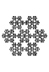
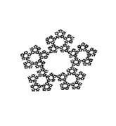
Figure 2. (From left to right) Snowflake, Pentakun

Remark 4.16.

Regarding Examples 4.10–4.15, even if we replace “$\mbox{{\em Aut}}({\mathbb{C}})$” by “$\mbox{{\em Aut}}({\hat{\mathbb{C}}})$”, we obtain similar results by using Lemma 3.29.

As we see in Examples 4.10–4.15 and Remark 4.16, we have many examples to which we can apply Theorem 4.8.

5. Remarks

We finally give a remark.

Remark 5.1.

We can prove similar results to those in sections 3, 4 (especially Theorems 3.12, 3.19, Proposition 3.22, Lemma 3.24, Theorem 4.8) for a family $\{\Phi^{\lambda}\}_{\lambda\in U}=\{\{\varphi_{i}^{\lambda}\}_{i\in I}\}_{\lambda\in U}$ of hyperbolic conformal iterated function systems (CIFSs) on an open subset $V$ of ${\mathbb{R}}^{p}(p\in{\mathbb{N}})$ without the open set condition, where $\varphi_{i}^{\lambda}:V\rightarrow V$ is a contracting conformal map, and $U$ is a bounded open subset of ${\mathbb{R}}^{d},d\geq p.$ For each $\lambda\in U$, we consider the limit set $J(\Phi^{\lambda})$ of $\Phi^{\lambda}.$ In the above setting, the definition of the transversality condition is modified such that the right hand side of (3.1) is replaced by $C_{1}r^{p}$. The definition of the strong transversality condition is modified such that the right hand side of (3.5) is replaced by $C_{1}^{\prime}r^{p-d}.$ If $p=2$ and each $\varphi_{i}^{\lambda}$ is a holomorphic map, then we can define “analytic transversality family” just like Definition 3.21. The number $``2^{\prime\prime}$ (which represents the dimension of the phase space ${\hat{\mathbb{C}}}$) in results of the previous sections are replaced by the number $p.$ These results will be stated and will be proved in the authors’ upcoming paper [42].

References

[1] L. V. Ahlfors, Complex Analysis 3rd ed.,
International Series in Pure and Applied Mathematics. McGraw-Hill Book Co., New York, 1978.
[2] A. Beardon,
Iteration of Rational Functions,
Graduate Texts in Mathematics 132, Springer-Verlag, 1991.
[3] R. Brück, M. Büger and
S. Reitz, Random iterations of polynomials of the
form : Connectedness of Julia sets, Ergodic Theory Dynam. Systems, 19, (1999), No.5, 1221–1231.
[4] K. Falconer,
Fractal Geometry. Mathematical Foundations and Applications, 2nd edition,
John Wiley & Sons, 2003.
[5] K. Falconer,
Techniques in Fractal Geometry,
John Wiley & Sons, 1997.
[6] J. E. Fornaess and N. Sibony, Random iterations of rational functions, Ergodic Theory Dynam. Systems 11(1991), 687–708.
[7] Z. Gong, W. Qiu and Y. Li,
Connectedness of Julia sets for a quadratic random
dynamical system, Ergodic Theory Dynam. Systems (2003), 23,
1807-1815.
[8] A. Hinkkanen and G. J. Martin,
The dynamics of semigroups of rational functions I,
Proc. London Math. Soc. (3) 73 (1996) 358-384.
[9] J. Kigami,
Analysis on Fractals,
Cambridge Tracts in Math., vol. 143, Cambridge University Press, 2001.
[10] P. Mattila,
Geometry of Sets and Measures in Euclidean spaces,
C. U. P. Cambridge, 1995.
[11] D. Mauldin and M. Urbański,
Graph Directed Markov Systems: Geometry and Dynamics of
Limit Sets, Cambridge University Press, 2003.
[12] V. Mayer, B. Skorulski and M. Urbański, Random
Distance Expanding Mappings, Thermodynamic Formalism, Gibbs
Measures, and Fractal Geometry, Lecture Notes in Math. 2036, Springer
(2011).
[13] E. Mihailescu and M. Urbański,
Transversal families of hyperbolic skew products,
Discrete and Continuous Dynamical Systems Ser. A., 21,
2008, No. 3, 907-928.
[14] J. Milnor,
Dynamics in One Complex Variable (Third Edition),
Annals of Mathematical Studies, Number 160, Princeton University
Press, 2006.
[15] Y. Peres, K. Simon, B. Solomyak,
Absolute continuity for random iterated function systems with overlaps,
J. London Math. Soc. (2) 74, (2006), No. 3, 739-756.
[16] Y. Peres and B. Solomyak,
Absolute continuity of Bernoulli convolution, a simple proof,
Math. Res. Lett., 3, 1996, No. 2, 231-239.
[17] M. Pollicott and K. Simon,
The Hausdorff dimension of -expansions with deleted digits,
Trans. Amer. Math. Soc., 347:3 (1995), 967–983.
[18] F. Przytycki, M. Urbański, Conformal Fractals:
Ergodic Theory Methods, London Mathematical Society Lecture Note Series 371, Cambridge Univ. Press, 2010.
[19] M. Rams, Generic behavior of iterated function systems with overlaps,
Pacific J. Math., Vol. 218, No. 1, 2005, 173–186.
[20] K. Simon, B. Solomyak, and M. Urbański,
Hausdorff dimension of limit sets for parabolic IFS with overlaps,
Pacific J. Math., Vol. 201, No. 2, 2001, 441–478.
[21] B. Solomyak and M. Urbański,
densities for Measures Associated with
Parabolic IFS with Overlaps,
Indiana Univ. Math. J., Vol. 50, No. 4, (2001), 1845–1866.
[22] R. Stankewitz,
Density of repelling fixed points in the Julia set of a rational or entire semigroup II,
Discrete and Continuous Dynamical Systems Ser. A.,
32, (2012), No. 7, 2583-2589.
[23] R. Stankewitz and H. Sumi,
Dynamical properties and structure of Julia sets of postcritically
bounded polynomial semigroups,
Trans. Amer. Math. Soc., 363 (2011), 5293–5319.
[24] H. Sumi,
On dynamics of hyperbolic rational semigroups,
J. Math. Kyoto Univ., Vol. 37, No. 4, 1997, 717–733.
[25]
H. Sumi, On Hausdorff dimension of Julia sets of hyperbolic
rational semigroups,
Kodai Mathematical Journal, 21, (1), 1998, 10-28.
[26] H. Sumi,
Skew product maps related to finitely generated rational semigroups,
Nonlinearity 13 (2000) pp 995-1019.
[27] H. Sumi,
Dynamics of sub-hyperbolic and semi-hyperbolic rational
semigroups and skew products,
Ergodic Theory Dynam. Systems,
(2001), 21, 563-603.
[28] H. Sumi,
Dimensions of Julia sets of expanding rational semigroups,
Kodai Mathematical Journal, Vol. 28, No.2, 2005,
pp390–422. (See also
http://arxiv.org/abs/math.DS/0405522.)
[29] H. Sumi,
Semi-hyperbolic fibered rational maps and rational semigroups,
Ergodic Theory Dynam. Systems, (2006), 26, 893-922.
[30] H. Sumi,
Random dynamics of polynomials and devil’s-staircase-like
functions in the complex plane,
Applied Mathematics and Computation 187 (2007) 489-500
(Proceedings paper).
[31] H. Sumi,
Dynamics of postcritically bounded polynomial semigroups I: connected components of the Julia sets,
Discrete Contin. Dyn. Sys. Ser. A, Vol. 29, No. 3, 2011, 1205–1244.
[32] H. Sumi,
Dynamics of postcritically bounded polynomial semigroups III:
classification of semi-hyperbolic semigroups and random Julia sets which are Jordan curves but not quasicircles,
Ergodic Theory Dynam. Systems, (2010), 30, No. 6, 1869–1902.
[33] H. Sumi,
Interaction cohomology of forward or backward self-similar systems,
Adv. Math., 222, No. 3, (2009) 729–781.
[34] H. Sumi,
Random complex dynamics and semigroups of holomorphic maps,
Proc. London Math. Soc. (2011), 102 (1), 50–112.
[35] H. Sumi,
Rational semigroups, random complex dynamics and singular functions on the complex plane,
survey article, Selected Papers on Analysis and Differential Equations,
Amer. Math. Soc. Transl. (2) Vol. 230, 2010, 161–200.
[36] H. Sumi,
Cooperation principle, stability and bifurcation in random complex dynamics,
preprint 2010, http://arxiv.org/abs/1008.3995.
[37] H. Sumi,
Random complex dynamics and devil’s coliseums,
preprint 2011,
http://arxiv.org/abs/1104.3640.
[38] H. Sumi,
Dynamics of postcritically bounded polynomial semigroups II: fiberwise dynamics and the Julia sets,
preprint, http://arxiv.org/abs/1007.0613.
[39] H. Sumi and M. Urbański,
Measures and dimensions of Julia sets of semi-hyperbolic rational semigroups,
Discrete and Continuous Dynamical Systems Ser. A,
Vol 30, No. 1, 2011, 313–363.
[40] H. Sumi and M. Urbański,
Real Analyticity of Hausdorff Dimension for Expanding
Rational Semigroups,
Ergodic Theory Dynam. Systems,
2010, Vol. 30, No. 2, 601-633.
[41] H. Sumi and M. Urbański,
Bowen parameter and Hausdorff dimension for expanding rational semigroups,
Discrete and Continuous Dynamical Systems Ser. A, 32 (2012), No. 7, 2591-2606.
[42] H. Sumi and M. Urbański, in preparation.
[43] A. Zdunik,
Parabolic orbifolds and the dimension of the maximal measure for rational maps,
Invent. Math. 99 (1990), no. 3, 627–649.
[44]
W. Zhou and F. Ren,
The Julia sets of the random iteration of rational functions,
Chinese Sci. Bull., 37 (12), 1992, p969-971.