A Variational Bayesian Method to Inverse Problems with Impulsive Noise

Abstract

We propose a novel numerical method for solving inverse problems subject to impulsive noises which possibly contain a large number of outliers. The approach is of Bayesian type, and it exploits a heavy-tailed $t$ distribution for data noise to achieve robustness with respect to outliers. A hierarchical model with all hyper-parameters automatically determined from the given data is described. An algorithm of variational type by minimizing the Kullback-Leibler divergence between the true posteriori distribution and a separable approximation is developed. The numerical method is illustrated on several one- and two-dimensional linear and nonlinear inverse problems arising from heat conduction, including estimating boundary temperature, heat flux and heat transfer coefficient. The results show its robustness to outliers and the fast and steady convergence of the algorithm.
key words: impulsive noise, robust Bayesian, variational method, inverse problems

1 Introduction

We are interested in Bayesian approaches for inverse problems subject to impulsive noises. Bayesian inference provides a principled framework for solving diverse inverse problems, and has demonstrated distinct features over deterministic techniques, e.g., Tikhonov regularization. Firstly, it can yield an ensemble of plausible solutions consistent with the given data. This enables quantifying the uncertainty of a specific solution, e.g., with credible intervals. In contrast, deterministic techniques generally content with singling out one solution from the ensemble. Secondly, it provides a flexible regularization since hierarchical modeling can partially resolve the nontrivial issue of choosing an appropriate regularization parameter. It is known that the underlying mechanism is balancing principle [22]. Thirdly, it allows seamlessly integrating structural/multiscale features of the problem through careful prior modeling. Therefore, it has attracted attention in a wide variety of applied disciplines, e.g., geophysics [37, 34], medical imaging [18, 27, 1] and heat conduction [13, 39, 40, 14], see also [32, 28, 30, 31] for other applications. For an overview of methodological developments, we refer to the monographs [37, 26].

Amongst existing studies on Bayesian inference for inverse problems, the Gaussian noise model has played a predominant role. This is often justified by appealing to central limit theorem. The theorem asserts that the normal distribution is a suitable model for data that are formed as the sum of a large number of independent components. Even in the absence of such justifications, this model is still preferred due to its computational/analytical conveniences, i.e., it allows direct computation of the posterior mean and variance and easy exploration of the posterior state space (for linear models with Gaussian priors). A well acknowledged limitation of the Gaussian model is its lack of robustness against the outliers, i.e., data points that lie far away from the bulk of the data, in the observations: A single aberrant data point can significantly influence all the parameters in the model, even for these with little substantive connection to the outlying observations [16, pp. 443].

However, it is clear that not all real-world data can be adequately described by the Gaussian model. For example, Laplacian noises can arise when acquiring certain signals [2], and salt-and-pepper noises are very common in natural images/signals due to faulty memory location and transmission in noisy channels [6]. The impulsive nature of these noises is reflected by the heavy tail of their distributions and thus the presence of, possibly of a significant amount, outliers in the data. Physically, such noises arise from uncertainties in instrument calibration, physical limitations of acquisition devices and experimental (operation) conditions. Due to its lack of robustness, an inadvertent adoption of the Gaussian model can seriously compromise the accuracy of the estimate, and consequently does not allow full extraction of the information provided by the data.

This calls for methods that are robust to the presence of outliers. There are several ways to derive robust estimates. One classical approach is to first identify the outliers with noise detectors, e.g., by adaptive media filter, and then to perform inversion/reconstruction on the data set with outliers excluded [16, 6]. The success of such procedures relies crucially on the reliability of the noise detector. However, it can be highly nontrivial to accurately identify all outliers, especially in high dimensions, and mis-identification can adversely affect the quality of subsequent inversion. This necessitates developing systematic strategies for handling impulsive noises, which can be achieved by modeling the outliers explicitly with a heavy-tailed noise distribution. The Student’s $t$ and Laplace distributions are two most popular choices. The use of the $t$-distribution in robust Bayesian analysis is well recognized, see [29] for its usage in statistical contexts. In [12], the application of the EM algorithm to $t$ models was shown. Recently, Tipping and Lawrence [38] developed a robust Bayesian interpolation with the $t$-distribution. Alternatively, the Laplace distribution may be employed, see, e.g., [15] for robust probabilistic principal component analysis.

This paper studies the potentials of one robust Bayesian formulation for inverse problems subject to impulsive noises. Impulsive noise has received some recent attention in deterministic inversion, see [10, 9] and references therein, but not in the Bayesian framework. The salient features of the proposed approach include uncertainty quantification of the computed solution, robustness to data outliers, and general applicability to both linear and nonlinear inverse problems. Therefore, it complements the developments of robust formulations in the framework of deterministic inverse problems [10, 9]. As to the numerical exploration of the Bayesian model, we capitalize on the variational method developed in machine learning [25, 3, 4] for approximate inference, and thus achieve reasonable computational efficiency. The application of variational Bayesian formulations to inverse problems, especially nonlinear ones, is of relatively recent origin [35, 23], and their robust counterparts seem largely unexplored.

The rest of the paper is structured as follows. A hierarchical formulation based on the $t$ distribution for the noise is derived in Section 2. The variational method for numerically exploring the posterior is described in Section 3, and two algorithms are developed for linear and nonlinear inverse problems, respectively. In Section 4, numerical results for four benchmark inverse problems arising in heat transfer are presented to illustrate the features of the formulation and the convergence behavior of the algorithms.

2 Hierarchical Bayesian inference

In this section, we formulate the hierarchical Bayesian model for inverse problems subject to impulsive noises. The focus is on the noise model and hyper-parameter treatment.

We consider for the following finite-dimensional linear inverse problem

$$\mathbf{K(u)}=\mathbf{y},$$ (1)

where $\mathbf{K}:\mathbb{R}^{m}\to\mathbb{R}^{n}$, $\mathbf{u}\in\mathbb{R}^{m}$ and $\mathbf{y}\in\mathbb{R}^{n}$ represent the (possibly nonlinear) forward model, the sought-for solution and noisy observational data, respectively.

In Bayesian formalism, the likelihood function $p(\mathbf{y}|\mathbf{u})$ incorporates the information contained in the data $\mathbf{y}$, and it is dictated by the noise model. Let the given data $\mathbf{y}$ be subjected to additive noises, i.e.,

$$\mathbf{y}=\mathbf{y}^{\dagger}+\boldsymbol{\zeta},$$

where $\boldsymbol{\zeta}\in\mathbb{R}^{n}$ is a random vector corrupting the exact data $\mathbf{y}^{\dagger}$. In practice, a Gaussian distribution on each component $\zeta_{i}$ is customarily assumed. The validity of this assumption relies crucially on being not heavy-tailed and the symmetry of the distribution, and the violation of either condition may render the resulting Bayesian model invalid and inappropriate, which may seriously compromise the accuracy of the posteriori estimate.

In practice, data outliers can arise due to, e.g., erroneous recording and transmission in noisy channels, which makes the Gaussian model unsuitable. Following the interesting works [29, 17, 38], we choose to model the outliers explicitly by a heavy-tailed distribution, and this yields a seamless and systematic framework for treating impulsive noises. We focus on the $t$ model [16], where the noises $\zeta_{i}$ are independent and identically distributed according to a centered $t$ distribution, i.e.,

$$p(\zeta_{i};\nu,\sigma)=\frac{\Gamma(\frac{\nu+1}{2})}{\Gamma(\frac{\nu}{2})\sqrt{\pi\nu}\sigma}\left\{1+\frac{1}{\nu}\left(\frac{\zeta_{i}}{\sigma}\right)^{2}\right\}^{-\frac{\nu+1}{2}},$$

where $\nu$ is a degree of freedom parameter, $\sigma$ is a scale parameter [16], and $\Gamma(\cdot)$ is the standard Gamma function. Consequently, the likelihood function $p(\mathbf{y}|\mathbf{u})$ is given by

$$p(\mathbf{y}|\mathbf{u})=\left(\frac{\Gamma(\frac{\nu+1}{2})}{\Gamma(\frac{\nu}{2})\sqrt{\pi\nu}\sigma}\right)^{n}\prod_{i=1}^{n}\left\{1+\frac{1}{\nu}\left(\frac{|(\mathbf{K(u)-y})_{i}|}{\sigma}\right)^{2}\right\}^{-\frac{\nu+1}{2}},$$ (2)

where the subscript $i$ denotes the $i$th entry of a vector.

In Bayesian formalism, structural prior knowledge about the unknown $\mathbf{u}$ is encoded in the prior distribution $p(\mathbf{u})$. Here we focus on the following simple random field

$$p(\mathbf{u}|\lambda)=C\lambda^{\frac{s}{2}}\exp\left(-\frac{\lambda}{2}\|\mathbf{Lu}\|_{2}^{2}\right),$$ (3)

where $\|\cdot\|_{2}$ denotes the Euclidean norm and $C$ is a normalizing constant. The matrix $\mathbf{L}\in\mathbb{R}^{s\times m}$, whose rank is $s$, encodes the structural interactions between neighboring sites, and $\lambda$ is a scaling parameter.

The hyper-parameters $\nu$, $\sigma$ and $\lambda$ in the likelihood $p(\mathbf{y}|\mathbf{u})$ and the prior $p(\mathbf{u}|\lambda)$ play the crucial role of regularization parameters in classical regularization [22]. Bayesian formalism resolves the issue through hierarchical modeling and determines them automatically from the data $\mathbf{y}$. A standard practice to select priors for hyper-parameters is to use conjugate priors. For the parameter $\lambda$, the conjugate prior is a Gamma distribution $G(t;\alpha,\beta)$, which is defined by

$$G(t;\alpha,\beta)=\frac{\beta^{\alpha}}{\Gamma(\alpha)}t^{\alpha-1}e^{-\beta t},$$ (4)

where $\alpha$ and $\beta$ are nonnegative constants. The parameters $\nu$ and $\sigma$ do not admit easy conjugate form, and one may opt for the maximum likelihood approach when appropriate.

According to Bayes’ rule, the posterior $p(\mathbf{u},\lambda|\mathbf{y})$ is related to the data $\mathbf{y}$ by

$$p(\mathbf{u},\lambda|\mathbf{y})=\frac{p(\mathbf{y}|\mathbf{u})p(\mathbf{u}|\lambda)p(\lambda)}{\int\int p(\mathbf{y}|\mathbf{u})p(\mathbf{u}|\lambda)p(\lambda)d\mathbf{u}d\lambda}.$$

Upon ignoring the (unimportant) normalizing constant $p(\mathbf{y})=\int\int p(\mathbf{y}|\mathbf{u})p(\mathbf{u}|\lambda)p(\lambda)d\mathbf{u}d\lambda$, the posterior $p(\mathbf{u},\lambda|\mathbf{y})$ may be simply evaluated as

$$p(\mathbf{u},\lambda|\textbf{y})\propto\left(\frac{\Gamma(\frac{\nu+1}{2})}{\Gamma(\frac{\nu}{2})\sqrt{\pi\nu}\sigma}\right)^{n}\prod_{i=1}^{n}\left\{1+\frac{1}{\nu}\left(\frac{|(\mathbf{K(u)-y})_{i}|}{\sigma}\right)^{2}\right\}^{-\frac{\nu+1}{2}}\cdot\lambda^{\frac{s}{2}}e^{-\frac{\lambda}{2}\|\mathbf{Lu}\|_{2}^{2}}\cdot\lambda^{\alpha_{0}-1}e^{-\beta_{0}\lambda},$$ (5)

where $(\alpha_{0},\beta_{0})$ is the parameter pair of the Gamma distribution for $\lambda$.

The posterior state space $p(\mathbf{u},\lambda|\mathbf{y})$ is often high dimensional, and thus it can only be numerically explored. In Section 3, we shall develop an efficient variational method for its approximate inference.

3 Variational approximation

In this section, we describe a variational method for efficiently constructing an approximation to the posterior distribution (5). It can deliver point estimates together with uncertainties for both the solution $\mathbf{u}$ and the hyper-parameter $\lambda$. There are three major obstacles in getting a faithful approximation:

• nongaussian likelihood ($t$ instead of Gaussian distribution),

• statistical dependency between $\mathbf{u}$ and $\lambda$, and

• possible nonlinearity of the forward mapping $\mathbf{K}$.

To circumvent these obstacles, we shall make use of three ideas: scale-mixture representation of the $t$ distribution, variational (separable) approximation for decoupling dependency, and recursive linearization for resolving nonlinearity.

First we describe the scale-mixture representation. In the posterior (5), the $t$ likelihood makes it hard to find or define a good approximation. Fortunately, it can be represented as follows [16, pp. 446]

$$p(\zeta_{i}|\nu,\sigma) =\frac{\Gamma(\frac{\nu+1}{2})}{\Gamma(\frac{\nu}{2})\sqrt{\pi\nu}\sigma}\left\{1+\frac{1}{\nu}\left(\frac{\zeta_{i}}{\sigma}\right)^{2}\right\}^{-\frac{\nu+1}{2}}$$

$$=\int_{0}^{\infty}\sqrt{\frac{w_{i}}{2\pi}}e^{-\frac{w_{i}}{2}\zeta_{i}^{2}}p(w_{i};\nu,\sigma)dw_{i},$$

where the density $p(w_{i})$ is given by $p(w_{i};\nu,\sigma)=\frac{(\frac{\nu\sigma^{2}}{2})^{\frac{\nu}{2}}}{\Gamma(\frac{\nu}{2})}w^{\frac{\nu}{2}-1}e^{-\frac{\nu\sigma^{2}}{2}w}=G\left(w_{i};\tfrac{\nu}{2},\tfrac{\nu\sigma^{2}}{2}\right)$, c.f. (4). To simplify the expression, we introduce two independent variables $\alpha_{1}$ and $\beta_{1}$ by

$$\alpha_{1}=\frac{\nu}{2}\quad\mbox{and}\quad\beta_{1}=\frac{\nu\sigma^{2}}{2},$$

and work with the parameters $\alpha_{1}$ and $\beta_{1}$ hereon. Then we have the following succinct formula

$$p(\zeta_{i}|\alpha_{1},\beta_{1})=\int_{0}^{\infty}\sqrt{\frac{w_{i}}{2\pi}}e^{-\frac{w_{i}}{2}\zeta_{i}^{2}}p(w_{i};\alpha_{1},\beta_{1})dw_{i},$$

with $p(w_{i};\alpha_{1},\beta_{1})=G\left(w_{i};\alpha_{1},\beta_{1}\right)$. Therefore, the $t$ model is a mixture (average) of an infinite number of Gaussians of varying precisions $w_{i}$, with the mixture weight $w_{i}$ specified by the Gamma distribution $p(w_{i};\alpha_{1},\beta_{1})$. The representation also explains its heavy tail: for small $w_{i}$, the random variable $\zeta_{i}$ follow a Gaussian distribution with a large variance, and thus the realizations are likely to take large values, which behaves more or less like outliers. By means of scale mixture, we have introduced an extra variable, but effectively converted a $t$ distribution into a Gaussian distribution. In sum, we have arrived at the following augmented posterior

$$p(\mathbf{u},\mathbf{w},\lambda|\mathbf{y})\propto|\mathbf{W}|^{\frac{1}{2}}e^{-\frac{1}{2}\|\mathbf{K(u)}-\mathbf{y}\|_{\mathbf{W}}^{2}}\cdot p(\mathbf{w};\alpha_{1},\beta_{1})\cdot\lambda^{\frac{s}{2}}e^{-\frac{\lambda}{2}\|\mathbf{Lu}\|_{2}^{2}}\cdot\lambda^{\alpha_{0}-1}e^{-\beta_{0}\lambda},$$ (6)

where $\mathbf{w}\in\mathbb{R}^{n}$ is an auxiliary random vector following the Gamma distribution, i.e.,

$$p(\mathbf{w};\alpha_{1},\beta_{1})=\prod_{i=1}^{n}G(w_{i};\alpha_{1},\beta_{1})=G(\mathbf{w};\alpha_{1},\beta_{1}),$$

$\mathbf{W}$ is a diagonal matrix with diagonal $\mathbf{w}$, and the weighted norm $\|\cdot\|_{\mathbf{W}}$ is defined by $\|\mathbf{v}\|_{\mathbf{W}}^{2}=\mathbf{v}^{\mathrm{T}}\mathbf{Wv}$. The posterior $p(\mathbf{u},\mathbf{w},\lambda|\mathbf{y})$ is computationally more amenable with the variational method.

Next we describe the variational method for approximately exploring the posterior (6) in case of a linear operator $\mathbf{K}$, i.e., $\mathbf{K}(\mathbf{u})=\mathbf{Ku}$. The derivations here follow closely [23, 38]. An approximation can be derived as follows. One first transforms it into an equivalent optimization problem using the Kullback-Leibler divergence and then obtains an approximation by solving the optimization problem inexactly. The divergence $D_{KL}(q(\mathbf{u},\mathbf{w},\lambda)|p(\mathbf{u},\mathbf{w},\lambda|\mathbf{y}))$ between two densities $q(\mathbf{u},\mathbf{w},\lambda)$ and $p(\mathbf{u},\mathbf{w},\lambda|\mathbf{y})$ is defined by

$$D_{KL}(q(\mathbf{u},\mathbf{w},\lambda)|p(\mathbf{u},\mathbf{w},\lambda|\mathbf{y})) =\int\int\int q(\mathbf{u},\mathbf{w},\lambda)\ln\frac{q(\mathbf{u},\mathbf{w},\lambda)}{p(\mathbf{u},\mathbf{w},\lambda,\mathbf{y})}d\mathbf{u}d\mathbf{w}d\lambda+\log p(\mathbf{y}),$$

where $p(\mathbf{y})$ is a normalizing constant. Since the divergence $D_{KL}$ is nonnegative and vanishes if and only if $q$ coincides with $p$, minimizing $D_{KL}$ effectively transforms the problem into an equivalent optimization problem. We shall minimize the following functional, which is also denoted by $D_{KL}$

$$D_{KL}(q(\mathbf{u},\mathbf{w},\lambda)|p(\mathbf{u},\mathbf{w},\lambda|\mathbf{y}))=\int\int\int q(\mathbf{u},\mathbf{w},\lambda)\ln\frac{q(\mathbf{u},\mathbf{w},\lambda)}{p(\mathbf{u},\mathbf{w},\lambda,\mathbf{y})}d\mathbf{u}d\mathbf{w}d\lambda.$$ (7)

However, directly minimizing $D_{KL}$ is still intractable since the posterior $p(\mathbf{u},\mathbf{w},\lambda|\mathbf{y})$ is not available in closed form. We impose a separability (conditionally independence) condition for the posterior distributions of $\mathbf{u}$, $\mathbf{w}$ and $\lambda$ to arrive at a tractable approximation, i.e.,

$$q(\mathbf{u},\mathbf{w},\lambda)=q(\mathbf{u})q(\mathbf{w})q(\lambda).$$ (8)

Algorithm 1 Variational approximation for linear models $\mathbf{K}$

1:  Set initial guess $q^{0}(\mathbf{w})$ and $q^{0}(\lambda)$;

2:  for $k=1,\dots,K$ do

3:     Find $q^{k}(\mathbf{u})$ by

$$q^{k}(\mathbf{u})=\arg\min_{q(\mathbf{u})}D_{KL}(q(\mathbf{u})q^{k-1}(\mathbf{w})q^{k-1}(\lambda)|p(\mathbf{u},\mathbf{w},\lambda|\mathbf{y}));$$

4:     Find $q^{k}(\mathbf{w})$ by

$$q^{k}(\mathbf{w})=\arg\min_{q(\mathbf{w})}D_{KL}(q^{k}(\mathbf{u})q(\mathbf{w})q^{k-1}(\lambda)|p(\mathbf{u},\mathbf{w},\lambda|\mathbf{y}));$$

5:     Find $q^{k}(\lambda)$ by

$$q^{k}(\lambda)=\arg\min_{q(\lambda)}D_{KL}(q^{k}(\mathbf{u})q^{k}(\mathbf{w})q(\lambda)|p(\mathbf{u},\mathbf{w},\lambda|\mathbf{y}));$$

6:     Check a stopping criterion;

7:  end for

8:  Return approximation $q^{k}(\mathbf{u})q^{k}(\mathbf{w})q^{k}(\lambda)$.

Under condition (8), an approximation can be computed by Algorithm 1. Each step of the algorithm can be further developed as follows. Setting the first variation of $D_{KL}$ with respect to $q(\mathbf{u})$ to zero gives

$$q^{k}(\mathbf{u})\propto\exp\left(E_{q^{k-1}(\mathbf{w})q^{k-1}(\lambda)}[\ln p(\mathbf{u},\mathbf{w},\lambda,\mathbf{y})]\right).$$

It follows that $q^{k}(\mathbf{u})$ follows a Gaussian distribution with covariance $\mathrm{cov}_{q^{k}(\mathbf{u})}$ and mean $\mathbf{u}_{k}$ given by

$$\mbox{cov}_{q^{k}(\mathbf{u})}[\mathbf{u}]=\left[\mathbf{K}^{\mathrm{T}}\mathbf{W}_{k}\mathbf{K}+\lambda_{k}\mathbf{L}^{\mathrm{T}}\mathbf{L}\right]^{-1}\quad\mbox{and}\quad\mathbf{u}_{k}:=E_{q^{k}(\mathbf{u})}[\mathbf{u}]=\mbox{cov}_{q^{k}(\mathbf{u})}[\mathbf{u}]\mathbf{K}^{\mathrm{T}}\mathbf{W}_{k}\mathbf{y},$$

respectively, where $\lambda_{k}=E_{q^{k-1}(\lambda)}[\lambda]$ and $\mathbf{W}_{k}=E_{q^{k-1}(\mathbf{w})}[\mathbf{W}]$, i.e.,

$$q^{k}(\mathbf{u})=N(\mathbf{u};\mathbf{u}_{k},[\mathbf{K}^{\mathrm{T}}\mathbf{W}_{k}\mathbf{K}+\lambda_{k}\mathbf{L}^{\mathrm{T}}\mathbf{L}]^{-1}),$$

where $N$ refers to a normal distribution. Analogously, we can show that $q^{k}(\mathbf{w})$ and $q^{k}(\lambda)$ take a factorized form, i.e.,

$$q^{k}(\mathbf{w}) =G\left(\mathbf{w};\alpha_{1}+\tfrac{1}{2},\beta_{1}+\tfrac{1}{2}E_{q^{k}(\mathbf{u})}[|\mathbf{Ku}-\mathbf{y}|^{2}]\right),$$

$$q^{k}(\lambda) =G\left(\lambda;\alpha_{0}+\tfrac{s}{2},\beta_{0}+\tfrac{1}{2}E_{q^{k}(\mathbf{u})}[\|\mathbf{Lu}\|_{2}^{2}]\right).$$

Thus Steps 4 and 5 involve simply updating their respective parameter pairs.

There are several viable choices for the stopping criterion at Step 6. In practice, the following two heuristics work well. One is to monitor the relative change of the inverse solution $\mathbf{u}_{k}$. If the change between two consecutive iterations falls below a given tolerance $tol$, i.e., $\|\mathbf{u}_{k}-\mathbf{u}_{k-1}\|_{2}/\|\mathbf{u}_{k}\|_{2}\leq tol$, then the algorithm may stop. Another is to monitor the variable $\lambda_{k}$. Numerically, we observe that the algorithm converges reasonably fast and steadily.

We briefly remark on the choice of the pair $(\alpha_{1},\beta_{1})$. For our experiments in Section 4, one fixed pair $(\alpha_{1},\beta_{1})=(1,1\times 10^{-10})$ works fairly well. In principle, it is plausible to estimate them from the data simultaneously with other parameters in order to adaptively accommodate noise features, especially for large data sets [16]. However, there are no conjugate priors compatible with the adopted variational framework [38]. Therefore, one possible way is to maximize the divergence with respect to $(\alpha_{1},\beta_{1})$. It is easy to find that in (7), the only term relates to $\alpha_{1}$ and $\beta_{1}$ is given by

$$n\alpha_{1}\ln\beta_{1}-n\ln\Gamma(\alpha_{1})+(\alpha_{1}-1)\sum_{i=1}^{n}E_{q^{\ast}(w_{i})}[\ln w_{i}]-\beta_{1}\sum_{i=1}^{n}E_{q^{\ast}(w_{i})}[w_{i}].$$

Taking derivatives with respect to $\alpha_{1}$ and $\beta_{1}$, we arrive at

$$\ln\beta_{1}-\psi(\alpha_{1})+\frac{1}{n}\sum_{i=1}^{n}E_{q^{\ast}(w_{i})}[\ln w_{i}]=0,$$

$$\frac{\alpha_{1}}{\beta_{1}}-\frac{1}{n}\sum_{i=1}^{n}E_{q^{\ast}(w_{i})}[w_{i}]=0,$$

where $\psi(s)=\frac{\partial}{\partial s}\ln\Gamma(s)$ denotes the digamma function. The solution to the system is not available in closed form, but upon eliminating the variable $\beta_{1}$, it can be solved efficiently by the Newton-Raphson method, see e.g., [8, Sect. 3.1].

Finally, we briefly mention the extension to nonlinear problems via recursive linearization [7, 23]. The main idea is to approximate the nonlinear model $\mathbf{K}(\mathbf{u})$ by its first-order Taylor expansion $\widetilde{\mathbf{K}}(\mathbf{u})$ around the mode $\tilde{\mathbf{u}}$ of an approximate posterior, i.e.,

$$\widetilde{\mathbf{K}}(\mathbf{u})=\mathbf{K}(\tilde{\mathbf{u}})+\mathbf{J}(\mathbf{u}-\tilde{\mathbf{u}}),$$

where $\mathbf{J}=\nabla_{\mathbf{u}}\mathbf{K(\tilde{\mathbf{u}})}$ is the Jacobian of the model $\mathbf{K}$ with respect to $\mathbf{u}$. With this linearized model $\widetilde{\mathbf{K}}(\mathbf{u})$ in place of $\mathbf{K}(\mathbf{u})$, Algorithm 1 might be employed to deliver an approximation. The mode of the this newly-derived approximation is then taken for (hopefully) more accurately capturing the nonlinearity of the genuine model $\mathbf{K}(\mathbf{u})$. This procedure is repeated until a satisfactory solution is achieved, which gives rise to Algorithm 2. In the inner loop, the variational approximation needs not be carried out very accurately. As to the stopping criterion at Step 7, there are several choices, e.g., based on the relative change of the inverse solution $\mathbf{u}$.

Algorithm 2 Variational approximation for nonlinear models $\mathbf{K}$

1:  Given initial guess $q^{0}(\mathbf{u})$, $q^{0}(\mathbf{w})$ and $q^{0}(\lambda)$, and set $k=0$.

2:  repeat

3:     Calculate the mode $\tilde{\mathbf{u}}^{k}$ and the Jacobian $\mathbf{J}^{k}=\nabla_{\mathbf{u}}\mathbf{K}(\tilde{\mathbf{u}}^{k})$.

4:     Construct the linearized model, i.e. $\widetilde{\mathbf{K}}(\mathbf{u})=\mathbf{K}(\tilde{\mathbf{u}}^{k})+\mathbf{J}^{k}(\mathbf{u}-\tilde{\mathbf{u}}^{k})$;

5:     Find a variational approximation $q^{k+1}(\mathbf{u})q^{k+1}(\mathbf{w})q^{k+1}(\lambda)$ using $\widetilde{\mathbf{K}}(\mathbf{u})$ by Algorithm 1;

6:     Set $k=k+1$;

7:  until A stopping criterion is satisfied

8:  Return $q^{k}(\mathbf{u})q^{k}(\mathbf{w})q^{k}(\lambda)$ as the solution.

4 Numerical experiments

Now we illustrate the proposed method on several benchmark inverse problems in 1d and 2d heat transfer. These examples are adapted from literature [36, 20, 23, 39, 24], and include both linear and nonlinear models. Throughout, the noisy data $\mathbf{y}$ are generated as follows

$$y_{i}=\left\{\begin{array}[]{ll}y_{i}^{\dagger},&\mbox{with probability }1-r\\ y_{i}^{\dagger}+\epsilon\zeta_{i},&\mbox{with probability }r\end{array}\right.$$

where $\zeta_{i}$ follow the standard normal distribution, and $(\epsilon,r)$ control the noise pattern: $r$ is the corruption percentage and $\epsilon=\max_{i}\{|y_{i}^{\dagger}|\}$ is the corruption magnitude. The matrix $\mathbf{L}$ in the prior $p(\mathbf{u}|\lambda)$ is taken to be the first-order finite-difference operator, which enforces smoothness on the sought-for solution $\mathbf{u}$. The parameter pairs $(\alpha_{0},\beta_{0})$ and $(\alpha_{1},\beta_{1})$ are both set to $(1.0,1.0\times 10^{-10})$. We have also experimented with updating $(\alpha_{1},\beta_{1})$, but it brings little improvement. Hence, we refrain from presenting the results by adaptively updating $(\alpha_{1},\beta_{1})$. We shall measure the accuracy of a solution $\mathbf{u}$ by the relative error

$$e=\|\mathbf{u}-\mathbf{u}^{\dagger}\|_{2}/\|\mathbf{u}^{\dagger}\|_{2}.$$

The algorithm is terminated if the relative change of $\mathbf{u}$ falls below $tol=1.0\times 10^{-5}$. All the computations were performed on a dual core personal computer with 1.00 GB RAM with MATLAB version 7.0.1 .

4.1 Cauchy problem

This example is taken from [23, Sect. 5.2.1]. Here we consider the Cauchy problem for steady state heat conduction. Let $\Omega$ be the unit square $(0,1)^{2}$ with its boundary $\Gamma$ divided into two disjoint parts, i.e., $\Gamma_{i}=[0,1]\times\{1\}$ and $\Gamma_{c}=\Gamma\backslash\Gamma_{i}$. The steady-state heat conduction is described by

$$-\Delta y=0\quad\mbox{in }\Omega.$$

It is subjected to the boundary conditions

$$\frac{\partial y}{\partial n}=g\quad\mbox{on}\quad\Gamma_{c}\quad\quad\mbox{and}\quad\quad y=u\quad\mbox{on}\quad\Gamma_{i},$$

where $n$ denotes the unit outward normal. The linear operator $K$ maps $u$ (with $g=0$) to $y$ restricted to the segments $\Gamma_{o}=\{0,1\}\times(0,1)\subset\Gamma_{c}$. We refer to Fig. 1(a) for a schematic plot of the domain and its boundaries. The inverse problem seeks the unknown $u$ from noisy data $y$. It arises, e.g., in the study of re-entrant space shuttles [5] and electro-cardiography [11]. For the inversion, the solution $y$ is given by $\sin\pi x_{1}e^{\pi x_{2}}+x_{1}+x_{2}$, from which both $g$ and $u$ can be evaluated directly. The operator $K$ is discretized using piecewise linear finite element with $3200$ triangular elements, see [23, 24] for details. The number of measurements $\mathbf{y}$ is $80$, and the unknown $\mathbf{u}$ is of dimension $41$.

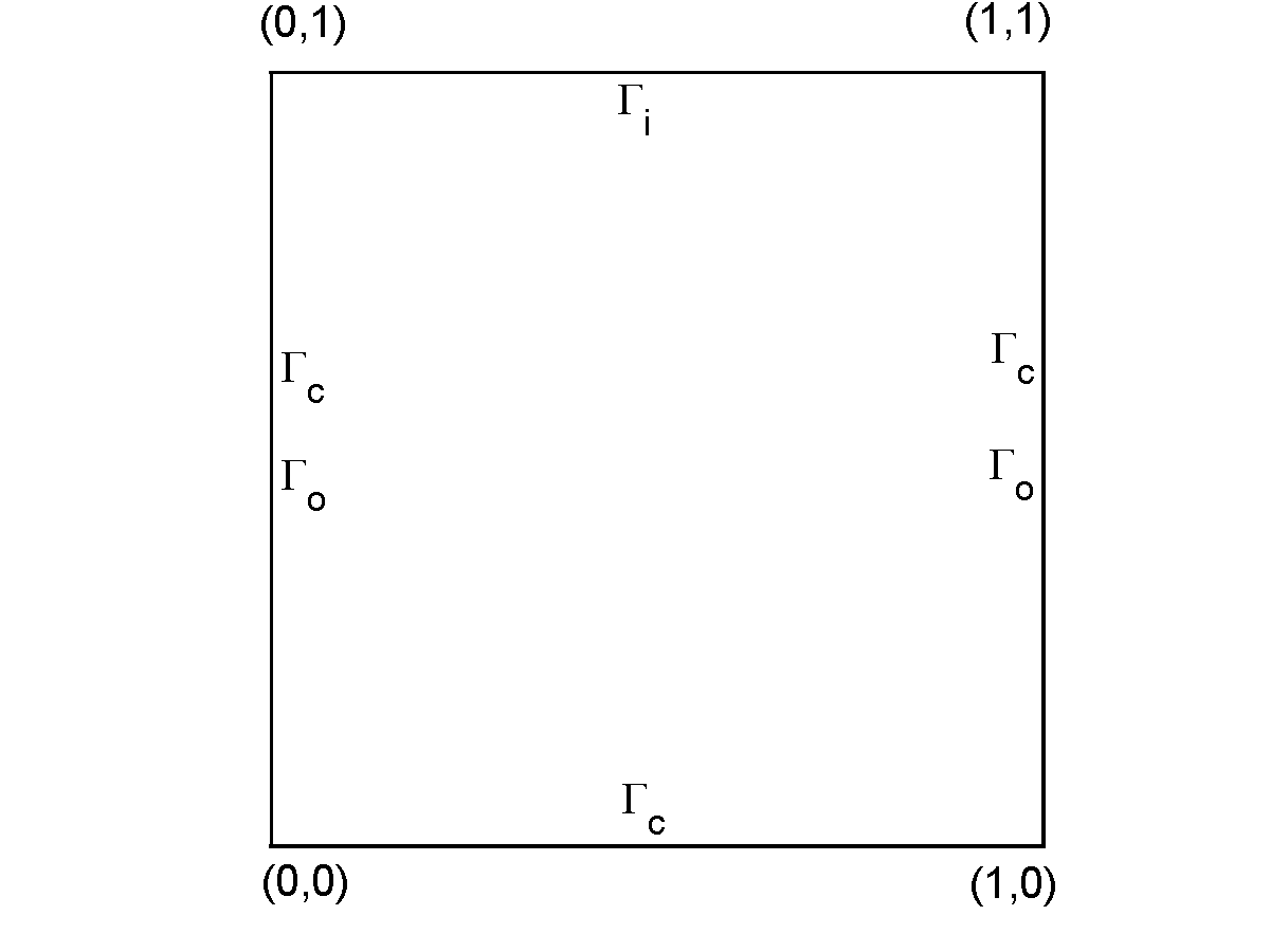
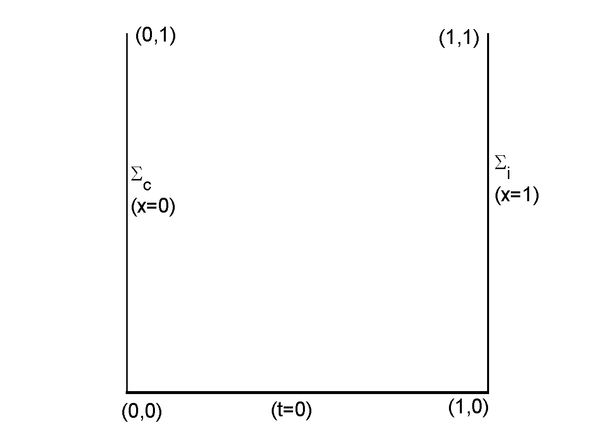
(a)	(b)

Figure 1: The domain and boundaries for Example 1 (a) and Example 3 (b).

The numerical results for the example with various levels of noises are shown in Table 1, where $e$ refers to the relative error. A first observation is that the corruption percentage $r$ plays an important role in the error $e$, and there is a sudden loss of the accuracy $e$ as $r$ increases from $0.4$ to $0.5$. Nonetheless, the reconstruction remains very accurate for $r$ up to $0.9$.

Table 1: Numerical results for Example 1 with various noise levels.

$r$	$0.1$	$0.2$	$0.3$	$0.4$	$0.5$	$0.6$	$0.7$	$0.8$	$0.9$
$\lambda$	8.56e-1	8.51e-1	8.49e-1	8.49e-1	8.36e-1	8.28e-1	8.28e-1	8.28e-1	8.27e-1
$e$	2.33e-4	3.67e-4	3.65e-4	3.67e-4	1.59e-3	2.49e-3	2.49e-3	2.49e-3	2.53e-3

A typical realization of the noisy data of level $r=0.5$ is shown in Fig. 2(a). We observe that some data points deviate significantly from the exact ones, and are completely erroneous. The solutions (mean of the Bayesian solution) by the proposed approach ($t$ model) and the Gaussian model is shown in Figs. 2(b) and 2(d), respectively, where $x_{1}$ is the first spatial coordinate. Here, for the Gaussian model, the regularization parameter $\eta$ is manually tuned, i.e. $\eta=4.64$, so as to yield a solution with the smallest possible error. The solution by the $t$ model is in excellent agreement with the exact one, while that by the standard approach is completely off the track. This shows clearly the robustness of the $t$ model. The covariance, see Fig. 2(c), can be used for quantifying the uncertainty of a specific solution. The covariance is relatively smooth, and decays quickly away from neighboring sites. The weight $\mathbf{w}$ admits nice interpretations. We plot in Fig. 2(e) the noise (solid line, value in blue) and the weight (dashed line, value in green). There is a one-to-one correspondence of the noise sites and the sites of the weight with small values. Thus the weight $\mathbf{w}$ can accurately detect the locations of the noises and effectively prunes out the noises from the inversion procedure simultaneously. The convergence of Algorithm 1 is very steady and fast, see Fig. 2(f), and it is reached within about ten iterations. The convergence of the scalar $\lambda$ seems monotonic.

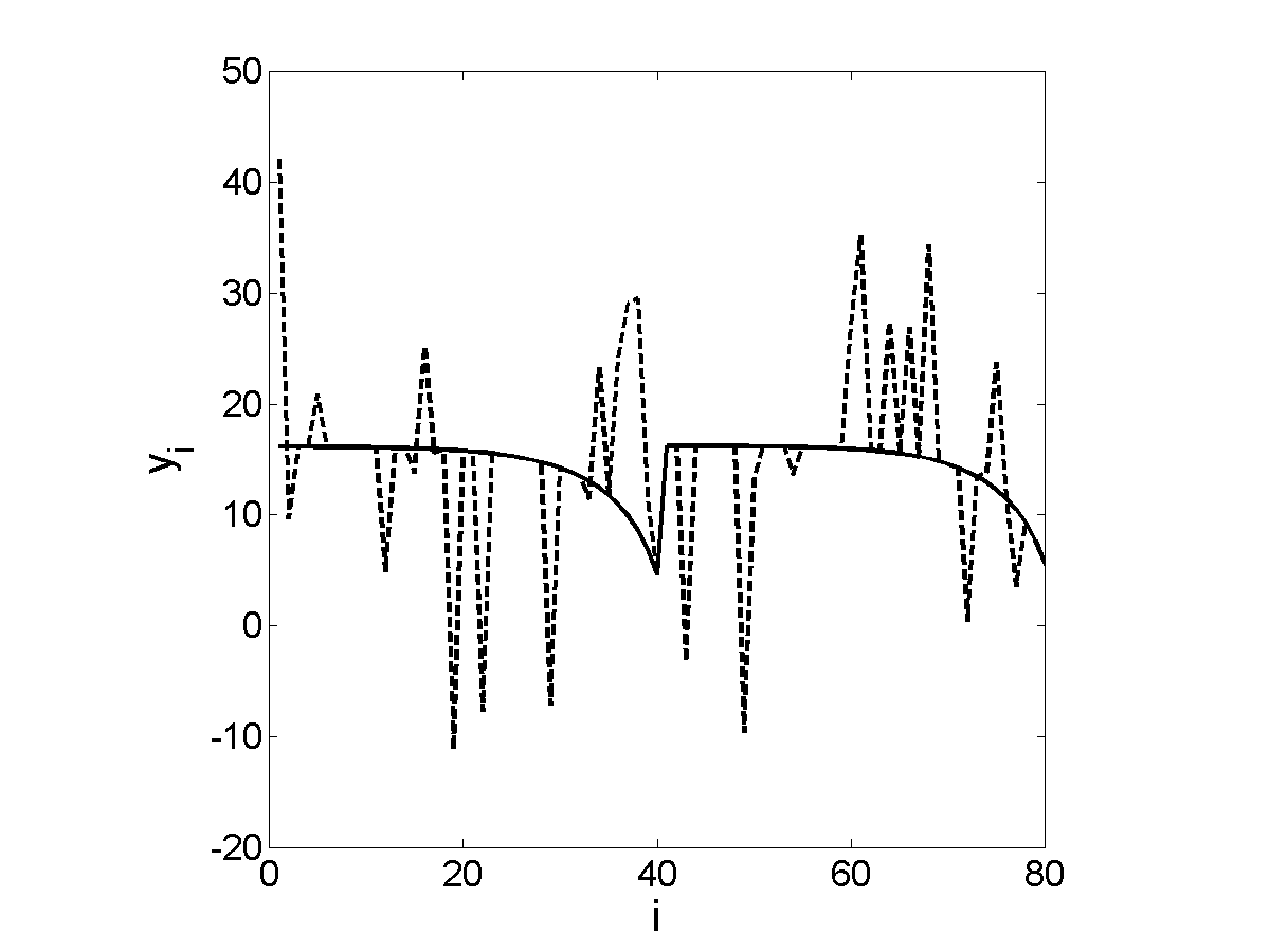
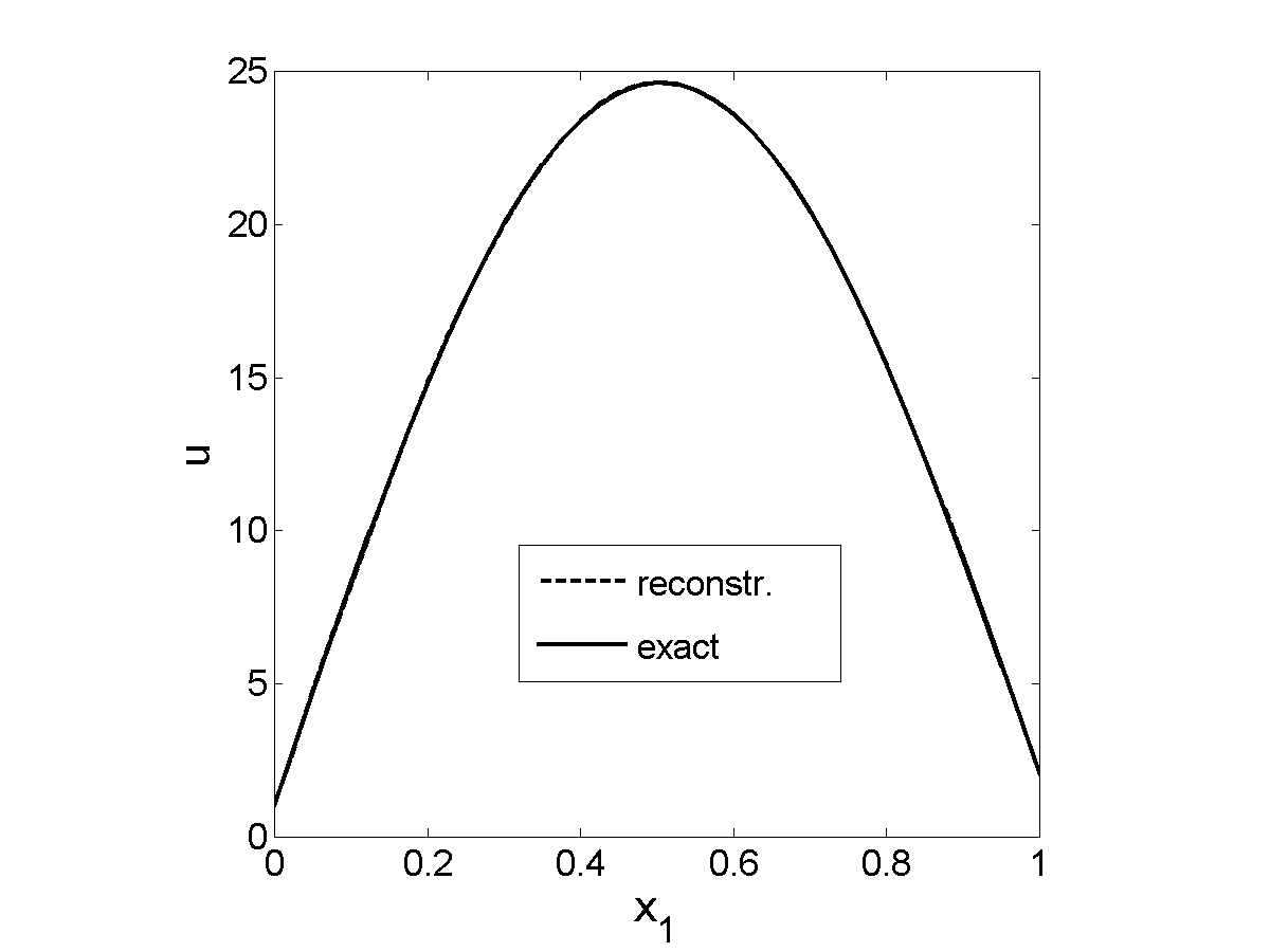
(a) noisy data of level $r=0.5$	(b) mean by $t$ model
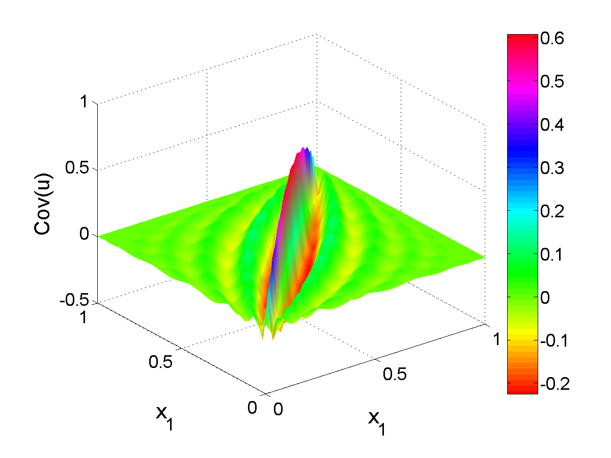
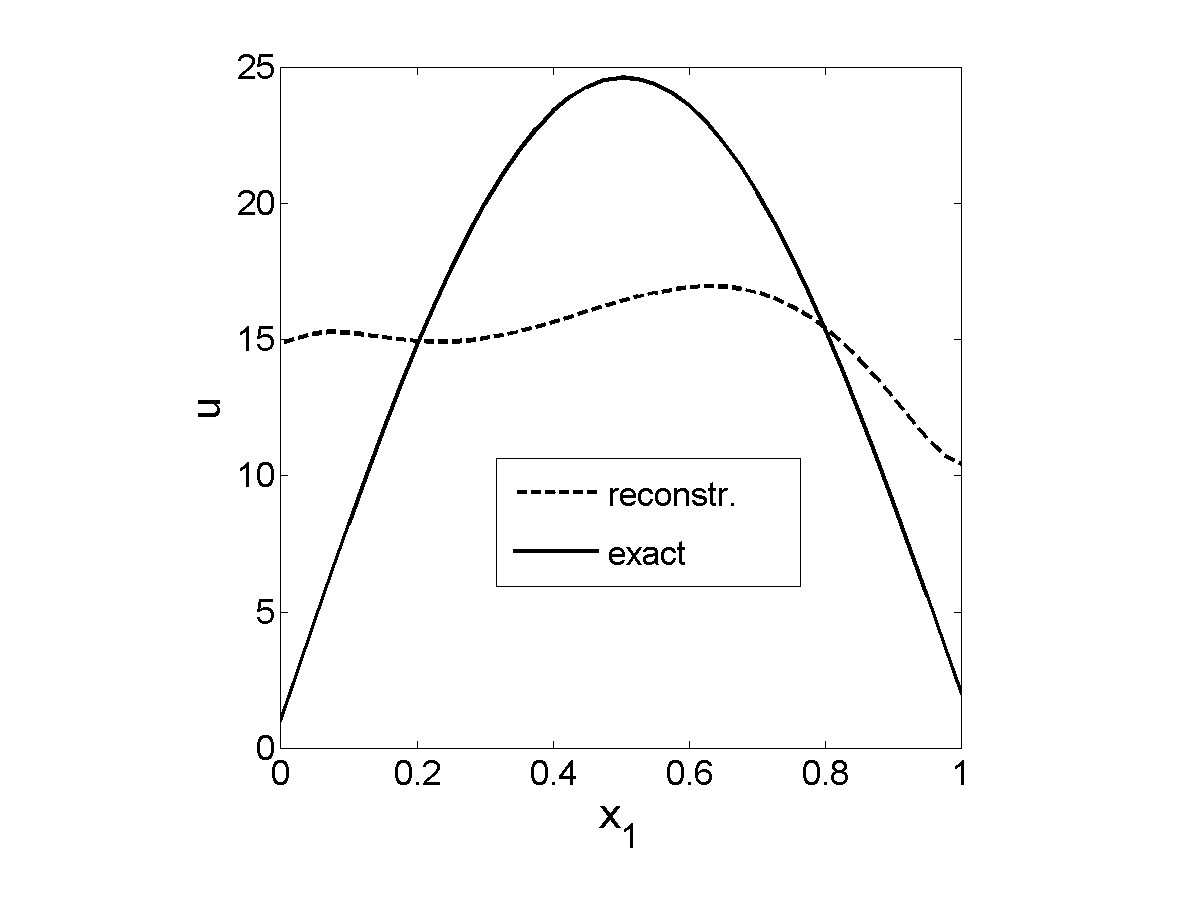
(c) covariance by $t$ model	(d) mean by Gaussian model
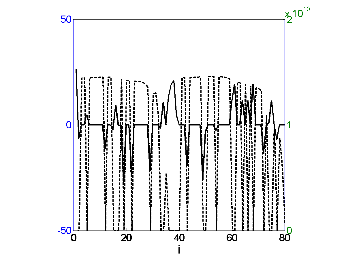
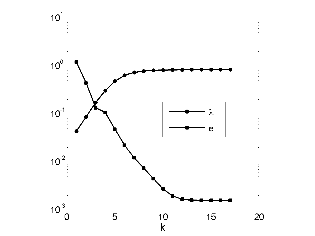
(e) weight $\mathbf{w}$ v.s. noise $\boldsymbol{\zeta}$	(f) Convergence of Alg. 1

Figure 2: Numerical results for Example 1 with $r=0.5$ noise. In (e), the solid and dashed lines refer to the noise $\boldsymbol{\zeta}$ and the weight $\mathbf{w}$, respectively.

4.2 Flux reconstruction

This example is taken from [39, Sect. 5.1]. Here, we consider 1d transient heat transfer. Let $\Omega$ be the interval $(0,1)$, and the time interval be $[0,1]$. The 1d transient heat conduction is described by

$$\frac{\partial y}{\partial t}=\Delta y,$$

with a zero initial condition and the following boundary conditions

$$\frac{\partial y}{\partial n}=g(t)\quad\mbox{on}\quad\Sigma_{c}\quad\quad\mbox{and}\quad\quad\frac{\partial y}{\partial n}=u(t)\quad\mbox{on}\quad\Sigma_{i},$$

where the boundaries $\Sigma_{c}=\{x=0\}\times[0,T]$ and $\Sigma_{i}=\{x=1\}\times[0,T]$. The operator $K$ maps the flux $u$ (with $g=0$) to $y$ restricted to $\Sigma_{c}$. The inverse problem is to recover the flux $u$ from noisy data $y$. For the inversion, we take $g(t)=0$ and a hat shaped flux $u$, see Fig. 3(b) for its profile. The spatial and temporal intervals are discretized into $101$ and $201$ uniform grids, respectively. The operator $K$ is discretized with piecewise linear finite elements in space and backward finite-difference in time. The number of measurements $\mathbf{y}$ is $50$, and the unknown $\mathbf{u}$ is on a coarse mesh and of size $51$.

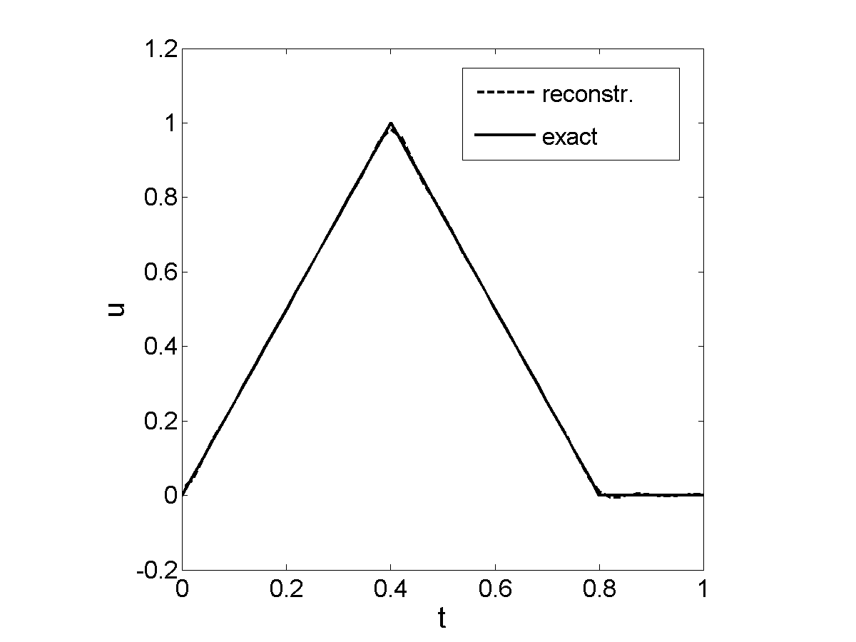
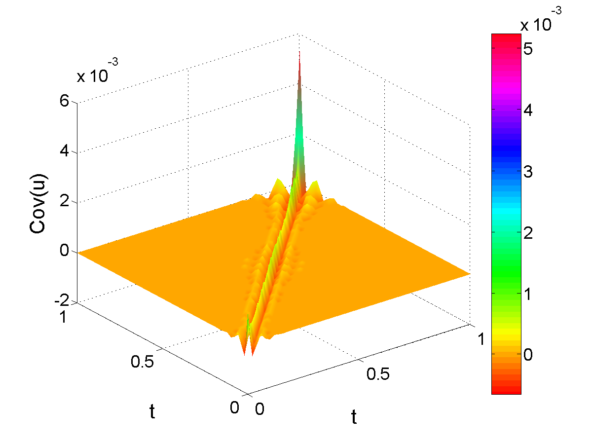
(a) mean by $t$ model	(b) covariance by $t$ model
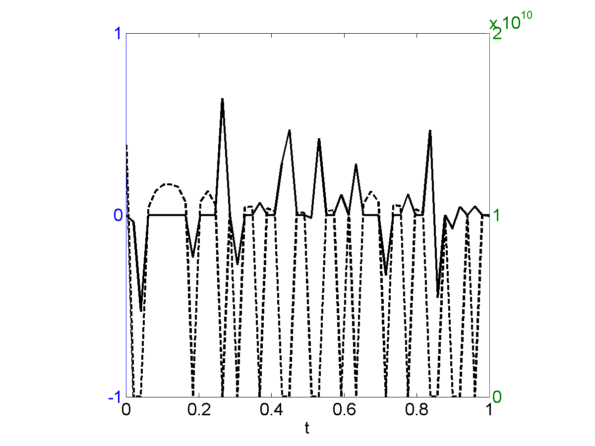
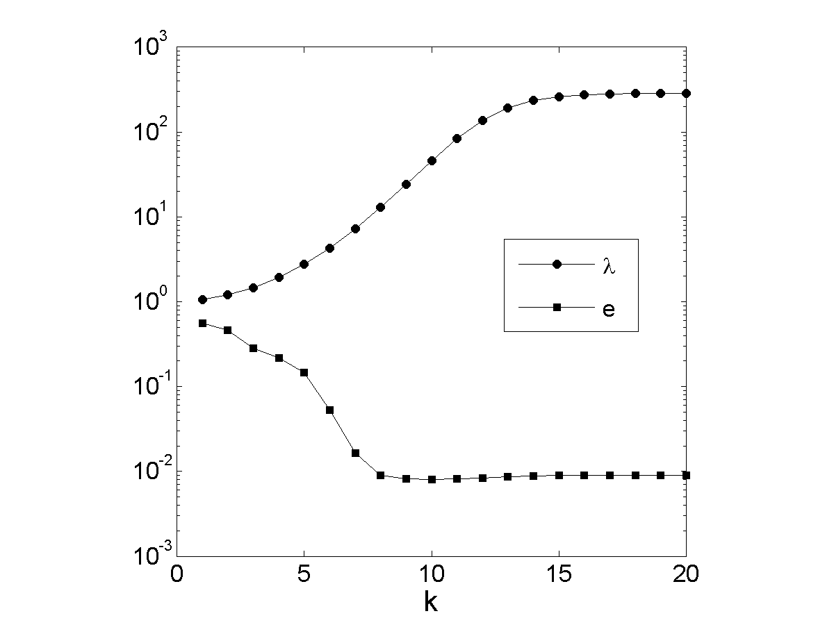
(c) weight $\mathbf{w}$ v.s. noise $\boldsymbol{\zeta}$	(d) convergence of Alg. 1

Figure 3: Numerical results for Example 2 with $r=0.5$ noise. In (c), the solid and dashed lines refer to the noise $\boldsymbol{\zeta}$ and the weight $\mathbf{w}$, respectively.

Table 2: Numerical results for Example 2 with various noise levels.

$r$	$0.1$	$0.2$	$0.3$	$0.4$	$0.5$	$0.6$	$0.7$	$0.8$
$\lambda$	3.29e2	3.20e2	3.04e2	2.97e2	2.86e2	2.71e2	2.55e2	2.44e2
$e$	5.51e-3	6.73e-3	8.17e-3	8.28e-3	9.06e-3	9.41e-3	1.79e-2	1.79e-2

The numerical results for Example 2 are shown in Table 2. The $\lambda$ value is independent of the corruption percentage $r$, and the accuracy $e$ only deteriorates very mildly with the increase of the corruption percentage $r$ from $0.1$ to $0.8$. The solution for a typical realization of noisy data of level $r=0.5$ is shown in Fig. 3(a), where $t$ is the temporal coordinate. It agrees excellently with the true solution, except small errors around the corner. The variance at the end points, especially around $t=1$, is much more pronounced than that in the interior, see Fig. 3(b). This might be related to the causality nature of heat problems. The weight $\mathbf{w}$ detects noise sites accurately and meanwhile eliminates them from the inversion by putting very small weight, and the convergence of the algorithm is steady and fast, c.f. Figs. 3(c) and (d), respectively.

4.3 Stationary Robin inverse problem

This example is adapted from [23, Sect. 5.2.4] [20], to illustrate the approach for nonlinear problems. Let $\Omega$ be the unit square $(0,1)^{2}$ with its boundary $\Gamma$ divided into two disjoint parts, i.e., $\Gamma_{i}=[0,1]\times\{1\}$ and $\Gamma_{c}=\Gamma\backslash\Gamma_{i}$. The steady-state heat conduction is described by

$$-\Delta y=0\quad\mbox{in }\Omega.$$

It is equipped with the following boundary conditions

$$\frac{\partial y}{\partial n}=g(x)\quad\mbox{on}\quad\Gamma_{c}\quad\quad\mbox{and}\quad\quad\frac{\partial y}{\partial n}+uy=0\quad\mbox{on}\quad\Gamma_{i},$$

where $u$ is the heat transfer coefficient. The operator $K$ maps the coefficient $u$ to $y$ restricted to $\Gamma_{c}$. The inverse problem is to reconstruct the unknown $u$ from noisy data $y$. It arises in corrosion detection [19, 24] and analysis of quenching process [33]. For the inversion, the flux $g$ is set to $1$, and the true coefficient $u$ is given by $1+\sin(\pi x_{1})$. The operator $K$ is discretized using piecewise linear finite element with $3200$ triangular elements. The number of measurements $\mathbf{y}$ is $120$, and the unknown $\mathbf{u}$ is of dimension $41$.

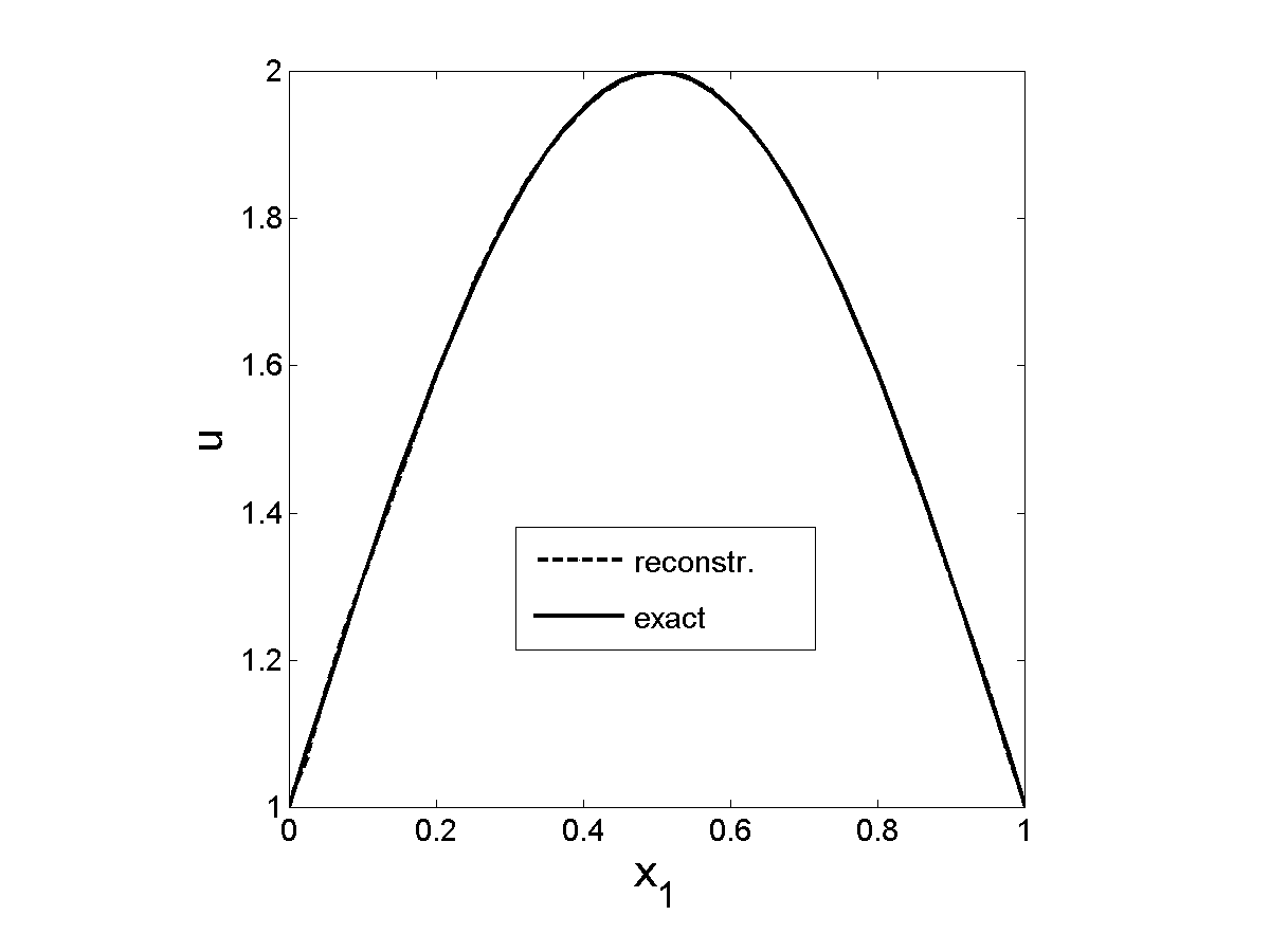
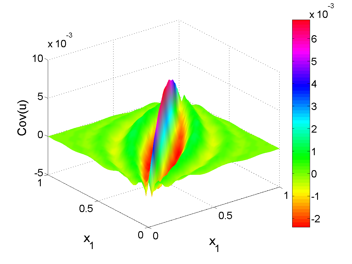
(a) mean by $t$ model	(b) covariance by $t$ model
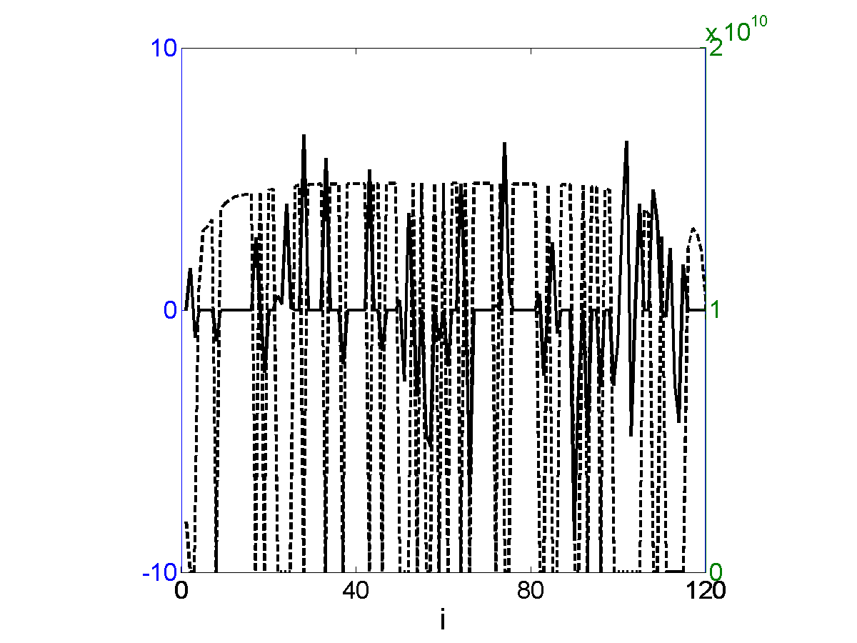
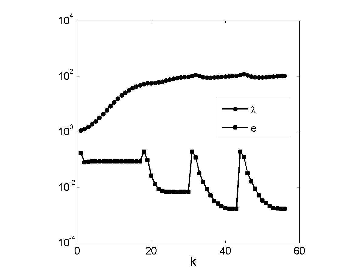
(c) weight $\mathbf{w}$ v.s. noise $\boldsymbol{\zeta}$	(d) convergence of Alg. 2

Figure 4: Numerical results for Example 3 with $r=0.5$ noise. In (c), the solid and dashed lines refer to the noise $\boldsymbol{\zeta}$ and the weight $\mathbf{w}$, respectively.

Table 3: Numerical results for Example 3 with various noise levels.

$r$	$0.1$	$0.2$	$0.3$	$0.4$	$0.5$	$0.6$	$0.7$	$0.8$	$0.9$
$\lambda$	1.07e2	1.04e2	1.03e2	1.03e2	1.03e2	1.03e2	1.02e2	1.01e2	9.78e1
$e$	1.30e-3	1.72e-3	1.71e-3	1.71e-3	1.70e-3	1.70e-3	1.69e-3	1.76e-3	2.27e-3

The numerical results for Example 3 are shown in Table 3. The observations for the linear models remain valid. The solution for an exemplary noise realization of level $r=0.5$ is shown in Fig. 4(a), which agrees well with the exact one. The convergence of Algorithm 2 is achieved within four (outer) iterations, see Fig. 4(d). The convergence behavior of the algorithm in the inner loop is similar to that of linear cases. The plateaus indicate that the tolerance $tol=1.0\times 10^{-5}$ is a bit too conservative, and the first two iterations may be solved less accurately without sacrificing the accuracy of the final solution.

4.4 Transient Robin inverse problem

This last example is adapted from [36]. Here we consider again 1d transient heat transfer. Let $\Omega$ be the spatial interval $(0,1)$, and the time interval be $[0,1]$. The 1d transient heat conduction is described by

$$\frac{\partial y}{\partial t}=\Delta y,$$

with a zero initial condition and the following boundary conditions

$$\frac{\partial y}{\partial n}=g(t)\quad\mbox{on}\quad\Sigma_{c}\quad\quad\mbox{and}\quad\quad\frac{\partial y}{\partial n}+uy=0\quad\mbox{ on }\Sigma_{i},$$

where $u(t)$ is a time-dependent heat transfer coefficient, and the boundaries $\Sigma_{c}=\{x=0\}\times[0,T]$ and $\Sigma_{i}=\{x=1\}\times[0,T]$. The operator $K$ maps the coefficient $u$ to $y$ restricted to $\Sigma_{c}$. The inverse problem is to estimate the coefficient $u$ from noisy data $y$ [36, 21]. For the inversion, the flux $g$ is set to $1$, and the true coefficient $u=1+\frac{1}{2}\chi_{[\frac{3}{10},\frac{7}{10}]}$ is discontinuous, where $\chi$ denotes the characteristic function. The spatial and temporal intervals are both discretized into $100$ uniform intervals. The operator $K$ is discretized with piecewise linear finite elements in space and backward finite-difference in time. The number of measurements $\mathbf{y}$ is $101$, and the the unknown $\mathbf{u}$ is of dimension $101$.

Table 4: Numerical results for Example 4 with various levels.

$r$	$0.1$	$0.2$	$0.3$	$0.4$	$0.5$	$0.6$	$0.7$	$0.8$	$0.9$
$\lambda$	2.25e2	2.23e2	2.23e2	2.26e2	2.27e2	2.27e2	2.32e2	2.34e2	2.29e2
$e$	3.94e-2	3.97e-2	3.98e-2	4.05e-2	4.11e-2	4.14e-2	4.25e-2	4.31e-2	4.32e-2

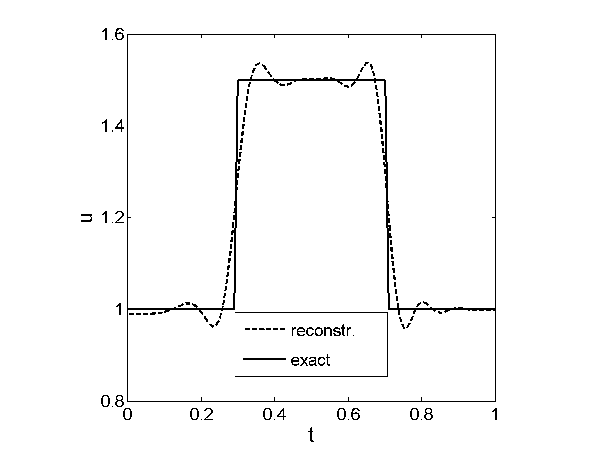
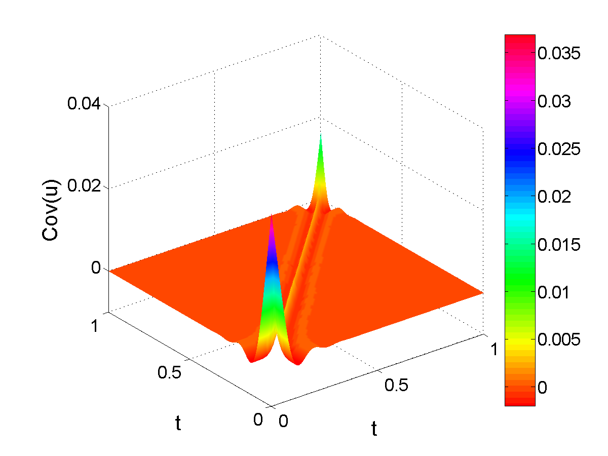
(a) mean by $t$ model	(b) covariance by $t$ model
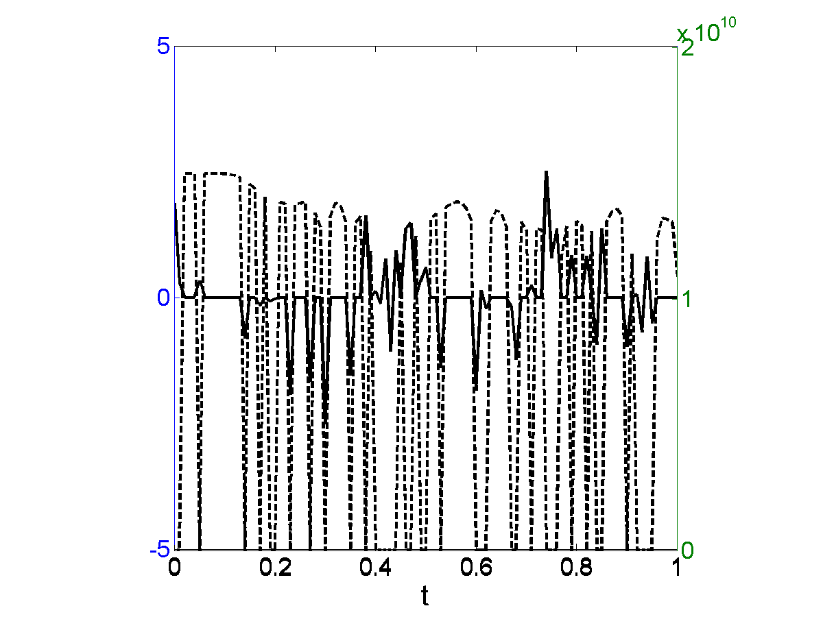
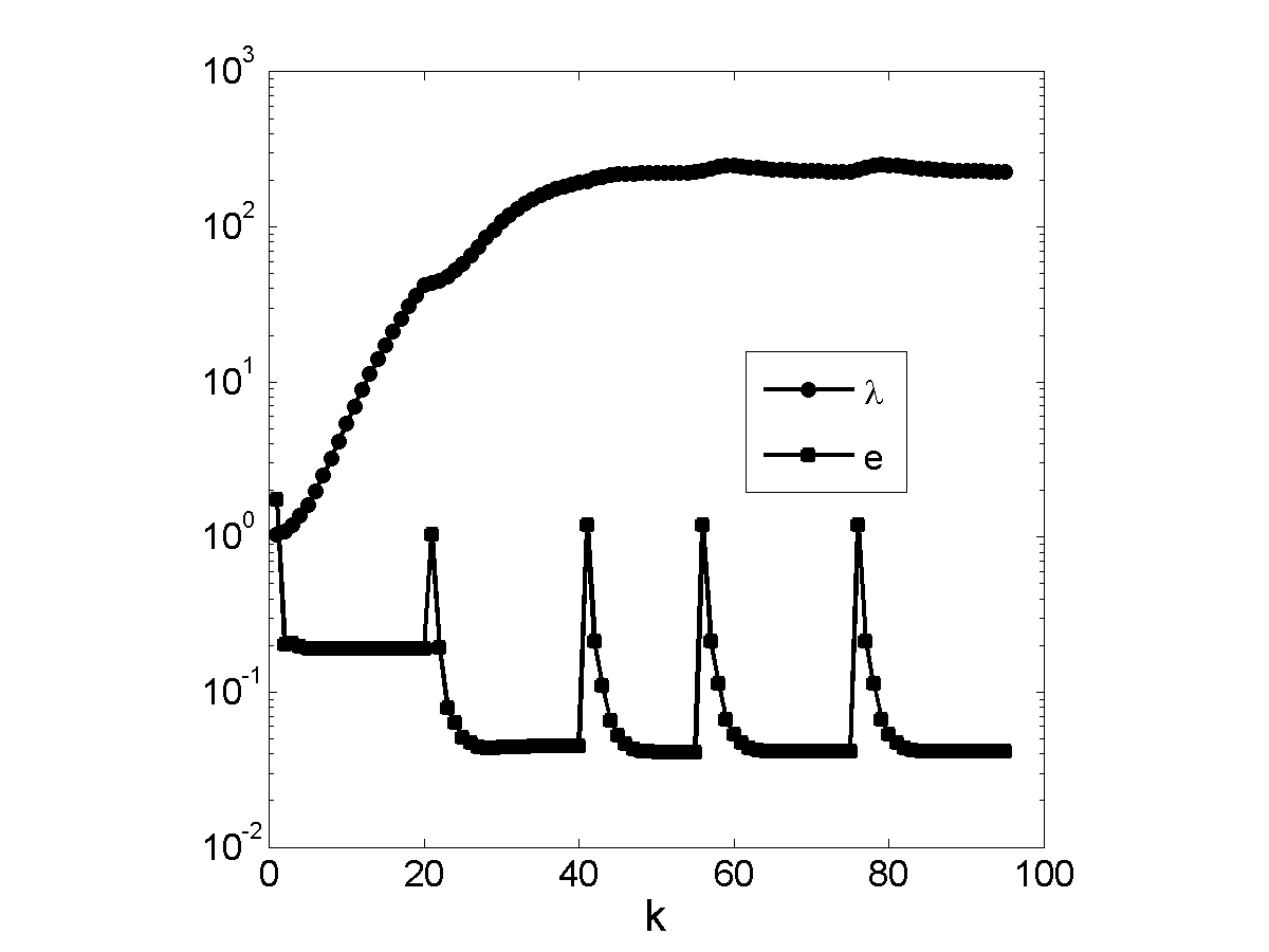
(c) weight $\mathbf{w}$ v.s. noise $\boldsymbol{\zeta}$	(d) convergence of Alg. 2

Figure 5: Numerical results for Example 4 with $r=0.5$ noise. In (c), the solid and dashed lines refer to the noise $\boldsymbol{\zeta}$ and the weight $\mathbf{w}$, respectively.

The numerical results for Example 4 with data of various noise levels are shown in Table 4. The accuracy $e$ only deteriorates very mildly as the corruption percentage $r$ increases from $0.1$ to $0.9$. The result for a typical realization of noisy data with $r=0.5$ is shown in Fig. 5. The solution is not as accurate as before, since it oscillates slightly around the discontinuities of the true solution. This is a consequence of the smoothness prior adopted here, which in principle is unsuited to reconstructing discontinuous profiles. Nonetheless, the solution is reasonable as the overall profile of the true solution is largely retrieved, and the magnitude is accurate. The convergence of Algorithm 2 remains very stable for the discontinuous solution. However, there are several large plateaus, which might be pruned out by increasing the tolerance $tol$ so as to effect the desired computational speedup.

5 Concluding remarks

In this paper we have developed a robust Bayesian approach to inverse problems subject to impulsive noises. It explicitly adopts a heavy-tailed $t$ model to cope with data outliers, and it admits a scale mixture representation, which enables deriving efficient variational algorithms. The approach has been illustrated on several benchmark linear and nonlinear inverse problems arising in heat transfer. The numerical results are accurate and stable even in the presence of a fairly large amount of data outliers, and it is much more robust compared with the conventional Gaussian model.

There are several avenues deserving further research. We have restricted our attention to the simplest Markov random field. A natural research problem would be the extension to general random fields, especially sparsity-promoting prior. Second, it is useful to develop alternative techniques, e.g., based on the Laplace model, and to compare their merits. The method can only achieve reasonable computational efficiency for medium-scale problems due to the variance component. It is of interest to develop scalable algorithms by imposing further restrictions on the approximation. Lastly, rigorous justification of the excellent performance of the model as well as the algorithm, e.g., consistency and convergence rate, is of immense theoretical importance, and is to be established.

References

- [1] A. Achim, A. Bezerianos, and P. Tsakalides. Novel Bayesian multiscale method for speckle removal in medical ultrasound images. IEEE Trans. Med. Imag., 20(8):772–783, 2001.
- [2] S. Alliney and S. Ruzinsky. An algorithm for the minimization of mixed l1 and l2 norms with application to Bayesian estimation. IEEE Trans. Signal Process., 42(3):618–627, 1994.
- [3] H. Attias. A variational Bayesian framework for graphical models. In Advances in Neural Information Processing Systems, volume 12, pages 209–215, 2000.
- [4] M. J. Beal. Variational Algorithms for Approximate Bayesian Inference. PhD thesis, Gatsby Computational Neuroscience Unit, University College London, 2003.
- [5] J. V. Beck, B. Blackwell, and C. R. St. Clair. Inverse Heat Conduction: Ill-Posed Problems. Wiley, New York, 1985.
- [6] R. H. Chan, C.-H. Ho, and M. Nikolova. Salt-and-pepper noise removal by median-type noise detectors and detail-preserving regularization. IEEE Trans. Imag. Process., 14(10):1479–1485, 2005.
- [7] M. A. Chappell, A. R. Groves, B. Whitcher, and M. W. Woolrich. Variational Bayesian inference for a nonlinear forward model. IEEE Trans. Signal Process., 57(1):223–236, 2009.
- [8] S. C. Choi and R. Wette. Maximum likelihood estimation of the parameters of the Gamma distribution and their bias. Technometrics, 11(4):683–690, 1969.
- [9] C. Clason, B. Jin, and K. Kunisch. A duality-based splitting method for - image restoration with automatic regularization parameter choice. SIAM J. Sci. Comput., 32(3):1484–1505, 2010.
- [10] C. Clason, B. Jin, and K. Kunisch. A semismooth Newton method for data fitting with automatic choice of regularization parameters and noise calibration. SIAM J. Imaging Sci., 3(2):199–231, 2010.
- [11] P. Colli-Franzone, L. Guerri, S. Tentoni, C. Viganotti, S. Baruffi, S. Spaggiari, and B. Taccardi. A mathematical procedure for solving the inverse potential problem of electrocardiography: analysis of the time-space accuracy from in vitro experimental data. Math. Biosci., 77(1–2):353–396, 1985.
- [12] A. P. Dempster, N. M. Laird, and D. B. Rubin. Maximum likelihood from incomplete data via the EM algorithm. J. Royal Stat. Soc., Ser. B, 39(1):1–38, 1977.
- [13] A. F. Emery. Parameter estimation in the presence of uncertain parameters and with correlated data errors. Int. J. Thermal Sci., 41(6):481–491, 2002.
- [14] A. F. Emery. Estimating deterministic parameters by Bayesian inference with emphasis on estimating the uncertainty of the parameters. Inv. Probl. Sci. Eng., 17(2):263–274, 2009.
- [15] J. Gao. Robust principal component analysis and its Bayesian variational inference. Neur. Comput., 20(2):555–572, 2008.
- [16] A. Gelman, J. B. Carlin, H. S. Stern, and D. B. Rubin. Bayesian Data Analysis. Chapman & Hall/CRC, Boca Raton, FL, 2nd edition, 2004.
- [17] J. Geweke. Bayesian treatment of the independent student- t linear model. J. Appl. Econometrics, 8(S):S19–40, 1993.
- [18] T. Hebert and R. Leahy. A generalized EM algorithm for 3-d Bayesian reconstruction from Poisson data using Gibbs priors. IEEE Trans. Med. Imag., 8(2):194–202, 1989.
- [19] G. Inglese. An inverse problem in corrosion detection. Inverse Problems, 13(4):977–994, 1997.
- [20] B. Jin. Fast Bayesian approach for parameter estimation. Int. J. Numer. Methods Engrg., 76(2):230–252, 2008.
- [21] B. Jin and X. Lu. Numerical identification of a robin coefficient in parabolic problems. Math. Comput., page in press., 2011.
- [22] B. Jin and J. Zou. Augmented Tikhonov regularization. Inverse Problems, 25(2):025001, 25, 2009.
- [23] B. Jin and J. Zou. Hierarchical Bayesian inference for ill-posed problems via variational method. J. Comput. Phys., 229(19):7317–7343, 2010.
- [24] B. Jin and J. Zou. Numerical estimation of the Robin coefficient in a stationary diffusion equation. IMA J. Numer. Anal., 30(3):677–701, 2010.
- [25] M. I. Jordan, Z. Ghahramani, T. S. Jaakkola, and L. K. Saul. An introduction to variational methods for graphical models. Mach. Learn., 37:183–233, 1999.
- [26] J. Kaipio and E. Somersalo. Statistical and Computational Inverse Problems. Springer-Verlag, New York, 2005.
- [27] J. P. Kaipio, V. Kolehmainen, E. Somersalo, and M. Vauhkonen. Statistical inversion and Monte Carlo sampling methods in electrical impedance tomography. Inverse Problems, 16(5):1487–1522, 2000.
- [28] P. S. Koutsourelakis. A multi-resolution, non-parametric, Bayesian framework for identification of spatially-varying model parameters. J. Comput. Phys., 228(17):6184–6211, 2009.
- [29] K. L. Lange, R. J. A. Little, and J. M. G. Taylor. Robust statistical modeling using the distribution. J. Amer. Statist. Assoc., 84(408):881–896, 1989.
- [30] X. Ma and N. Zabaras. An efficient Bayesian inference approach to inverse problems based on an adaptive sparse grid collocation method. Inverse Problems, 25(3):035013, 27, 2009.
- [31] Y. Marzouk and D. Xiu. A stochastic collocation approach to Bayesian inference in inverse problems. Comm. Comput. Phys., 6(4):826–847, 2009.
- [32] Y. M. Marzouk, H. N. Najm, and L. A. Rahn. Stochastic spectral methods for efficient bayesian solution of inverse problems. J. Comput. Phys., 224(2):560–586, 2007.
- [33] A. M. Osman and J. V. Beck. Nonlinear inverse problem for the estimation of time-and-space dependent heat transfer coefficients. J. Thermophys., 3:146–152, 1988.
- [34] M. Sambridge and K. Mosegaard. Monte Carlo methods in geophysical inverse problems. Rev. Geophys., 40(3):3–29, 2002.
- [35] M. Sato, T. Yoshioka, S. Kajihara, K. Toyama, N. Goda, K. Doya, and M. Kawato. Hierarchical Bayesian estimation for MEG inverse problem. NeuroImage, 23(3):806–826, 2004.
- [36] J. Su and G. F. Hewitt. Inverse heat conduction problem of estimating time-varying heat transfer coefficient. Numer. Heat Transfer, Part A, 45(8):777–789, 2004.
- [37] A. Tarantola. Inverse Problem Theory and Methods for Model Parameter Estimation. SIAM, Philadelphia, PA, 2005.
- [38] M. E. Tipping and N. D. Lawrence. Variational inference for student-t models: robust bayesian interpolation and generalised component analysis. Neurocomput., 69(1–3):123–141, 2005.
- [39] J. Wang and N. Zabaras. A Bayesian inference approach to the inverse heat conduction problem. Int. J. Heat Mass Transfer, 47(17-18):3927–3941, 2004.
- [40] J. Wang and N. Zabaras. Hierarchical Bayesian models for inverse problems in heat conduction. Inverse Problems, 21(1):183–206, 2005.