High-order regularized regression in Electrical Impedance Tomography

Abstract

We present a novel approach for the inverse problem in electrical impedance tomography based on regularized quadratic regression. Our contribution introduces a new formulation for the forward model in the form of a nonlinear integral transform, that maps changes in the electrical properties of a domain to their respective variations in boundary data. Using perturbation theory the transform is approximated to yield a high-order misfit function which is then used to derive a regularized inverse problem. In particular, we consider the nonlinear problem to second-order accuracy, hence our approximation method improves upon the local linearization of the forward mapping. The inverse problem is approached using Newton’s iterative algorithm and results from simulated experiments are presented. With a moderate increase in computational complexity, the method yields superior results compared to those of regularized linear regression and can be implemented to address the nonlinear inverse problem.

keywords: Impedance tomography transform, quadratic regression, Newton’s method

1 Introduction

In Electrical Impedance Tomography (EIT) voltage measurements captured at the boundary of a conductive domain are used to estimate the spatial distribution of its electrical properties. The technique has numerous applications in exploration geophysics [45], environmental monitoring and hydrogeophysics [5], [24], biomedical imaging [17], industrial process monitoring [39], archaeological site assessment [34] and non-destructive testing of materials [38]. Owing to its many practical uses and intriguing mathematics, EIT has seen numerous theoretical and computational developments, e.g. the the chapter expositions in [1], [25] and [22]. Among its fundamental challenges remain the nonlinearity and ill-posedness of the inverse problem, which inevitably compromise the spatial resolution of the reconstructed images. From the mathematical prospective, this inverse boundary value problem, formalized by the seminal publication of Caldéron [8], presents a number of implications on the existence, uniqueness and numerical stability of the solution [6], [1]. Although the issues of existence and uniqueness can be eradicated under some mild assumptions, see for example [41] for isotropic conductivity fields, the instability causes the problem to be extremely sensitive to inaccuracies and small errors in the data. To alleviate the ill-posedness one usually resorts in implementing some type of regularization strategy that stabilizes the solution [18]. Based on prior information about the unknown electrical parameters and/or the noise statistics in the measurements, regularization schemes are applied in order to stabilize the reconstructions. In the typical variational framework for example, regularization methods are often expressed as additive penalty terms augmenting the associated data misfit function, essentially biasing the solution away from features that are inconsistent with the available a priori information. In this sense, [20] examines the case of Tikhonov regularization in the context of nonlinear system identification emphasizing the bias-variance trade-off on the solution.

The nonlinearity inevitably increases the complexity of the problem, as the data misfit function has several local minima, and hence one is faced with the challenge of locating the solution that corresponds to the global minimum. Aside a few notable exceptions, like the d-bar method [26] and the factorization method [15], algorithms that treat the nonlinearity are essentially Newton-type iterative solvers, such as the often used Gauss–Newton (GN) method, that implement local linearization and regularization, essentially exploiting the Fréchet differentiability of the analytic forward operator, to yield at each iteration a quadratic error function with respect to the unknown parameters [9], [32]. Starting from a feasible guess and, in some cases, an estimate of the noise level in the data, one applies a number of linearization–regularization cycles until a convergence is reached in the sense of the discrepancy principle. Analysis on the convergence rates of the GN algorithm and quasi-Newton variants for high-dimensional problems can be found in [3], [18] and [23], and [14]. These results state that convergence is not guaranteed unless a stable Newton direction, descent in the usual case of minimization, is computed at each linearization point. In turn, this relies on the optimal tuning of regularization at each iteration, indeed a delicate and challenging task as the degree of ill-posedness may vary significantly [27]. To rectify this problem and aid convergence line search algorithms can be used, that scale optimally the solution increment in the descent Newton direction [4], as indeed trust-region methods [10] although more computationally complex. An additional important complication may arise when the typically-neglected linearization error is significantly large, invariably when the linearization point is ‘not close enough’ to the true solution [36]. This implies that a component of the linearized data should not be considered in the fitting process, since local linearization approximation is accurate in a rather narrow trust region, and hence to cope with the lack of this information at each iteration one seeks to recover a ‘small’ perturbation of the parameters. With this as background, the work in this paper focusses on the following contributions: (i) A nonlinear integral transform as a forward model that maps arbitrarily large, bounded changes in electrical properties to changes in boundary observations. Effectively, this replaces the linear approximation involving the Jacobian of the forward mapping [29]. The transform has a closed form and admits a numerical approximation using the finite element method. (ii) Exploiting the new model, a high-order misfit function is formulated for the inverse problem in the context of regularized regression. Numerical experiments on the resulting inverse problem have yield solutions with small image errors and adequate spatial resolution.

Higher-order derivatives are thus seldom used in inversion schemes since the increase in convergence rates may not compensate adequately for the computational effort required in computing the derivatives, in particular when high-dimensional discrete models with tensor parameters are concerned. Moreover, if the data misfit residual is small then the error contribution of the higher-order terms becomes negligibly small. The majority of inversion algorithms, as indeed the general theory, for nonlinear inverse problems utilize merely a first-order approximation of the underlying model [18]. A notable exception is the second-order method for nonlinear, highly ill-posed parameter identification problems in some classical partial differential equations, such as Helmholtz, diffusion and Sturm-Liouville [16]. In [16], the authors propose iterative predictor-corrector schemes encompassing Tikhonov regularization that approximate the second-order solution without solving a quadratic equation. Using this computationally efficient framework, they report on advantages in the final reconstructions and significant improvements in the number of iterations required for convergence.

As we develop our methodology we address mainly the EIT problem with complex isotropic admittivity and the complete electrode boundary conditions [40]. However, our derivations are not constrained by isotropic or complex property assumptions and thus can be easily shown to hold true for the similar problems of Electrical Resistance and Capacitance Tomography (ERT/ECT) with purely real coefficients in scalar or tensor field material properties [1], [33]. Moreover, we show that the form of the new forward model remains unchanged with the governing elliptic differential equation is addressed in the context of more generalized boundary conditions that resemble more simplistic electrode models conventionally encountered in the geophysical setting [5],[2].

1.1 Notation and paper organization

Consider a simply connected domain $B\subset\mathbb{R}^{d}$, $d=2,3$ with Lipschitz smooth boundary $\partial B$ and a space depended isotropic admittivity function $\gamma(\mathbf{x},\omega):B\rightarrow\mathbb{C}$. At an angular frequency $\omega\geq 0$, the admittivity can be expressed as

$$\gamma(\mathbf{x},\omega)=\sigma(\mathbf{x})+i\omega\epsilon(\mathbf{x}),$$

where $\infty>C_{1}>\sigma>c_{1}>0$ and $\infty>C_{2}>\epsilon\geq 0$ denote the domain’s electrical conductivity and permittivity respectively for some positive bounding constants $C_{1},\,C_{2},\,c$. If there are no charges or sources in the interior of $B$ and the angular frequency of the applied currents is small enough, then Maxwell’s equations describing the electromagnetic fields in the interior of the domain reduce to the elliptic equation

$$\nabla\cdot[\gamma(\mathbf{x},\omega)\nabla u(\mathbf{x},\omega)]=0,\quad\mathbf{x}\in B,$$ (1)

where $u$ denotes the scalar electric potential function. Measuring the potential at the accessible parts of the boundary of the domain through a finite number of sensors yields a set of observations $\zeta$ that are likely to suffer from some type of noise and measurement imprecision $\eta$. We will assume EIT systems equipped with $L$ electrodes exciting the domain with a sequence of currents $I\doteq(I^{1},\ldots,I^{q})$, with $I^{i}\doteq(I_{1},\ldots,I_{L})$ all fixed at frequency $\omega$. In such a case $\zeta$ is typically a linear combination of the electrode potentials $U(I^{i})\doteq(U_{1},\ldots,U_{L})$, for $i=1,\ldots,q$ at the various current patterns. For an applied current pattern $I$ we associate an electric potential field $u$ in $\overline{B}$, and an array of electrode potentials $U$ at $\partial B$. When required by the context we shall denote their dependence on admittivity and applied current as $u(\gamma)$ and $u(I)$, or both as $u(\gamma,I)$; and respectively $U(\gamma)$, $U(I)$ and $U(\gamma,I)$. The first and second partial derivatives of $u$ with respect to $\gamma$ will be denoted by $\partial_{\gamma}u$ and $\partial_{\gamma\gamma}u$, a notation adopted for both continuous and discrete spatial functions, while for matrices and vectors the differentiation is to be considered element-wise. The position in $\overline{B}$ is specified by the vector $\mathbf{x}\in\mathbb{R}^{d}$, while the outward unit normal vector at the boundary is denoted $\mathbf{n}$. Matrices and vector fields are expressed in bold capital letters while vectors and scalar fields in small case regular. For a matrix $\bf A$, $a_{j}$ will denote the $j$th row, $\mathbf{A}_{i,j}$ its $(i,j)$th element and $\bf A^{\prime}$ its transpose. For a vector $v$, $v_{i}$ is the $i$th element and $\bar{v}$ is the complex conjugate. The spaces of real and complex numbers are given by $\mathbb{R}$ and $\mathbb{C}$, while we use $\Re\{c\}$ to express the real component of the complex argument $c$.

The paper is organized as follows: We begin with a brief review of the the EIT model equations and associated preliminary concepts and then proceed to formulate the inverse problem commenting on existing algorithms the address the problem through local linearization. The next section is devoted to the derivation of the nonlinear integral transform under the complete electrode model and its generalization to the Poisson’s equation with mixed boundary conditions. Further on we consider the high-order regularized regression problem and approximate the nonlinear system as a quadratic operator equation. Using the finite element we obtain a numerical approximation and subsequently implement Newton’s algorithm to solve the problem. Finally, we present numerical results from simulated studies that demonstrate the advantages of the proposed methodology and we end the paper with the conclusions section.

2 EIT model equations and preliminaries

The complete electrode model in electrical impedance tomography is derived from Maxwell’s time-harmonic equations at the quasi-static limit and describes the electric potential field in the closure of a conductive domain $B$ with known electrical properties $\gamma$ and impressed boundary excitation conditions. The model has been extensively reviewed and analyzed in several publications, including [40] where the authors prove the existence and uniqueness of the solution, under some continuity assumptions on the interior admittivity. With reference to figure 1, assuming no charges or current sources in the interior of $B$, when a current is applied at the boundary, the electric potential $u$ satisfies the elliptic partial differential equation (1). The applied current, inducing this field, is expressed by the Neumann boundary conditions

$$\int_{e_{\ell}}\mathrm{d}s\; \gamma(\mathbf{x},\omega)\nabla u(\mathbf{x})\cdot\mathbf{n}= I_{\ell},\quad\mathbf{x}\in\Gamma_{e_{\ell}},\;\ell=1,\ldots,L,$$ (2)

$$\gamma(\mathbf{x},\omega)\nabla u(\mathbf{x})\cdot\mathbf{n}= 0,\quad\;\mathbf{x}\in\partial B\setminus\Gamma_{e},$$ (3)

where $\Gamma_{e}=\bigcup_{\ell=1}^{L}\Gamma_{e_{\ell}}$. An accurate model of the electrodes is critical when comparing experimental measurements to synthetic model predictions. In effect, the voltage measurement recorded at the $\ell$th electrode with contact impedance $z_{\ell}$ is given by the Robin condition

$$U_{\ell}=u(\mathbf{x})+z_{\ell}\gamma(\mathbf{x},\omega)\nabla u(\mathbf{x})\cdot\mathbf{n},\quad\mathbf{x}\in\Gamma_{e_{\ell}},\;\ell=1,\ldots,L,$$ (4)

assuming that the characteristic function of the contact impedance is uniform on each electrode and $\Re\{z_{\ell}\}>0$. The model admits a unique solution $(u,U)$ upon enforcing the charge conservation principle on the applied currents and a choice of ground is made. Maintaining the conventional notation of [40], [25], and [6] we these constraints imply

$$\sum_{\ell=1}^{L}I_{\ell}=0,\quad\text{and}\quad\int_{\partial B}\mathrm{d}s\,u=0,$$ (5)

where the applied currents should sum up to zero and the induced potential should have a vanishing mean on the boundary. For the so-called forward or direct problem (1)-(5) we adopt the following essential assumptions [25], [22].

Assumption 1

(a) The domain $B$ is simply connected with boundary $\partial B$ at least Lipschitz continuous.
(b) The electrical admittivity $\gamma\in L^{\infty}(\overline{B})$ with $\operatorname*{ess\,inf}(\gamma)>c_{1}>0$.
(c) The potential field $u\in H^{1}_{o}(B)=\{u\in H^{1}(B):\int_{\partial B}\mathrm{d}s\,u=0\}$
(d) The applied currents $I$ and measured voltages $\zeta$ belong in the Hilbert spaces of the $L$, and respectively $m$ dimensional complex vectors $\mathbb{C}^{L}$ and $\mathbb{C}^{m}$, where $m\geq L$.

Figure 1: The domain under consideration $B$ with $L$ round surface electrodes $\Gamma_{e_{\ell}}$ attached at the boundary $\Gamma_{e}$.

We will often refer to the solution $(u,U)\in H_{o}^{1}(B)\oplus\mathbb{C}^{L}$ as the direct solution, and to the problem (1)-(5) as the direct problem. Pertinent to this model is the adjoint forward problem [2]. Consider the direct solution under a pair drive current pattern $I^{d}$ with positive and negative polarity applied at electrodes $e_{p}$ and $e_{n}$ respectively. Moreover, let the $k$’th boundary measurement be of the form

$$\zeta_{k}=U_{e_{p^{\prime}}}-U_{e_{n^{\prime}}},\quad p^{\prime},n^{\prime}\in\{1,\ldots,L\},\quad k=1,\ldots,m$$

for a pair of electrodes $e_{p^{\prime}}$ and $e_{n^{\prime}}$. In the practical setting of EIT or ERT, see for example the applications discussed in [17], [13], [24] and [43], instead of measuring the electrode potentials, it is usual to measure the potential between adjacent electrodes. When captured systematically, this differential type of measurement yields $m\geq L$ linearly independent data. Based on this measurement definition, the adjoint field solution $(v,V)\in H_{o}^{1}(B)\oplus\mathbb{C}^{L}$ satisfies the equations

$$\nabla\cdot[\overline{\gamma}(\mathbf{x},\omega)\nabla v(\mathbf{x})] = 0\quad\mathbf{x}\in B,$$ (6)

$$\overline{\gamma}(\mathbf{x},\omega)\nabla v(\mathbf{x})\cdot\mathbf{n} = 0\quad\mathbf{x}\in\partial B\setminus\Gamma_{e},$$ (7)

$$\int_{e_{\ell}}\mathrm{d}s\,\overline{\gamma}(\mathbf{x},\omega)\nabla v(\mathbf{x})\cdot\mathbf{n} = I^{m}_{\ell}\quad\mathbf{x}\in\Gamma_{e_{\ell}},$$ (8)

$$v(\mathbf{x})+z_{\ell}\overline{\gamma}(\mathbf{x},\omega)\nabla v(\mathbf{x})\cdot\mathbf{n} = V_{\ell},\quad\mathbf{x}\in\Gamma_{e_{\ell}},\;\ell=1,\ldots,L$$ (9)

where $\overline{\gamma}(\mathbf{x},\omega)=\gamma(\mathbf{x},-\omega)$ is the conjugated admittivity, and $I^{m}\in\mathbb{C}^{L}$ is the adjoint current pattern whose $\ell$’th entry equals to $I^{m}_{\ell^{\prime}}=\overline{I^{d}_{\ell}}$, if $\ell=e_{p}$ or $\ell=e_{n}$ and zero otherwise. The uniqueness of the adjoint solution is subject to the constraints of the type in (5).

2.1 Green’s reciprocity

In what follows, we make reference to the reciprocity principle. Originally derived from Maxwell’s laws of electromagnetics, Maxwell’s reciprocity principle has an analogue for irrotational fields known as Green’s reciprocity. In the context of the impedance experiment it states, that if a current intensity $I$ is applied at the boundary of a closed domain between two electrodes, say $P_{1}\doteq(e_{p},e_{n})$, then the potential measured at the boundary through another pair of electrodes $P_{2}\doteq(e_{p^{\prime}},e_{n^{\prime}})$ will be equal to the potential measured at $P_{1}$ if the same current is applied to $P_{2}$. Impedance data acquisition instruments rely on this principle to avoid making redundant, i.e. linearly dependent, measurements. To see this consider a linear conductive medium $B$ whose admittivity $\gamma$ has a nonzero imaginary component at the operating non-resonant frequency $\omega$. Suppose we apply a time-harmonic electric current $I^{d}$ at the boundary of the domain through electrodes $P_{1}$,

$$I^{d}(\mathbf{x},t)=\mathbf{J}(\mathbf{x},\omega)\,e^{i\omega t},\qquad\mathbf{x}\in\partial B,$$

where $\mathbf{J}$ is the current density field. From Maxwell’s laws the electric and magnetic fields $\mathbf{E}$, and $\mathbf{H}$, within the domain satisfy

$$\nabla\times\mathbf{H}(\mathbf{x})=\gamma(\mathbf{x})\mathbf{E}(\mathbf{x}),\qquad\mathbf{x}\in\overline{B}.$$

As the domain is simply connected, using $\mathbf{E}(\mathbf{x})=-\nabla u(\mathbf{x})$ and $\nabla\times\mathbf{H}(\mathbf{x})=\mathbf{J}(\mathbf{x})$ reduces to Ohm’s law

$$\mathbf{J}(\mathbf{x})=-\gamma(\mathbf{x})\nabla u(\mathbf{x}).$$ (10)

Let the magnitude of the applied current be equal to $I_{o}$, such that $|I^{d}_{e_{p}}|=I_{o}$ and $I^{d}_{e_{n}}=-I^{d}_{e_{p}}$. Similarly, allow $I^{m}$ a different current pattern of unit magnitude applied through a different pair of boundary electrodes, say $P_{2}$, inducing a new electric potential field. We denote the two fields as $u(I^{d})$ and $u(I^{m})$ to emphasize their dependance on the excitation currents. Taking the normal component of the vector fields in (10) for $I^{d}$, multiplying with $u(I^{m})$ and integrating over the boundary yields

$$\int_{\partial B}\mathrm{d}s\;u(I^{m})\mathbf{J}(I^{d})\cdot\mathbf{n}=-\int_{\partial B}\mathrm{d}s\;\gamma\,u(I^{m})\nabla u(I^{d})\cdot\mathbf{n}.$$

At $\mathbf{x}\in\partial B$, let $j(\mathbf{x})=\mathbf{J}(\mathbf{x})\cdot\mathbf{n}$ be the normal component of the boundary current density field, then combining with conditions (2) and (4) the left hand size of the equation above reduces to

$$\int_{\partial B}\mathrm{d}s\;u(I^{m})j(I^{d}) = \int_{\Gamma_{e}}\mathrm{d}s\;u(I^{m})j(I^{d})$$

$$= \sum_{\ell=1}^{L}I^{d}_{\ell}\int_{\Gamma_{e_{\ell}}}\mathrm{d}s\bigl{(}U_{\ell}(I^{m})-z_{\ell}j(I^{m})\bigr{)}$$

$$= \sum_{\ell=1}^{L}I^{d}_{\ell}U_{\ell}(I^{m})-\sum_{\ell=1}^{L}z_{\ell}I^{d}_{\ell}I^{m}_{\ell}$$

$$= I_{o}\Bigl{(}U_{e_{p}}(I^{m})-U_{e_{n}}(I^{m})\Bigr{)}$$

where the last simplification follows as the supports of $I^{d}$ and $I^{m}$ are disjoint. Using the Green’s first formula, the right land side of the same equation can be developed to

$$-\int_{\partial B}\mathrm{d}s\;\gamma\,u(I^{m})\nabla u(I^{d})\cdot\mathbf{n}=-\int_{B}\mathrm{d}x\;\gamma\nabla u(I^{m})\cdot\nabla u(I^{d}),$$

and hence equating the two yields

$$I_{o}\bigl{(}U_{e_{p}}(I^{m})-U_{e_{n}}(I^{m})\bigr{)}=-\int_{B}\mathrm{d}x\;\gamma\nabla u(I^{d})\cdot\nabla u(I^{m}).$$

Working similarly for the adjoint field $u(I^{m})$ leads to

$$U_{e_{p^{\prime}}}(I^{d})-U_{e_{n^{\prime}}}(I^{d})=-\int_{B}\mathrm{d}x\;\gamma\nabla u(I^{m})\cdot\nabla u(I^{d}),$$

therefore for $I_{o}=1$ we have the standard form of Green’s reciprocity theorem

$$U_{e_{p}}(I^{m})-U_{e_{n}}(I^{m})=U_{e_{p^{\prime}}}(I^{d})-U_{e_{n^{\prime}}}(I^{d}).$$ (11)

An alternative way to formalize this important result is via the complete electrode admittance operator $\mathcal{A}_{\gamma,z}:\mathbb{C}^{L}\rightarrow\mathbb{C}^{L}$, a complex Hermitian matrix that is the discrete equivalent to the Dirichlet-Neumann operator encountered at the analysis of the continuum EIT model [6]. For a fixed pair of $\gamma\in L^{\infty}(\overline{B})$ and $z\in\mathbb{R}^{L}$ this bounded operator maps linearly the electrode potentials to the boundary currents inducing them, $\mathcal{A}_{\gamma,z}U=I$. Let $\mu_{d},\mu_{m}\in\mathbb{R}^{L}$ be two vectors of zero sum

$$\mu_{d}(\ell)\doteq\begin{cases}1&\ell=e_{p}\\ -1&\ell=e_{n}\end{cases},\qquad\mu_{m}(\ell)\doteq\begin{cases}1&\ell=e_{p^{\prime}}\\ -1&\ell=e_{n^{\prime}}\end{cases},$$ (12)

and consider the current pattern $I^{d}=I_{o}\mu_{d}$ where $\sum_{\ell=1}^{L}I^{d}_{\ell}=0$. By the Hermitianity of $\mathcal{A}_{\gamma,z}$ the $k$’th measurement $\zeta_{k}=U_{e_{p}^{\prime}}-U_{e_{n}^{\prime}}$ of the data vector $\zeta\in\mathbb{C}^{m}$ can now be expressed as

$$\zeta_{k}=\mu_{m}^{\prime}U(I^{d}) = \mu_{m}^{\prime}\,\mathcal{A}^{-1}_{\gamma,z}\,I^{d}$$

$$= I_{o}\mu_{m}^{\prime}\,\mathcal{A}^{-1}_{\gamma,z}\,\mu_{d}$$

$$= I_{o}\mu_{d}^{\prime}\,\mathcal{A}^{-1}_{\gamma,z}\,\mu_{m}$$

$$= \mu_{d}^{\prime}U(I^{m}),$$

thus we arrive at the principle (11).

2.2 The inverse problem and its linear approximation

The inverse problem of EIT is to reconstruct the admittivity function $\gamma\in L^{\infty}(\overline{B})$ given the operator $\mathcal{A}_{\gamma,z}$. Invariably, this requires determining $\gamma$ given a finite set of linearly independent current patters $(I^{1},I^{2},\ldots,I^{q})$ and their respective electrode potentials $(U^{1},U^{2},\ldots,U^{q})$. Typically, in EIT measurements one deals with frame(s) of (independent) data $\zeta$ that arise as linear combinations of the $U$ vectors. To address this ill-posed problem some prior information on the data noise $\eta$ and the (spatial) properties of $\gamma$ are needed. To approach this problem one usually considers the nonlinear operator equation

$$\zeta=\mathcal{E}(\gamma)+\eta,$$ (13)

where $\mathcal{E}:L^{\infty}(\overline{B})\rightarrow\mathbb{C}^{m}$. A solution to this problem can be obtained by considering the regularized regression problem

$$\gamma^{*}=\arg\min_{\gamma}\bigl{\{}\bigl{\|}\zeta-\mathcal{E}(\gamma)\bigr{\|}^{2}+\mathcal{G}(\gamma)\bigr{\}},$$ (14)

where $\mathcal{G}:L^{\infty}(\overline{B})\rightarrow\mathbb{R}$ is a regularization functional. The choice of $\mathcal{G}$ depends on the a priori knowledge on $\gamma$, and it usually takes the form of a smoothness enforcing term [37], an $L1$ norm allowing for sparse solutions [12] or a total variation norm that preserves large discontinuities in the electrical properties [7, 44]. As the forward operator was proved to be analytic [6], then subject to the differentiability of $\mathcal{G}$, problem (14) becomes suitable for gradient optimization methods [18]. Linearizing $\mathcal{E}$ locally within a sphere $S_{\gamma_{p},\kappa}=\{\gamma:\|\gamma-\gamma_{p}\|^{2}\leq\kappa^{2}\}$, centered at an a priori guess-estimate $\gamma_{p}\in L^{\infty}(\overline{B})$, yields the Taylor series expansion

$$\mathcal{E}(\gamma|S_{\gamma_{p},\kappa})=\mathcal{E}(\gamma_{p})+\partial_{\gamma}\mathcal{E}(\gamma_{p})(\gamma-\gamma_{p})+\mathcal{O}(\|\gamma-\gamma_{p}\|^{2}),$$ (15)

where $\partial_{\gamma}\mathcal{E}:L^{\infty}(\overline{B})\rightarrow\mathbb{C}^{m}$ is the Fréchet derivative of the forward operator and $\kappa\geq 0$ can be thought to be the Taylor series convergence radius. Truncating the series to first-order accuracy yields the linearized approximation of (13)

$$\zeta\simeq\mathcal{E}(\gamma_{p})+\partial_{\gamma}\mathcal{E}(\gamma_{p})(\gamma-\gamma_{p})+\eta,\qquad\gamma\in S_{\gamma_{p},\kappa},$$ (16)

which upon inserting into problem (14) leads to the regularized least-squares problem– that coincides with the first iteration of the regularized GN algorithm, for the optimal admittivity perturbation

$$\delta\gamma_{p}^{*}=\arg\min_{\|\delta\gamma\|^{2}\leq\kappa}\Bigl{\{}\bigl{\|}\delta\zeta-\partial_{\gamma}\mathcal{E}(\gamma_{p})\delta\gamma\bigr{\|}^{2}+\mathcal{G}(\delta\gamma)\Bigr{\}},\quad\delta\zeta=\zeta-\mathcal{E}(\gamma_{p}).$$ (17)

Given the invertibility of the Hessian $\bigl{[}\partial_{\gamma}\mathcal{E}(\gamma_{p})^{\prime}\partial_{\gamma}\mathcal{E}(\gamma_{p})+\partial_{\gamma\gamma}\mathcal{G}(\gamma_{p})\bigr{]}$, implementing a GN algorithm for $p=0,1,2\ldots$ yields a sequence of solutions $\{\gamma_{0},\gamma_{1},\gamma_{2},\ldots\}$ that converges to a point in the neighborhood of $\gamma^{*}$, subject to the level of noise in the data. Analysis and numerical results on the implementation of GN for the problem (17) can be found in many publications and textbooks on EIT, see for example [43], [18], [27] and [23]. We emphasize that this popular approach, as well as its variants of Levenberg-Marquardt [18] and quasi-Newton schemes [14], rely fundamentally on the local linearization of the forward operator $\mathcal{E}$, and thus yield a linear regression problem. Moreover, when $\mathcal{G}$ is quadratic, the resulting cost-objective function to be minimized is quadratic and thus Newton-type methods provide for speedy analytically expressed solutions. The Noser algorithm proposed in [9] is a typical example of this approach, where the solution is computed after a single regularized GN iteration. Here we propose an alternative approach that leads to high-order regression problems. In this study we address explicitly the quadratic case. The starting point toward this direction is the nonlinear integral admittivity transform that we derive next.

3 Nonlinear integral transform

3.1 Perturbation in power

To derive the nonlinear transform that maps changes in admittivity to those they cause on the observed boundary data we follow an approach of power perturbation. The method, which is due to Lionheart, has been developed in [37] and [36] to treat the real conductivity problem. Here we extend it to the complex admittivity case incorporating also the nonlinear terms arising in the perturbation analysis. With minimal loss of generality we restrict ourselves to the case of real contact impedance. If $\gamma$ and $u$ are smooth enough, then applying the divergence theorem to (1) for a test function $\psi\in H_{o}^{1}(B)$ we have

$$0=\int_{B}\mathrm{d}x\,\psi\nabla\cdot\gamma\nabla u=-\int_{B}\mathrm{d}x\;\gamma\nabla u\cdot\nabla\psi+\int_{\partial B}\mathrm{d}s\;\psi\,\gamma\nabla u\cdot\mathbf{n}.$$ (18)

If $\psi$ is set to satisfy the boundary conditions on the applied currents (2), the above becomes

$$\int_{B}\mathrm{d}x\;\gamma\nabla u\cdot\nabla\psi=\sum_{\ell=1}^{L}\int_{\Gamma_{e_{\ell}}}\mathrm{d}s\;(\psi-\Psi_{\ell})\,\gamma\nabla u\cdot\mathbf{n}+\sum_{\ell=1}^{L}I_{\ell}\Psi_{\ell},$$

where $\Psi\in\mathbb{C}^{L}$ is a test vector for the electrode potentials. Plugging in the boundary condition on the measurements (4) yields the weak form of the forward problem [22]

$$\int_{B}\mathrm{d}x\;\gamma\nabla u\cdot\nabla\psi+\sum_{\ell=1}^{L}\frac{1}{z_{\ell}}\int_{\Gamma_{e_{\ell}}}\mathrm{d}s\;(\psi-\Psi_{\ell})(u-U_{\ell})=\sum_{\ell=1}^{L}I_{\ell}\Psi_{\ell},$$ (19)

for all $(\psi,\Psi)\in H^{1}_{o}(B)\oplus\mathbb{C}^{L}$. Existence and uniqueness of the weak (variational) solution $(u,U)\in H^{1}_{o}(B)\oplus\mathbb{C}^{L}$ has been proved in [40]. If $z_{\ell}>0$, then substituting $\psi=\overline{u}$, $\Psi=\overline{U}$ into the weak form yields the power conservation law

$$\int_{B}\mathrm{d}x\;\gamma|\nabla u|^{2}+\sum_{\ell=1}^{L}z_{\ell}\int_{\Gamma_{e_{\ell}}}\mathrm{d}s\;|\gamma\nabla u\cdot\mathbf{n}|^{2}=\sum_{\ell=1}^{L}I_{\ell}\overline{U_{\ell}},$$ (20)

which states that the power driven into the domain is either stored as electric potential or dissipated at the contact impedances of the electrodes. Consider now a complex perturbation $\gamma\rightarrow\gamma+\delta\gamma$, causing $u\rightarrow u+\delta u$ in the interior, and $U_{\ell}\rightarrow U_{\ell}+\delta U_{\ell}$, $j\rightarrow j+\delta j$ at the boundary. Recall that the normal component of the current density field at the boundary is $j=\gamma\nabla u\cdot\mathbf{n}$, under the new state of the model the volume integral in (20) becomes

$$\int_{B}\mathrm{d}x\;(\gamma+\delta\gamma)|\nabla(u+\delta u)|^{2} = \int_{B}\mathrm{d}x\,\gamma|\nabla u|^{2}+\int_{B}\mathrm{d}x\,\gamma\nabla u\cdot\nabla\overline{\delta u}$$

$$+\int_{B}\mathrm{d}x\,\gamma\nabla\delta u\cdot\nabla\overline{u}+\int_{B}\mathrm{d}x\,\gamma|\nabla\delta u|^{2}$$

$$+\int_{B}\mathrm{d}x\,\delta\gamma|\nabla(u+\delta u)|^{2}.$$

Notice that $\nabla\delta u\cdot\nabla\overline{u}=\overline{\nabla u\cdot\nabla\overline{\delta u}}$ hence the second and third integrals on the right sum up to $2\int_{B}\mathrm{d}x\,\gamma\;\Re\{\nabla u\cdot\nabla\overline{\delta u}\}$. For $I$ and $z_{\ell}$ fixed, the surface term in (20) gbecomes

$$\sum_{\ell=1}^{L}z_{\ell}\int_{\Gamma_{e_{\ell}}}\mathrm{d}s\;|j+\delta j|^{2}=\sum_{\ell=1}^{L}z_{\ell}\int_{\Gamma_{e_{\ell}}}\mathrm{d}s\;\bigl{(}|j|^{2}+j\,\bar{\delta j}+\delta j\,\bar{j}+|\delta j|^{2}\bigr{)},$$

hence putting together the power conservation law for the new state of the model and subtracting (20) gives

$$\sum_{\ell=1}^{L}I_{\ell}\overline{\delta U_{\ell}} = \int_{B}\mathrm{d}x\;\gamma|\nabla\delta u|^{2}+\int_{\Omega}\mathrm{d}x\,\gamma\nabla u\cdot\nabla\overline{\delta u}+\int_{\Omega}\mathrm{d}x\,\delta\gamma|\nabla(u+\delta u)|^{2}$$

$$+ \int_{B}\mathrm{d}x\,\gamma\nabla\delta u\cdot\nabla\overline{u}+\sum_{\ell=1}^{L}z_{\ell}\int_{\Gamma_{e_{\ell}}}\mathrm{d}s\,\delta j\,\overline{j}+\sum_{\ell=1}^{L}z_{\ell}\int_{\Gamma_{e_{\ell}}}\mathrm{d}s\,j\,\overline{\delta j}$$

$$+ \sum_{\ell=1}^{L}z_{\ell}\int_{\Gamma_{e_{\ell}}}\mathrm{d}s\,|\delta j|^{2}.$$

From the weak form (18) with $\psi=\overline{\delta u}$, the second integral above simplifies as

$$\int_{B}\mathrm{d}x\,\gamma\nabla u\cdot\nabla\overline{\delta u} = \int_{\partial B}\mathrm{d}s\;\overline{\delta u}\;\gamma\nabla u\cdot\mathbf{n}$$

$$= \int_{\Gamma_{e}}\mathrm{d}s\;\overline{\delta u}\,j$$

$$= \sum_{\ell=1}^{L}\int_{\Gamma_{e_{\ell}}}\mathrm{d}s\;(\overline{\delta U_{\ell}}-z_{\ell}\overline{\delta j})\,j$$

$$= \sum_{\ell=1}^{L}I_{\ell}\overline{\delta U_{\ell}}-\sum_{\ell=1}^{L}z_{\ell}\int_{\Gamma_{e_{\ell}}}\mathrm{d}s\;\overline{\delta j}j,$$

thus substituting back into the previous equation gives the perturbed power conservation law

$$\int_{B}\mathrm{d}x\;\gamma|\nabla\delta u|^{2}+\int_{B}\mathrm{d}x\; \delta\gamma|\nabla(u+\delta u)|^{2}+\int_{B}\mathrm{d}x\;\gamma\nabla\delta u\cdot\nabla\overline{u}$$

$$+\sum_{\ell=1}^{L}z_{\ell}\int_{\Gamma_{e_{\ell}}}\mathrm{d}s|\delta j|^{2}+\sum_{\ell=1}^{L}z_{\ell}\int_{\Gamma_{e_{\ell}}}\mathrm{d}s\;\delta j\,\overline{j}=0$$

In $B$, subtracting $\nabla\cdot\gamma\nabla u=0$ from $\nabla\cdot(\gamma+\delta\gamma)\nabla(u+\delta u)=0$ gives the elliptic equation

$$\nabla\cdot[\gamma\nabla\delta u+\delta\gamma\nabla(u+\delta u)]=0\quad\text{in}\;B,$$ (22)

and then applying (18) for $\psi=\overline{\delta u}$ yields

$$\int_{B}\mathrm{d}x\;\gamma|\nabla\delta u|^{2} + \int_{B}\mathrm{d}x\;\delta\gamma\nabla(u+\delta u)\cdot\nabla\overline{\delta u}$$

$$= \int_{\Gamma_{e_{\ell}}}\mathrm{d}s\;\gamma\,\overline{\delta u}\nabla\delta u\cdot\mathbf{n}+\int_{\Gamma_{e_{\ell}}}\mathrm{d}s\;\delta\gamma\,\overline{\delta u}\nabla(u+\delta u)\bigr{)}\cdot\mathbf{n}$$

$$= \int_{\Gamma_{e}}\mathrm{d}s\;\overline{\delta u}\,\delta j$$

where the second equality holds true by the definition of the perturbed normal component of boundary current density $j+\delta j=(\gamma+\delta\gamma)\nabla(u+\delta u)\cdot\mathbf{n}$. Substituting back to (3.1) yields

$$\int_{B}\mathrm{d}x\;\delta\gamma|\nabla u|^{2}+\int_{B}\mathrm{d}x\;(\gamma+\delta\gamma)\nabla\delta u\cdot\nabla\overline{u}+\sum_{\ell=1}^{L}z_{\ell}\int_{\Gamma_{e_{\ell}}}\mathrm{d}s|\delta j|^{2}$$

$$+\sum_{\ell=1}^{L}z_{\ell}\int_{\Gamma_{e_{\ell}}}\mathrm{d}s\;\delta j\,\overline{j}+\int_{\Gamma_{e}}\mathrm{d}s\;\overline{\delta u}\,\delta j=0,$$ (23)

while applying the perturbations to the electrode potential boundary condition (4) gives $\overline{\delta u}=\overline{\delta U_{\ell}}-z_{\ell}\overline{\delta j}$, and therefore the last integral term becomes

$$\int_{\Gamma_{e}}\mathrm{d}s\,\overline{\delta u}\,\delta j = \sum_{\ell=1}^{L}\int_{\Gamma_{e_{\ell}}}\mathrm{d}s\,(\overline{\delta U_{\ell}}-z_{\ell}\overline{\delta j})\delta j$$

$$= \sum_{\ell=1}^{L}\overline{\delta U_{\ell}}\int_{\Gamma_{e_{\ell}}}\mathrm{d}s\,\delta j-\sum_{\ell=1}^{L}z_{\ell}\int_{\Gamma_{e_{\ell}}}\mathrm{d}s\,|\delta j|^{2}$$

$$= -\sum_{\ell=1}^{L}z_{\ell}\int_{\Gamma_{e_{\ell}}}\mathrm{d}s\,|\delta j|^{2},$$

where the last equation is due to the following lemma.

Lemma 3.1

The perturbations in electrical admittivity $\gamma\rightarrow\gamma+\delta\gamma$, and induced electric potential in the interior of the domain $u\rightarrow u+\delta u$ give rise to a perturbation in the boundary current density with vanishing integral

$$\int_{\partial B}\mathrm{d}s\,\delta j(\mathbf{x})=0,\qquad\mathbf{x}\in\partial B.$$

• From the Neumann boundary condition (2) the current applied at the $\ell$’th electrode satisfies

  $$I_{\ell}=\int_{\Gamma_{e_{\ell}}}\mathrm{d}s\,\gamma\nabla u\cdot\mathbf{n}=\int_{\Gamma_{e_{\ell}}}\mathrm{d}s\,j.$$

  Keeping $I_{\ell}$ fixed before and after effecting the perturbations gives

  $$I_{\ell}=\int_{\Gamma_{e_{\ell}}}\mathrm{d}s\,(\gamma+\delta\gamma)\nabla(u+\delta u)\cdot\mathbf{n}=\int_{\Gamma_{e_{\ell}}}\mathrm{d}s\,(j+\delta j).$$

  Splitting the last integral, equating the right hand sides of the two equations above, and recalling from (2), that $(j(\mathbf{x})+\delta j(\mathbf{x}))=0$ for $\mathbf{x}\in\partial B\setminus\Gamma_{e}$ yields the result.

Effectively equation (3.1) reduces further to

$$\int_{B}\mathrm{d}x\;\delta\gamma|\nabla u|^{2}+\int_{B}\mathrm{d}x\;(\gamma+\delta\gamma)\nabla\delta u\cdot\nabla\overline{u}+\sum_{\ell=1}^{L}z_{\ell}\int_{\Gamma_{e_{\ell}}}\mathrm{d}s\;\delta j\,\overline{j}=0,$$ (24)

and using once again the perturbed Robin condition the last integral simplifies further to

$$\sum_{\ell=1}^{L}z_{\ell}\int_{\Gamma_{e_{\ell}}}\mathrm{d}s\;\delta j\,\overline{j} = \sum_{\ell=1}^{L}\delta U_{\ell}\int_{\Gamma_{e_{\ell}}}\mathrm{d}s\;\overline{j}-\int_{\Gamma_{e_{\ell}}}\mathrm{d}s\;\delta u\cdot\overline{j}$$

$$= \sum_{\ell=1}^{L}\overline{I_{\ell}}\delta U_{\ell}-\int_{\Gamma_{e_{\ell}}}\mathrm{d}s\;\delta u\cdot\overline{j}$$

$$= \sum_{\ell=1}^{L}\overline{I_{\ell}}\delta U_{\ell}-\int_{\Gamma_{e_{\ell}}}\mathrm{d}s\;\overline{\gamma}\,\delta u\cdot\nabla\overline{u}\cdot\mathbf{n}$$

Now, consider the adjoint field problem (7)-(9) subject to a current $I^{m}=\overline{I^{d}}$. Then by the properties of the complete electrode admittance operator $\mathcal{A}_{\gamma,z}$ it is easy to show that the adjoint solution $v(\overline{\gamma},I^{m})$ coincides with $\overline{u}(\gamma,I^{d})$. Applying the divergence theorem to the adjoint field equation (6) gives

$$\int_{B}\mathrm{d}x\;\overline{\gamma}\nabla\overline{u}\cdot\nabla\delta u=\int_{\Gamma_{e}}\mathrm{d}s\;\delta u\overline{\gamma}\nabla\overline{u}\cdot\mathbf{n}=\int_{\Gamma_{e}}\mathrm{d}s\;\delta u\,\overline{j}.$$

From the above the perturbed power conservation law finalizes to

$$\sum_{\ell=1}^{L}\overline{I_{\ell}}\delta U_{\ell}=-\int_{B}\mathrm{d}x\,\delta\gamma|\nabla u|^{2}-\int_{B}\mathrm{d}x\,\delta\gamma\nabla\delta u\cdot\nabla\overline{u}-\int_{B}\mathrm{d}x\,(\gamma-\overline{\gamma})\nabla\delta u\cdot\nabla\overline{u}.$$ (25)

Notice that for the purely real conductivity case, i.e. the cases of electrical resistance tomography where $\omega=0$, the third term on the right hand side vanishes and the above collapses to the formula provided in [36].

Lemma 3.2

If the applied currents are purely real, the perturbed power conservation law (25) simplifies to

$$\sum_{\ell=1}^{L}I_{\ell}\delta U_{\ell}=-\int_{\Omega}\mathrm{d}x\,\delta\gamma\nabla u\cdot\nabla u-\int_{\Omega}\mathrm{d}x\,\delta\gamma\nabla\delta u\cdot\nabla u.$$ (26)

• Consider applying the diverge theorem to (22) for a test function $\psi=\bar{u}$ and to the adjoint pde (6) for $\psi=\delta u$. Then upon subtracting the later from the former yields,

  $$\sum_{\ell=1}^{L}\bar{I_{\ell}}\delta U_{\ell} = -\int_{B}\mathrm{d}x\,\delta\gamma|\nabla u|^{2}-\int_{B}\mathrm{d}x\,\delta\gamma\nabla\delta u\cdot\nabla\overline{u}-\int_{B}\mathrm{d}x\,(\gamma-\overline{\gamma})\nabla\delta u\cdot\nabla\overline{u}$$

  $$= \int_{\Gamma_{e}}\mathrm{d}s\;\overline{\gamma}\delta u\nabla\overline{u}\cdot\mathbf{n}-\int_{\Gamma_{e}}\mathrm{d}s\;\overline{u}\bigl{(}\gamma\nabla\delta u+\delta\gamma\nabla(u+\delta u)\bigr{)}\cdot\mathbf{n}$$

  $$= \int_{\Gamma_{e}}\mathrm{d}s\;\delta u\,\overline{j}-\int_{\Gamma_{e}}\mathrm{d}s\;\overline{u}\,\delta j$$

  $$= \int_{\Gamma_{e}}\mathrm{d}s\;(\delta U_{\ell}-z_{\ell}\delta j)\overline{j}-\int_{\Gamma_{e}}\mathrm{d}s\;(\overline{U_{\ell}}-z_{\ell}\overline{j})\delta j,$$

  where the last equation is due to lemma (3.1). Similarly, from the diverge theorem to (22) with $f=u$ and to (1) with $\psi=\delta u$ one obtains

  $$-\int_{B}\mathrm{d}x\,\delta\gamma\nabla u\cdot\nabla u-\int_{B}\mathrm{d}x\,\delta\gamma\nabla\delta u\cdot\nabla u$$

  $$=\int_{\Gamma_{e}}\mathrm{d}s\;\gamma\delta u\nabla u\cdot\mathbf{n}-\int_{\Gamma_{e}}\mathrm{d}s\;u\bigl{(}\gamma\nabla\delta u+\delta\gamma\nabla(u+\delta u)\bigr{)}\cdot\mathbf{n}$$

  $$=\int_{\Gamma_{e}}\mathrm{d}s\;\delta u\,\overline{j}-\int_{\Gamma_{e}}\mathrm{d}s\;\overline{u}\,\delta j$$

  $$=\int_{\Gamma_{e}}\mathrm{d}s\;(\delta U_{\ell}-z_{\ell}\delta j)j-\int_{\Gamma_{e}}\mathrm{d}s\;(U_{\ell}-z_{\ell}j)\delta j=\sum_{\ell=1}^{L}I_{\ell}\delta U_{\ell}.$$

  From the above the result follows in the case where $\overline{I_{\ell}}=I_{\ell}$, i.e. the imaginary component of the currents is zero.

For simplicity we assume the case of real excitation currents. For a current pattern $I$, let $\gamma_{p},\;\gamma\in L^{\infty}(\overline{B})$, the states of the model before and after the admittivity perturbation so that the change on the potential of the $\ell$’th electrode is

$$\delta U_{\ell}(I)=U_{\ell}(\gamma,I)-U_{\ell}(\gamma_{p},I),$$

and evaluate equation (25) for some pair drive current patterns that satisfy the constraint (5). Let $\mu_{d},\mu_{m}\in\mathbb{R}^{L}$ as in (12) some discrete patterns of zero sum, and define the currents

$$I^{d}=a\mu_{d},\qquad I^{m}=\mu_{m},\qquad I^{c}=I^{d}+I^{m}.$$

Suppose the currents are applied to the model with known admittivity $\gamma_{p}$, and then to that of the unknown $\gamma$, giving rise to $U(\gamma_{p},I^{t})=\mathcal{A}^{-1}_{\gamma_{p},z}I^{t}$, and $U(\gamma,I^{t})=\mathcal{A}^{-1}_{\gamma,z}I^{t}$, from which we compute the difference as

$$\delta U(I^{t})=U(\gamma,I^{t})-U(\gamma_{p},I^{t}),$$

for $t=\{d,m,c\}$. Based on the linearity of the admittance operator we deduce that

$$\delta U(I^{c})=\mathcal{A}^{-1}_{\gamma,z}(I^{d}+I^{m})-\mathcal{A}^{-1}_{\gamma_{p},z}(I^{d}+I^{m}),$$

$\delta U(I^{d})=\mathcal{A}^{-1}_{\gamma,z}I^{d}-\mathcal{A}^{-1}_{\gamma_{p},z}I^{d}$, and $\delta U(I^{m})=\mathcal{A}^{-1}_{\gamma,z}I^{m}-\mathcal{A}^{-1}_{\gamma_{p},z}I^{m}$. Evaluating the left hand side of (25) for the three current patterns yields

$$\sum_{\ell=1}^{L}I^{c}_{\ell}\delta U^{c}_{\ell}-\sum_{\ell=1}^{L}I^{d}_{\ell}\delta U^{d}_{\ell}-\sum_{\ell=1}^{L}I^{m}_{\ell}\delta U^{m}_{\ell}=I_{o}\bigl{(}\delta U^{m}_{e_{p}}-\delta U^{m}_{e_{n}}\bigr{)}+\bigl{(}\delta U^{d}_{e_{p^{\prime}}}-\delta U^{d}_{e_{n^{\prime}}}\bigr{)}.$$

It is worth noticing that only $\delta U^{d}$ are realistically measurable, since data acquisition occurs only under the direct patterns and borrowing the reciprocity result (11) for $I_{o}=1$ gives

$$\sum_{\ell=1}^{L}I^{c}_{\ell}\delta U^{c}_{\ell}-\sum_{\ell=1}^{L}I^{d}_{\ell}\delta U^{d}_{\ell}-\sum_{\ell=1}^{L}I^{m}_{\ell}\delta U^{m}_{\ell}=2\bigl{(}\delta U^{d}_{e_{p^{\prime}}}-\delta U^{d}_{e_{n^{\prime}}}\bigr{)}.$$ (27)

Expanding the corresponding right hand sides from (26) yields

$$\sum_{\ell=1}^{L}I^{c}_{\ell}\delta U^{c}_{\ell}-\sum_{\ell=1}^{L}I^{d}_{\ell}\delta U^{d}_{\ell}-\sum_{\ell=1}^{L}I^{m}_{\ell}\delta U^{m}_{\ell}=-2\int_{B}\mathrm{d}x\;\delta\gamma\;\nabla u(I^{d})\cdot\nabla u(I^{m})-2\int_{B}\mathrm{d}x\;\delta\gamma\;\nabla\delta u(I^{d})\cdot\nabla u(I^{m}),$$

where we have used $u(\gamma,I^{c})=u(\gamma,I^{d})+u(\gamma,I^{m})$ for the interior fields. Let the $k$’th measurement be $\zeta_{k}=\mu_{m}U$ and note that $u(\gamma_{p},I^{m})=\overline{v}$, for $v$ the adjoint fields solution of (6). In effect, substituting and simplifying yields

$$\delta\zeta_{k}=-\int_{B}\mathrm{d}x\;\delta\gamma\;\nabla u(\gamma_{p},I^{d})\cdot\nabla\overline{v}(\gamma_{p},I^{m})-\int_{B}\mathrm{d}x\;\delta\gamma\;\nabla\delta u(I^{d})\cdot\nabla\overline{v}(\gamma_{p},I^{m}).$$ (28)

We are now ready to tabulate our main result in the form of the following theorem.

Theorem 3.3

(The forward EIT transform) Consider the complete electrode model of (1) - (5) on a simply connected domain $B$, and suppose assumptions 1 hold. Suppose further that the applied currents are purely real and that boundary measurements $\zeta\in\mathbb{C}^{m}$ are observed. If $u$ is the direct solution of this problem and $v$ the pertinent adjoint vector satisfying (6), then for any prior admittivity guess $\gamma_{p}\in L^{\infty}(\overline{B})$ with direct solution $\mathcal{E}(\gamma_{p})$, the data change $\delta\zeta_{k}$ the $k$th element of the residual $\delta\zeta=\zeta-\mathcal{E}(\gamma_{p})$ satisfies

$$\delta\zeta_{k}=-\int_{B}\mathrm{d}x\;\delta\gamma\nabla u(\gamma)\cdot\nabla\overline{v}(\gamma_{p}),$$ (29)

where $\delta\gamma=\gamma-\gamma_{p}$ is the residual vector between the target solution and the initial-prior guess.

• The result follows immediately by substituting $\delta u=u(\gamma)-u(\gamma_{p})$ for all direct currents $I^{d}$ to the integral equation (28), and holds true for all admissible bounded perturbations $\delta\gamma$. This completes the proof.

We would like to note that, in the Appendix we provide an alternative derivation of (29) suggested to us by an anonymous reviewer based on a weak formulation of the problem.

3.2 Generalization to Poisson’s equation with mixed boundary conditions

Although the complete electrode model is now widely used for EIT, our new model formulation in (29) as well as the image reconstruction method to be described next are easily amenable to treat more simplistic electrode models. In particular, we now show that the above result holds true for a more general setting of impedance imaging involving the Poisson equation with Dirichlet and Neumann boundary conditions and point electrodes [2], [24]. In geo-electrical application one usually encounters the model

$$\nabla\cdot[\gamma(\mathbf{x},\omega)\nabla u(\mathbf{x},\omega)]=f(\mathbf{x}),\quad\mathbf{x}\in B,$$ (30)

with boundary conditions of the form

$$\alpha(\mathbf{x})\gamma(\mathbf{x},\omega)\nabla u(\mathbf{x},\omega)\cdot\mathbf{n}+\beta(\mathbf{x})u(\mathbf{x},\omega)=0,\quad\mathbf{x}\in\partial B.$$ (31)

where $\alpha$ and $\beta$ are functions defined on $\partial B$ and are not simultaneously zero to thoroughly impose the boundary conditions. To consider problems with different types of boundary conditions on different regions of $\partial B$, the functions $\alpha$ and $\beta$ are allowed to be discontinuous. Figure 2 shows a common geophysical problem associated with the model in (30)–(31). In this problem $\Gamma_{n}$ is the interface between the earth and air where a zero current condition ($\beta=0$) holds. In the remaining boundary $\Gamma_{m}=\partial B\setminus\Gamma_{n}$, the values $\alpha$ and $\beta$ are appropriately chosen to model an infinite half-space [35]. When the sources of current are far from $\Gamma_{m}$, a zero potential condition ($\alpha=0$) may be used as an approximation to the infinite half-space [42].

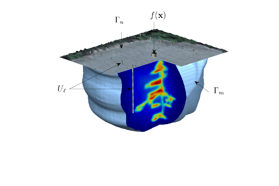
Figure 2: Geophysical application problem setting. The current sources $f(x)$ are applied though the borehole electrodes yielding electrode potentials $U_{\ell}$. $\Gamma_{m}$ is the model termination boundary and $\Gamma_{n}$ is the upper surface of the model domain $B$.

The electric potential measurements are collected through point-wise electrodes, contact impedances of which are effectively zero. The measurement points are $\mathbf{x}_{\ell}$ for $\ell=1,2,\ldots,L$ and the measured potential at every point is

$$U_{\ell}=\int_{B}\mathrm{d}x\;u(\mathbf{x})\delta(\mathbf{x}-\mathbf{x}_{\ell}),$$ (32)

where $\delta(.)$ denotes the Dirac delta function. Consider a perturbation $\gamma\rightarrow\gamma+\delta\gamma$ in the additivity causing the potential perturbation $u\rightarrow u+\delta u$. Introducing these into (30)–(31) gives

$$\nabla\cdot\big{(}(\gamma+\delta\gamma)\nabla(u+\delta u)\big{)} = f,\hskip 41.25641pt\mbox{on}\;B,$$ (33)

$$\alpha(\gamma+\delta\gamma)\nabla(u+\delta u)\cdot\mathbf{n}+\beta(u+\delta u) = 0,\hskip 41.25641pt\mbox{on}\;\partial B.$$ (34)

Expanding (32) and (33) and using (30)–(31) to simplify the resulting terms yields

$$\nabla\cdot(\delta\gamma\nabla u)+\nabla\cdot(\gamma\nabla\delta u)+\nabla\cdot(\delta\gamma\nabla\delta u) = 0,\hskip 41.25641pt\mbox{on}\;B,$$ (35)

$$\alpha(\delta\gamma\nabla u\cdot\mathbf{n}+\gamma\nabla\delta u\cdot\mathbf{n}+\delta\gamma\nabla\delta u\cdot\mathbf{n})+\beta\delta u = 0,\hskip 41.25641pt\mbox{on}\;\partial B.$$ (36)

Based on (32) a perturbation in the measurement at $\mathbf{x}_{\ell}$ can be written as a volume integral

$$\delta U_{\ell}=\int_{B}\mathrm{d}x\;\delta u(\mathbf{x})\delta(\mathbf{x}-\mathbf{x}_{\ell})$$ (37)

To proceed with finding a closed form for the measurement perturbation $\delta U_{\ell}$, it is useful to define $v$, as the solution to the adjoint system

$$\nabla\cdot(\overline{\gamma}\nabla v_{\ell}) = \delta(\mathbf{x}-\mathbf{x}_{\ell}),\hskip 41.25641pt\mathbf{x}\in B,$$ (38)

$$\alpha\overline{\gamma}\nabla v_{\ell}\cdot\mathbf{n}+\beta v_{\ell} = 0,\hskip 75.39963pt\mathbf{x}\in\;\partial B,$$ (39)

from which it is easily inferred that $\overline{v_{\ell}}$ satisfies

$$\nabla\cdot(\gamma\nabla\overline{v_{\ell}}) = \delta(\mathbf{x}-\mathbf{x}_{\ell}),\hskip 41.25641pt\mathbf{x}\in B,$$ (40)

$$\alpha\gamma\nabla\overline{v_{\ell}}\cdot\mathbf{n}+\beta\overline{v_{\ell}} = 0,\hskip 75.39963pt\mathbf{x}\in\;\partial B.$$ (41)

Using (37) and (40) we conclude that the perturbation to the residuals can be written in terms of the adjoint field as

$$\delta U_{\ell}=\int_{B}\mathrm{d}x\;\delta u(\mathbf{x})\;\nabla\cdot(\gamma\nabla\overline{v_{\ell}}).$$ (42)

The remaining derivation requires extensive use of the following identity derived from Green’s theorem [30] for vector function $\mathbf{\Psi}$ and scalar function $\psi$

$$\int_{B}\mathrm{d}x\,\mathbf{\Psi}\cdot\nabla\psi+\int_{B}\mathrm{d}x\,\psi\nabla\cdot\mathbf{\Psi}=\int_{\partial B}\mathrm{d}s\,\psi\mathbf{\Psi}\cdot\mathbf{n}.$$ (43)

We begin by taking $\psi=\delta u$ and $\mathbf{\Psi}=\gamma\nabla\overline{v_{\ell}}$ in (42) to obtain

$$\delta U_{\ell}=-\int_{B}\mathrm{d}x\,\gamma\nabla\overline{v_{\ell}}\cdot\nabla\delta u+\int_{\partial B}\mathrm{d}s\,\gamma\delta u\nabla\overline{v_{\ell}}\cdot\mathbf{n}.$$ (44)

Next using $\psi=\overline{v_{\ell}}$ and $\mathbf{\Psi}=\gamma\nabla\delta u$ in the first term on the right hand side of (44), we have

$$\delta U_{\ell}=\int_{B}\mathrm{d}x\,\overline{v_{\ell}}\nabla\cdot(\gamma\nabla\delta u)-\int_{\partial B}\mathrm{d}s\,\gamma\;\overline{v_{\ell}}\nabla\delta u\cdot\mathbf{n}+\int_{\partial B}\mathrm{d}s\,\gamma\delta u\nabla\overline{v_{\ell}}\cdot\mathbf{n}.$$ (45)

From (35), $\nabla\cdot(\gamma\nabla\delta u)=-\nabla\cdot(\delta\gamma\nabla u)-\nabla\cdot(\delta\gamma\nabla\delta u)$ which we use in the first term on the right hand side of (45) to arrive at

$$\delta U_{\ell}=-\int_{B}\mathrm{d}x\,\overline{v_{\ell}}\nabla\cdot\big{(}\delta\gamma\nabla(u+\delta u)\big{)}-\int_{\partial B}\mathrm{d}s\,\gamma\;\overline{v_{\ell}}\nabla\delta u\cdot\mathbf{n}+\int_{\partial B}\mathrm{d}s\,\gamma\delta u\nabla\overline{v_{\ell}}\cdot\mathbf{n}.$$ (46)

Appealing once more to (43) with $\psi=\overline{v_{\ell}}$ and $\mathbf{\Psi}=\delta\gamma\nabla(u+\delta u)$ in the first term of (46) gives

$$\delta U_{\ell} =\int_{B}\mathrm{d}x\,\delta\gamma\nabla\overline{v_{\ell}}\cdot\nabla u+\int_{B}\mathrm{d}x\,\delta\gamma\nabla\overline{v_{\ell}}\cdot\nabla\delta u$$

$$-\int_{\partial B}\mathrm{d}s\,\big{(}\gamma\overline{v_{\ell}}\nabla\delta u\cdot\mathbf{n}+\delta\gamma\overline{v_{\ell}}\nabla u\cdot\mathbf{n}+\delta\gamma\overline{v_{\ell}}\nabla\delta u\cdot\mathbf{n}-\gamma\delta u\nabla\overline{v_{\ell}}\cdot\mathbf{n}\big{)}.$$ (47)

We now show that the surface integral term in (47) is zero. For this purpose we multiply both sides of (41) by $\delta u$ to arrive at

$$\alpha\gamma\delta u\nabla\overline{v_{\ell}}\cdot\mathbf{n}+\beta\delta u\overline{v_{\ell}}=0$$ (48)

Using (36) to replace the term $\beta\delta u$ in (48) results in

$$-\alpha\big{(}\gamma\overline{v_{\ell}}\nabla\delta u\cdot\mathbf{n}+\delta\gamma\overline{v_{\ell}}\nabla u\cdot\mathbf{n}+\delta\gamma\overline{v_{\ell}}\nabla\delta u\cdot\mathbf{n}-\gamma\delta u\nabla\overline{v_{\ell}}\cdot\mathbf{n}\big{)}=0,\qquad\text{on}\;\partial B.$$ (49)

The parenthesized expression in (49) is the same as the surface integrand in (47). We partition the boundary $\partial B$ into $\Gamma_{\alpha}$ where $\alpha\neq 0$ and $\partial B\setminus\Gamma_{\alpha}$ where $\alpha=0$. Clearly (49) results the inside bracket expression to vanish on $\Gamma_{\alpha}$. On the remaining surface $\partial B\setminus\Gamma_{\alpha}$ that $\alpha=0$, we certainly have $\beta\neq 0$ since $\alpha$ and $\beta$ may not be simultaneously zero and using this fact in (36) and (41) would result in $\delta u=0$ and $\overline{v_{\ell}}=0$ which again make the inside bracket term zero. Therefore the surface integral in (47) vanishes both on $\Gamma_{\alpha}$ and $\partial B\setminus\Gamma_{\alpha}$ and therefore

$$\delta U_{\ell}=\int_{B}\mathrm{d}x\,\delta\gamma\nabla\overline{v_{\ell}}\cdot\nabla u+\int_{B}\mathrm{d}x\,\delta\gamma\nabla\overline{v_{\ell}}\cdot\nabla\delta u,$$ (50)

and thus by substituting for $\delta u$ in the second term we arrive at the result of the theorem 3.3.

4 High-order regularized regression

Within the $d-$ dimensional sphere $S_{\gamma_{p},\kappa}$, the electric potential field in the interior of the domain admits a Taylor expansion

$$u(\gamma)=u(\gamma_{p})+\partial_{\gamma}u(\gamma_{p})\delta\gamma+\mathcal{O}(\|\delta\gamma^{2}\|)$$

hence to first-order accuracy this can be approximated by

$$u(\gamma)\simeq\hat{u}(\gamma)=u(\gamma_{p})+\partial_{\gamma}u(\gamma_{p})\delta\gamma.$$ (51)

Introducing the right hand side of (51) in the integral equation (29) gives

$$\delta\zeta_{k} \approx -\int_{B}\mathrm{d}x\;\delta\gamma\nabla\bigl{(}u(\gamma_{p})+\partial_{\gamma}u(\gamma_{p})\delta\gamma\bigr{)}\cdot\nabla\overline{v}(\gamma_{p}),$$

$$= -\int_{B}\mathrm{d}x\;\delta\gamma\nabla u(\gamma_{p})\cdot\nabla\overline{v}(\gamma_{p})-\int_{B}\mathrm{d}x\;\delta\gamma\;\nabla(\partial_{\gamma}u(\gamma_{p})\delta\gamma)\cdot\nabla\overline{v}(\gamma_{p}),$$

where the first, linear term, involves the definition of the Fréchet derivative of the forward mapping as in (16) [2], [32], and the second nonlinear term the differential operator $\partial_{\gamma}u(\gamma_{p})$ that provides a measure on local sensitivity of the potential in the interior of the domain to perturbations in electrical properties. From (51), (4), it is trivial to deduce that the linear approximation of the forward operator $\mathcal{E}$ as in (15), as proposed by Calderón in [8], effectively imposes a zeroth-order Taylor approximation on the electric potential $\hat{u}(\gamma)\simeq u(\gamma_{p})$. In turn this enforces $\partial_{\gamma}u$ and higher-order derivatives to vanish everywhere in $\bar{B}$, thus elliminating the nonlinear terms in (28) and (4). Let the linear operator $\partial_{\gamma}\mathcal{E}=\mathcal{J}:L^{\infty}(\overline{B})\rightarrow\mathbb{C}^{m}$, and nonlinear, quadratic in $\delta\gamma$, $\mathcal{K}:L^{\infty}(\overline{B})\rightarrow\mathbb{C}^{m}$ defined by

$$\mathcal{J}\,\delta\gamma \doteq -\int_{B}\mathrm{d}x\;\delta\gamma\;\nabla u(\gamma_{p})\cdot\nabla\overline{v}(\gamma_{p}),$$ (53)

$$\mathcal{K}\,\delta\gamma \doteq -\int_{B}\mathrm{d}x\;\delta\gamma\;\nabla\partial_{\gamma}u(\gamma_{p})\delta\gamma\cdot\nabla\overline{v}(\gamma_{p})$$ (54)

then the inverse problem can be formulated in the context of regularized regression based on the nonlinear operator equation

$$\delta\zeta=\mathcal{J}\delta\gamma+\mathcal{K}\delta\gamma+\eta.$$ (55)

4.1 Numerical approximation

Usually the EIT problem is approached with a numerical approximation method like finite elements, where the governing equations are discretized on a finite dimensional model of the domain, say $B_{h}(n,N)$ comprising $n$ nodes connected in $N$ elements [37]. For simplicity in the notation we assume linear Lagrangian finite elements and consider element-wise linear and constant basis functions for the support of the electric potential $u$ and conductivity $\gamma$ respectively,

$$u(\mathbf{x},\omega)=\sum_{i=1}^{n}u_{i}\phi_{i},\quad\phi_{i}:B_{h}\rightarrow\mathbb{R},\qquad\gamma(\mathbf{x},\omega)=\sum_{i=1}^{N}\gamma_{i}\chi_{i},\quad\chi_{i}:B_{h}\rightarrow\mathbb{R}$$ (56)

where $\{\phi_{i}\}_{i=1}^{n}$ and $\{\chi_{i}\}_{i=1}^{N}$ the respective bases in $B_{h}$. Following the discretization of the domain into a finite number of elements, the basis functions $\{\phi_{1},\ldots,\phi_{n}\}$ in the expansion of the potential are assumed to belong in a finite, $n$-dimensional subspace of $H_{o}^{1}(B)$. For clarity in the notation, we keep $u$ and $\gamma$ as the vectors of coefficients relevant to the respective functions as from now on we deal exclusively the numerical approximation of the problem. On the discrete domain the weak form of the operator equation (55) is approximated by

$${\delta\zeta}_{k}=j_{k}^{\prime}\delta\gamma+{\delta\gamma}^{\prime}\mathbf{K}^{k}\delta\gamma+\eta_{k},\qquad k=1,\ldots,m$$ (57)

where $\zeta_{k}\in\mathbb{C}$ is the $k$th measurement, $j_{k}$ the $k$th row of the Jacobian matrix $\mathbf{J}$ that is the discrete form of $\partial_{\gamma}\mathcal{E}(\gamma_{p})$, $\mathbf{K}^{k}\in\mathbb{C}^{N\times N}$ is the $k$th coefficients (Hessian) matrix derived from $\mathcal{K}$ in (54), $\eta_{k}$ the noise in the $k$th measurement and $\delta\gamma\in\mathbb{C}^{N}$ the required perturbation in the admittivity coefficients. Let the additive noise be uncorrelated zero-mean Gaussian with diagonal covariance matrix $\mathbf{C}_{\eta}$, with positive diagonal element $c_{k}$ then the data misfit function

$$Q(\delta\gamma)=\sum_{k=1}^{m}c_{k}^{-1}\bigl{(}{\delta\zeta}_{k}-j_{k}^{\prime}\delta\gamma-\delta\gamma^{\prime}\mathbf{K}^{k}\delta\gamma\bigr{)}^{2}$$ (58)

can be used to define the regularized quadratic regression problem

$${\delta\gamma}^{*}=\arg\min_{\delta\gamma\in\mathbb{C}^{N}}\xi(\delta\gamma),\qquad\xi(\delta\gamma)\doteq\frac{1}{2}\bigl{\{}Q(\delta\gamma)+\alpha\mathcal{G}(\delta\gamma)\bigr{\}}$$ (59)

with $\mathcal{G}:\mathbb{C}^{N}\rightarrow\mathbb{R}$ a convex differentiable regularization term. On the other hand, choosing to neglect the matrices $\mathbf{K}^{k}$ yields the conventional misfit function

$$\Lambda(\delta\gamma)=\sum_{k=1}^{m}c_{k}^{-1}\bigl{(}{\delta\zeta}_{k}-j_{k}^{\prime}\delta\gamma\bigr{)}^{2},$$ (60)

often used in the context of regularized linear regression formulations. As shown in [1] the Jacobian matrix can be computed directly from (53) and (56) using numerical integration as

$$\mathbf{J}_{k,j}=-\int_{B_{j}}\mathrm{d}x\;\chi_{j}\;\sum_{l\,\in\,\mathrm{supp}(B_{j})}u_{l}\nabla\phi_{l}\sum_{l\,\in\,\mathrm{supp}(B_{j})}\overline{v}_{l}\nabla\phi_{l},\quad k=1,\ldots,m,\;j=1,\ldots,N$$ (61)

with $v$ the coefficients of the adjoint field solution corresponding to the $k$th measurement, and $\mathrm{supp}(B_{j})$ the support of the $j$th element. To derive the respective element of $\mathbf{K}^{k}$ we follow an approach similar to that of Kaipio et al. in [21] that is based on the Galerkin formulation of the problem. For this we choose $\{\phi_{1},\ldots,\phi_{n}\}$ as a test basis for the potentials and by substituting into the variational form of the model we arrive at

$$\sum_{i=1}^{n}\sum_{j=1}^{n}\Bigl{(}\int_{B}\mathrm{d}x\,\gamma\nabla\phi_{i}\cdot\nabla\phi_{j}+\sum_{\ell=1}^{L}z_{\ell}\int_{\Gamma_{e_{\ell}}}\mathrm{d}s\,\phi_{i}\,\phi_{j}\Bigr{)}u_{i}-\sum_{\ell=1}^{L}z_{\ell}\int_{\Gamma_{e_{\ell}}}\mathrm{d}s\,\phi_{i}\;U_{\ell}=0.$$

Imposing the Neumann conditions for the applied boundary currents yields the additional equations

$$I_{\ell}=-z_{\ell}\sum_{i=1}^{n}\Bigl{(}\int_{\Gamma_{e_{\ell}}}\mathrm{d}s\,\phi_{i}\Bigr{)}u_{i}+z_{\ell}\,|\Gamma_{e_{\ell}}|\,U_{\ell},\quad\ell=1,\ldots,L,$$

with $|\Gamma_{e_{\ell}}|$ the area of the $\ell$th electrode. In matrix form the electric potential expansion coefficients $u\in\mathbb{C}^{n}$ and the electrode potentials $U\in\mathbb{C}^{L}$ can be computed by solving the $(n+L)\times(n+L)$ matrix equation

$$\left[\begin{array}[]{c c}\mathbf{A}_{11}&\mathbf{A}_{12}\\ \mathbf{A}_{12}^{\prime}&\mathbf{A}_{22}\end{array}\right]\left[\begin{array}[]{c}u\\ U\end{array}\right]=\left[\begin{array}[]{c}0\\ I\end{array}\right],$$ (62)

where

$${\mathbf{A}_{11}}_{\,i,j} = \int_{B}\mathrm{d}x\,\gamma\nabla\phi_{i}\cdot\nabla\phi_{j}+\sum_{\ell=1}^{L}z_{\ell}\int_{\Gamma_{e_{\ell}}}\mathrm{d}s\,\phi_{i}\,\phi_{j},\quad i,j=1,\ldots,n$$

$${\mathbf{A}_{12}}_{\,i,\ell} = -z_{\ell}\int_{\Gamma_{e_{\ell}}}\mathrm{d}s\,\phi_{i},\quad i=1,\ldots,n,\quad\ell=1,\ldots,L,$$

$${\mathbf{A}_{22}}_{\,\ell,\ell} = z_{\ell}|\Gamma_{e_{\ell}}|,\quad\ell=1,\ldots,L.$$

For a conductivity $\gamma$ and applied current $I$, let $\begin{bmatrix}u\\ U\end{bmatrix}=\mathbf{A}^{-1}(\gamma)\begin{bmatrix}0\\ I\end{bmatrix}$ the solution of (62). Using the matrix differentiation formula, the partial derivatives with respect to the $q$th admittivity element are

$$\partial_{\gamma_{q}}\begin{Bmatrix}u\\ U\end{Bmatrix}=\frac{\partial}{\partial_{\gamma_{q}}}\begin{Bmatrix}\mathbf{A}^{-1}(\gamma)\begin{bmatrix}0\\ I\end{bmatrix}\end{Bmatrix} = -\mathbf{A}^{-1}(\gamma)\,\partial_{\gamma_{q}}\bigl{\{}\mathbf{A}(\gamma)\bigr{\}}\,\mathbf{A}^{-1}(\gamma)I$$

$$= -\mathbf{A}^{-1}(\gamma)\,\partial_{\gamma_{q}}\bigl{\{}\mathbf{A}(\gamma)\bigr{\}}\,\begin{bmatrix}u\\ U\end{bmatrix},$$

where

$$\partial_{\gamma_{q}}\bigl{\{}\mathbf{A}(\gamma)\bigr{\}}=\partial_{\gamma_{q}}\bigl{\{}\mathbf{A}_{11}(\gamma)\bigr{\}}=\int_{B_{q}}\mathrm{d}x\,\nabla\phi_{i}\cdot\nabla\phi_{j},\quad q=1,\ldots,N,$$

as only the block $\mathbf{A}_{11}$ depends on admittivity. Separating the above as

$$\partial_{\gamma_{q}}\begin{Bmatrix}u\\ U\end{Bmatrix}=\left[\begin{array}[]{c|c}\partial_{\gamma_{q}}u&\partial_{\gamma_{q}}U\end{array}\right]^{\prime}$$

and evaluating the upper part for all elements in the model yields the required matrix in vector concatenation form

$$\partial_{\gamma}u(\gamma)=\bigl{[}\begin{array}[]{c|c|c|c}\partial_{\gamma_{1}}u(\gamma)&\partial_{\gamma_{2}}u(\gamma)&\ldots&\partial_{\gamma_{N}}u(\gamma)\end{array}\bigr{]},$$ (63)

while $\partial_{\gamma_{q}}U$ are the elements of the Jacobian matrix $\mathbf{J}$. Effectively the element of $\mathbf{K}^{k}$ matrix is given by

$$\mathbf{K}^{k}_{r,j}=-\int_{B_{j}}\mathrm{d}x\;\psi_{j}\;\sum_{l\in\mathrm{supp}(B_{r})}\nabla\phi_{l}\;\partial_{\gamma_{r}}u_{l}\sum_{l\,\in\,\mathrm{supp}(B_{j})}\overline{v}_{l}\nabla\phi_{l},\quad k=1,\ldots,m,\;\,r,j=1,\ldots,N$$

with $v$ the adjoint field corresponding to the $k$th measurement and $\partial_{\gamma_{r}}u$ the derivative of the $k$th direct field with respect to $\gamma_{r}$.

4.2 Newton’s minimization method

We propose solving the regularized problem (59) using Gauss-Newton’s minimization method [18]. At a feasible point $\delta\gamma_{p}$ the minimization cost function $\xi$ is approximated by a second-order Taylor series [16]

$$\hat{\xi}(\delta\gamma)=\xi(\delta\gamma_{p})+\partial_{\delta\gamma}\xi(\delta\gamma_{p})(\delta\gamma-\delta\gamma_{p})+\frac{1}{2}(\delta\gamma-\delta\gamma_{p})^{\prime}\partial_{\delta\gamma\delta\gamma}\xi(\delta\gamma_{p})(\delta\gamma-\delta\gamma_{p}),$$ (64)

where applying first-order optimality conditions $\partial_{\delta\gamma}\hat{\xi}(\delta\gamma)=0$ yields the linear system

$$\partial_{\delta\gamma}\hat{\xi}(\delta\gamma_{p})=-\partial_{\delta\gamma\delta\gamma}\hat{\xi}(\delta\gamma_{p})(\delta\gamma-\delta\gamma_{p}).$$

From (58), let the $k$th residual function be

$$r_{k}(\delta\gamma)=c_{k}^{-1/2}\Bigl{(}{\delta\zeta}_{k}-\sum_{j=1}^{N}\mathbf{J}_{k,j}\delta\gamma_{j}-\sum_{j=1}^{N}\delta\gamma_{j}\sum_{l=1}^{N}\mathbf{K}^{k}_{j,l}\delta\gamma_{l}\Bigr{)},$$

such that $Q(\delta\gamma)=\|r(\delta\gamma)\|^{2}$, then the cost gradient $\partial_{\delta\gamma}\hat{\xi}(\gamma_{p})$ and Hessian $\partial_{\delta\gamma\delta\gamma}\hat{\xi}(\delta\gamma_{p})$ are expressed as

$$\partial_{\delta\gamma}\hat{\xi}(\delta\gamma_{p}) = \partial_{\delta\gamma}r(\delta\gamma_{p})^{\prime}r(\delta\gamma_{p})+\alpha\mathbf{C}_{\gamma}^{-1}\delta\gamma_{p},$$

$$\partial_{\delta\gamma\delta\gamma}\hat{\xi}(\delta\gamma_{p}) = \partial_{\delta\gamma}r(\delta\gamma_{p})^{\prime}\partial_{\delta\gamma}r(\delta\gamma_{p})+\alpha\mathbf{C}_{\gamma}^{-1}$$

for $r(\delta\gamma)=\begin{bmatrix}r_{1}(\delta\gamma),&\ldots,&r_{m}(\delta\gamma)\end{bmatrix}^{\prime}$, and assuming a Tikhonov-type regularization function $\mathcal{G}(\delta\gamma)=\alpha{\delta\gamma}^{\prime}\mathbf{C}_{\gamma}^{-1}\delta\gamma$, with $\mathbf{C}_{\gamma}^{-1}$ positive semidefinite and $\alpha$ a positive regularization parameter. The Jacobian of the residual $\partial_{\delta\gamma}r(\partial\gamma_{p})\in\mathbb{C}^{m\times N}$ is then formed using the vectors

$$\partial_{\delta\gamma_{l}}r_{k}(\delta\gamma)=-c_{k}^{-1/2}\mathbf{J}_{k,l}-c_{k}^{-1/2}\sum_{j=1}^{N}\Bigl{(}\mathbf{K}^{k}_{l,j}+\mathbf{K}^{k}_{j,l}\Bigr{)}\delta\gamma_{j},\quad l=1,\ldots,N,$$

evaluated at $\delta\gamma_{p}$ like

$$\partial_{\delta\gamma}r(\delta\gamma_{p})=\begin{bmatrix}\partial_{\delta\gamma}r_{1}(\delta\gamma_{p})&|&\partial_{\delta\gamma}r_{2}(\delta\gamma_{p})&|&\ldots&|&\partial_{\delta\gamma}r_{m}(\delta\gamma_{p})\end{bmatrix}^{\prime}.$$

If $\partial_{\delta\gamma\delta\gamma}\hat{\xi}(\delta\gamma_{p})$ is full rank and positive definite the solution can be computed iteratively using Newton’s algorithm

$$\delta\gamma_{p+1}=\delta\gamma_{p}-\partial_{\delta\gamma\delta\gamma}^{-1}\hat{\xi}(\delta\gamma_{p})\,\partial_{\delta\gamma}\hat{\xi}(\delta\gamma_{p}),\qquad p=0,1,2,\ldots$$ (65)

Using standard arguments from the convergence analysis of Newton’s method on convex minimization it is easy to show convergence as in [18], [27]

$$\hat{\xi}(\delta\gamma_{p})>\hat{\xi}(\delta\gamma_{p+1})\geq\|\eta\|,\quad\|\delta\gamma^{*}-\delta\gamma_{p}\|\geq\|\delta\gamma^{*}-\delta\gamma_{p+1}\|,\quad p=0,1,\ldots,$$ (66)

however a convergence in the sense of the discrepancy principle is more appropriate as the data are likely to contain noise [22].

Corollary 4.1

Initializing the quadratic regression iteration (65) with $\delta\gamma_{0}=0$ yields a first iteration that coincides with the linear regularized regression estimator

$$\delta\gamma_{1}=\bigl{(}\mathbf{J}^{\prime}\mathbf{C}_{\eta}^{-1}\mathbf{J}+\alpha\mathbf{C}_{\gamma}^{-1}\bigr{)}^{-1}\mathbf{J}^{\prime}\mathbf{C}_{\eta}^{-1}\delta\zeta$$ (67)

• The proof is by substitution of the residual and its Jacobian at $\delta\gamma_{0}=0$ into the expressions for the gradient and Hessian of the cost function. In particular for $r(\delta\gamma_{0})=\mathbf{C}_{\eta}^{-1/2}\delta\zeta$ and $\partial_{\delta\gamma}r(\delta\gamma_{0})=\mathbf{C}_{\eta}^{-1/2}\mathbf{J}$, iteration (65) yields the result.

Combining the convergence remarks of (66) with the corollary above, we assert that for $p>1$ the quadratic regression iterations should converge in a solution whose error does not exceed that of the linear regression problem (17). Suppose now that at a certain iteration $p$ the value of the residual $r(\delta\gamma_{p})$ converges to the level of noise $\|\eta\|$. Then according to the discrepancy principle one updates the admittivity estimate as $\gamma_{p+1}=\gamma_{p}+\delta\gamma_{p}$ and thereafter the definitions of $\mathbf{J}$ and $\mathbf{K}^{k}$, and then proceeds to the next iteration. Effectively, the resulting scheme can be expressed as a Newton-type algorithm.

1. Given data $\zeta\in\mathbb{C}^{m}$ with noise level $\|\eta\|$ and a finite domain $B_{h}$ with unknown admittivity $\gamma^{*}\in\mathbb{C}^{N}$

2. Set $q=0$, choose initial admittivity distribution $\gamma_{0}$,

3. For $q=1,2,\ldots\quad$ (Exterior iterations)

4. Compute data $\delta\zeta=\zeta-\mathcal{E}(\gamma_{q-1})$, and matrices $\mathbf{J}\in\mathbb{C}^{m\times N}$, $\mathbf{K}^{k}\in\mathbb{C}^{N\times N}$, for $\gamma_{q-1}$, and $k=1,\ldots,m$,

   1. Set $p=0$, $\delta\gamma_{p}=0$,

   2. For $p=1,2,\ldots\quad$ (Interior iterations)

   3. Compute update

      $$\delta\gamma_{p}=\delta\gamma_{p-1}-\tau_{p}\partial_{\delta\gamma\delta\gamma}^{-1}\hat{\xi}(\delta\gamma_{p-1})\,\partial_{\delta\gamma}\hat{\xi}(\delta\gamma_{p-1}),\;\tau_{p}>0,$$

   4. End $p$ iterations

   5. Compute update

      $$\gamma_{q}=\gamma_{q-1}+\tau_{q}\delta\gamma_{p},\;\tau_{q}>0,$$

5. End $q$ iterations

In performing the outer iterations, a complication will likely arise in that a certain update admittivity change $\delta\gamma_{p}$ may cause the real and/or imaginary components of $\gamma_{q+1}$ to become zero or negative. This of course violates a physical restriction on the electrical properties of the media, and the solution cannot be admitted. For this reason the problem of (59) should be posed as a linearly constrained problem

$${\delta\gamma}^{*}=\arg\min_{\gamma_{q}>\delta\gamma}\xi(\delta\gamma),$$

at each $\gamma_{q}$. A convenient heuristic to prevent this complication is by adjusting the step sizes $\tau_{q},\tau_{p}$ until the above inequality is satisfied [37], [43]. Note also, that the above methodology makes no explicit assumptions on the type of the regularization functional $\mathcal{G}(\gamma)$, aside its differentiability, thus we anticipate it can be also be implemented in conjunction with total variation and $\ell_{1}$-type regularization [7] as well as the level sets method [11].

5 Numerical results

To test the performance of the proposed algorithm we perform some numerical simulations using two-dimensional models, although the extension to three dimensions follows in a trivial way. In this context we consider a rectangular domain $B=[-16,16]\times[0,-32]\subset\mathbb{R}^{2}$, with $L=30$ point electrodes attached at its boundary in a borehole and surface arrangement as shown in figures 6 and 7. As a first test case the domain is assumed to have an unknown target conductivity $\gamma^{*}$ whose real and imaginary components are functions with respective bounds $1.46\leq\sigma^{*}\leq 5.60$ and $0.74\leq\omega\epsilon^{*}\leq 3.90$. To compute the measurements we consider 15 pair drive current patterns $I^{d}$, $d=1,\ldots,L/2$, yielding a vector of $m=390$ linearly independent voltage measurements $\zeta\in\mathbb{C}^{m}$. The forward problem is approximated using the finite element method outlined in the previous section, and to the measurements we add a Gaussian noise signal of zero mean and positive definite covariance matrix $\mathbf{C}_{\eta}=10^{-5}\max|\zeta|\,\mathbf{I}$, where $\mathbf{I}$ is the identify matrix. For the forward problem we use a finite dimensional model $B_{f}$ comprising $n=1701$ nodes connected in $N=3144$ linear triangular elements. All other computations are performed on a coarser grid $B_{i}$ with $n=564$ nodes and $N=1038$ elements. The two finite models are nested, hence for any function $\gamma$ approximated on $B_{i}$ with expansion coefficients $\gamma_{i}$ there exists a projection $\gamma_{f}=\Pi\gamma_{i}$, mapping it onto $B_{f}$. To reconstruct the synthetic data we assume an initial homogeneous admittivity model $\gamma_{0}=3.90+2.40i$ which coincides with the mean value of $\gamma^{*}$, a methodology adopted from [19].

At the initial admittivity guess $\gamma_{0}$ we approximate the potential $u(\gamma^{*})$ using the zeroth-order and first-order Taylor series $u(\gamma_{0})$ and $u(\gamma_{0})+\partial_{\gamma}u(\delta\gamma_{0})(\gamma-\gamma_{0})$ respectively. The normalized approximation errors are illustrated at the top of figure 3 next to those of the error in the induced potential gradient as this is involved in the computation of the $\mathbf{K}^{k}$ matrices for $k=1,\ldots,390$. The results show that the linear approximation sustains a smaller error in both quantities and at all applied current patterns. In the same figure we also plot the measurement perturbations $\delta\zeta=\zeta-\mathcal{E}(\gamma_{0})$ versus the linear and the quadratic predictions to demonstrate that the proposed quadratic regression will fit the noisy measurements at a smaller error. In particular, the quadratic and linear misfit cost functions in (58) and (60) are evaluated at $Q(\delta\gamma_{0})=0.06$ and $\Lambda(\delta\gamma_{0})=0.13$, where $\delta\gamma_{0}=\gamma^{*}-\gamma_{0}$. Notice the impact of the second-order term, that brings the norm of the data misfit to about half of that of the linear case.

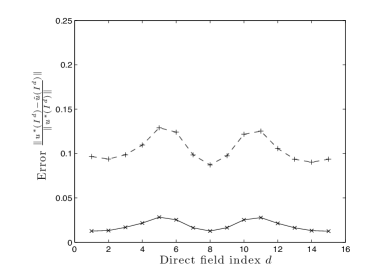
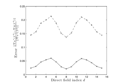
Figure 3: At the top row, the normalized errors in the electric potential field approximation and its gradient, assuming zeroth-order (dashed line with $+$ markers) and first-order (solid line with $\times$ markers) Taylor series approximations of $u(\gamma^{*},I^{d})$ direct fields. In both cases the errors with the linear approximation are lower. Second row, the quality of the linear and quadratic approximations in predicting the nonlinear change in the boundary data $\delta\zeta$. The solid line denotes $\delta\zeta_{i}$, the dashed $j_{i}^{\prime}\delta\gamma$ and the dotted $j_{i}^{\prime}\delta\gamma+\sum_{i=1}^{m}\delta\gamma^{\prime}\mathbf{K}^{i}\delta\gamma$, over the interval $i=150,\ldots,220$. The corresponding data misfit norms are $0.057$ for the quadratic approximation $Q(\delta\gamma^{*})$ and $0.123$ for the linear $\Lambda(\delta\gamma^{*})$, assuming no additive noise. With the prescribed additive noise these values change to $0.062$ and $0.126$ respectively.

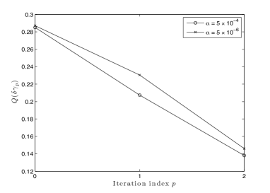
Figure 4: Indicative convergence of the proposed method, in terms of minimizing the quadratic misfit error $Q(\delta\gamma_{p})$ for two different values of the regularization parameter $\alpha$. Left the results during the first exterior iteration $q=1$, and right the corresponding values for $q=2$. In these results, $\delta\gamma_{0}=0$, $\delta\gamma_{1}$ coincides with the Tikhonov solution, and $\delta\gamma_{2}$ is the regularized quadratic regression solution. Notice that the quadratic regression solution has lower data misfit errors in both GN iterations. Between the first and second exterior iteration the admittivity increment was scaled to preserve positivity, hence the apparent discontinuity in the error reduction.

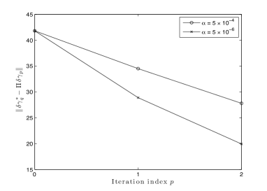
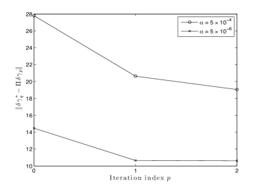
Figure 5: Indicative convergence of the proposed method, in terms of minimizing the the image error $\|\delta\gamma_{q}^{*}-\Pi\delta\gamma_{p}\|$ for two different values of the regularization parameter $\alpha$. Left the results during the first exterior iteration $q=1$, and right the corresponding values for $q=2$. In these figures $\delta\gamma_{0}=0$, $\delta\gamma_{1}$ coincides with the Tikhonov solution, and $\delta\gamma_{2}$ is the regularized quadratic regression solution. Notice that the quadratic regression solution maintains lower image errors at each external iteration. Between the first and second exterior iteration the admittivity increment was scaled to preserve positivity, hence the apparent discontinuity in the error reduction.

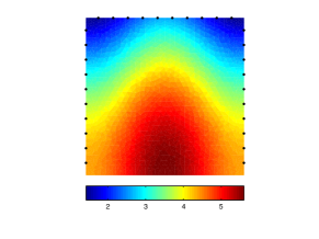
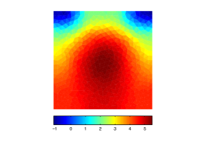
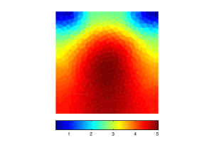
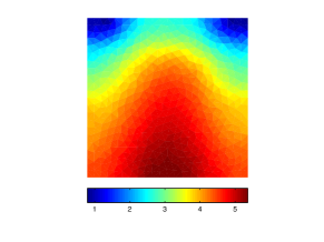
Figure 6: At the top, the simulated target conductivity $\sigma^{*}$ profile on $B_{f}$, as used in the first test example and the arrangement of the electrodes. In the second row, from left to right, the respective images resulted from first exterior iteration using $\alpha=5\times 10^{-6}$, namely the real components of $\gamma_{0}+\tau\delta\gamma_{1}$, $\gamma_{0}+\tau\delta\gamma_{2}$, and $\gamma_{1}$ on $B_{i}$. Similarly at the bottom row, the respective images from the second exterior GN iteration, $\gamma_{1}+\tau\delta\gamma_{1}$, $\gamma_{1}+\tau\delta\gamma_{2}$, and $\gamma_{2}$, using the same value of $\alpha$.

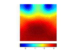
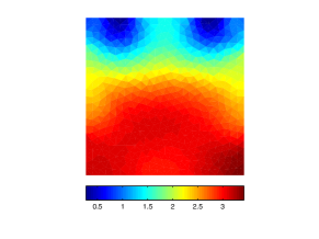
Figure 7: At the top, the simulated target scaled permittivity $\omega\epsilon^{*}$ profile on $B_{f}$, as used in the first test example and the arrangement of the electrodes. In the second row, from left to right, the respective images resulted from first exterior iteration using $\alpha=5\times 10^{-6}$, namely the imaginary components of $\gamma_{0}+\tau\delta\gamma_{1}$, $\gamma_{0}+\tau\delta\gamma_{2}$, and $\gamma_{1}$ on $B_{i}$. Similarly at the bottom row, the respective images from the second exterior GN iteration, $\gamma_{1}+\tau\delta\gamma_{1}$, $\gamma_{1}+\tau\delta\gamma_{2}$, and $\gamma_{2}$, using the same value of $\alpha$.

To reconstruct the admittivity function we implement the proposed iteration (65) using a precision matrix $\mathbf{C}^{-1}_{\gamma}=\mathbf{R}^{\prime}\mathbf{R}$, where $\mathbf{R}\in\mathbb{R}^{N\times N}$ is a smoothness enforcing operator. In the numerical experiments we use two different values of the regularization parameter in order to investigate the performance of the scheme at different levels of regularization. Using $\alpha=5\times 10^{-4}$ and $\alpha=5\times 10^{-6}$, we execute two exterior GN iterations each one incorporating two inner Newton iterations after which the algorithm converged to an error value just above the noise level. The error reduction is illustrated by the graphs of figures 4 and 5, showing a significant reduction in both the misfit error $Q(\delta\gamma_{p})$ and the image error $\|\delta\gamma_{q}^{*}-\Pi\delta\gamma_{p}\|$ respectively for $p=0,1,2$ for the first and second GN iterations, i.e. $q=1,2$. Each exterior iteration was initialized with $\delta\gamma_{0}=0$ hence we can regard $\delta\gamma_{1}$ as the Tikhonov solution (67) and $\delta\gamma_{2}$ the quadratic regressor after two iterations (65). To aid convergence a backtracking line search algorithm was used where the optimal step sizes for each iteration, interior and exterior. The computational time required to assemble the Jacobians $\mathbf{J}\in\mathbb{C}^{390\times 1038}$ was about 0.34 s, while each of the 390 matrices $\mathbf{K}^{k}\in\mathbb{C}^{1038\times 1038}$ took about 4.75 s and then each iteration about 12 s depending on the line search. These times are based on running Matlab [31] on a machine with a dual core processor at 2.53 GHz. Despite the substantial computational overhead, the method can be appealing in the cases where the inverse problem is heavily underdetermined with only a few measurements. Moreover, the assembling of the $\mathbf{K}$ matrices is well suited for parallel processing. The images of the reconstructed admittivity perturbation at each iteration are plotted in figures 6 (real component) and 7 (imaginary component) below their respective target images for comparison. As the error graphs clearly indicate, the reconstructed images show a profound quantitative improvement in spatial resolution, with the regularized quadratic regression solution $\delta\gamma_{2}$ to outperform the Tikhonov solution $\delta\gamma_{1}$ in both Gauss-Newton iterations. Notice however, that in the exterior iteration we scaled the increment $\delta\gamma_{p}$ by $\tau_{q}$ in order to preserve the positivity new admittivity estimate. This scaling, if $\tau_{q}<1$ tends to increase the data misfit errors, hence one can observe some discontinuities in the error reduction from $q=1$ to $q=2$ in the plots of figure 4. Similarly for the graphs of the image error in figure 5, although this time the correction works out to the improvement of the errors as the target images are by definition positive. For completeness, the step sizes used in the image reconstructions of figures 6 and 7 are $\tau_{p=1}=1$, $\tau_{p=2}=0.3$, and $\tau_{q=1}=0.78$ for the first cycle of iterations and $\tau_{p=1}=1$, $\tau_{p=2}=0.38$, and $\tau_{q=1}=1$ for the second.

As a second example we consider a purely conductive case, i.e. $\omega=0$, aiming to reconstruct the target conductivity function appearing at the top of figure 10. Once again synthetic data are simulated, using the same current and measurement patterns as in the previous case. After computing the measurements $\zeta$ and introducing some zero mean Gaussian noise using the noise covariance covariance matrix $\mathbf{C}_{\eta}=10^{-5}\max|\zeta|\,\mathbf{I}$ we formulate the inverse problem at a homogeneous background conductivity $\sigma_{0}$, the best homogeneous fit of the data, regularization matrix $\mathbf{R}$, and $\alpha$ parameters equal to $10^{-5}$ and $10^{-7}$. To aid comparison with the convergent results for the complex admittivity case we implement the algorithm for two interior and two exterior iterations, for each of the regularized problems. The graphs of the data misfit and image errors are illustrated in figures 8 and 9. The graphs show a convergence pattern similar to that of the complex case, for both values of the regularization parameter. Also at the initial reference point the linear and quadratic data misfit functions obtain values $\Lambda(\delta\sigma_{0})=0.24$ and $Q(\delta\sigma_{0})=0.09$, demonstrating once again that the contribution of the quadratic term can be significant if the reference point is not sufficiently close to the solution. In terms of its computational cost, implementing the algorithm for the purely real admittivity has brought the processing time to about a half of that consumed for the complex case. The reconstructed images presented in figure 10, correspond to the various conductivity updates as computed for two exterior and two interior iterations, with $\alpha=10^{-7}$. Initializing with $\delta\sigma_{0}=0$ the second row, from left to right, shows the conductivity updates after each interior iteration for the first exterior GN iteration, and the bottom row the respective images from the second exterior iteration. The step sizes used in these results, as computed by the line search algorithms are $\tau_{p=1}=1$, $\tau_{p=2}=0.3$, and $\tau_{q=1}=0.62$ for the first cycle of iterations and $\tau_{p=1}=0.62$, $\tau_{p=2}=0.24$, and $\tau_{q=1}=1$ for the second. Moreover at the beginning of the second GN iteration the misfit functions have been computed at $\Lambda(\delta\sigma_{1})=0.034$ and $Q(\delta\sigma_{1})=0.007$.

When the noise level in the data is approximately known, solving the nonlinear EIT problem one typically performs a number of GN iterations until convergence is reached in the sense of the discrepancy principle [27], [43]. In our results we implement only two exterior GN iterations, i.e. $q=1,2$, each one encompassing two interior iterations, in order to demonstrate the observed reduction in the image and data misfit errors. Consequently, by virtue of the convergence properties of the Newton algorithm, it is straightforward to state that the quadratic regression solution will sustain a smaller error for any number of GN iterations [3], and will thus converge to the solution faster. On the other hand, a serious bottleneck of the second, respectively higher-order, formulation is the computational demand to compute the $\mathbf{K}$ matrices. In this sense the method is more suited to the cases where high performance computing is available, or when the number of data $m$ is fairly small.

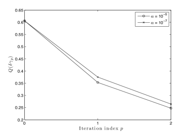
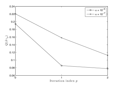
Figure 8: Indicative convergence of the proposed method, in terms of minimizing the quadratic misfit error $Q(\delta\gamma_{p})$ for two different values of the regularization parameter $\alpha$. Results are from the second test case with simulations at dc conditions $\omega=0$, hence the admittivity is purely real, i.e. $\gamma=\sigma$. Left the results during the first exterior iteration $q=1$, and right the corresponding values for $q=2$. In these results, $\delta\gamma_{0}=0$, $\delta\gamma_{1}$ coincides with the Tikhonov solution, and $\delta\gamma_{2}$ is the regularized quadratic regression solution. Notice that the quadratic regression solution has lower data misfit errors in both GN iterations. Between the first and second exterior iteration the admittivity increment was scaled to preserve positivity, hence the apparent discontinuity in the error reduction.

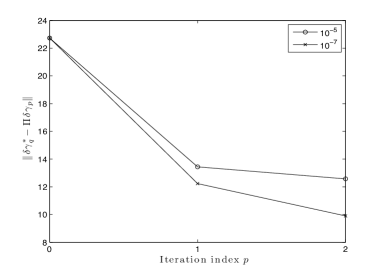
Figure 9: Indicative convergence of the proposed method, in terms of minimizing the the image error $\|\delta\gamma_{q}^{*}-\Pi\delta\gamma_{p}\|$ at each interior iteration for two different values of the regularization parameter $\alpha$. Results are from the second test case with simulations at dc conditions $\omega=0$, hence the admittivity is purely real, i.e. $\gamma=\sigma$. Left the results during the first exterior iteration $q=1$, and right the corresponding values for $q=2$. In the figures $\delta\gamma_{0}$ is the initial homogeneous guess, $\delta\gamma_{1}$ coincides with the Tikhonov solution, and $\delta\gamma_{2}$ is the regularized quadratic regression solution. Between the first and second exterior iteration the admittivity increment was scaled to preserve positivity, hence the apparent discontinuity in the error reduction.

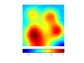
Figure 10: Simulated and reconstructed admittivity functions, for the second test case at direct current conditions. Top row, the target simulated conductivity $\sigma^{*}$ discretized in $B_{f}$. Below from first exterior iteration using $\alpha=10^{-7}$, namely $\sigma_{0}+\tau\delta\sigma_{1}$ , $\sigma_{0}+\tau\delta\sigma_{2}$, and $\sigma_{1}$ on $B_{i}$. Similarly at the bottom row, the respective images from the second exterior GN iteration, $\sigma_{1}+\tau\delta\sigma_{1}$, $\sigma_{1}+\tau\delta\sigma_{2}$, and $\sigma_{2}$, using the same value of $\alpha$.

6 Conclusions

This paper proposes a new approach for the inverse impedance tomography problem. Based on a a power perturbation approach we derive a nonlinear integral transform relating changes in electrical admittivity to those observed in the respective boundary measurements. This transform was then modified by assuming that the electric potential in the interior of a domain with unknown electrical properties can be approximated by a first-order Taylor expansion centered at an a priori admittivity estimate. This framework yields a quadratic regression problem which we then regularized in the usual Tikhonov fashion. Implementing Gauss-Newton’s iterative algorithm we demonstrate that the method quickly converges to results that outperform those typically computed by applying the algorithm on the linearized inverse problem. An important shortcoming of this approach is the computational cost of computing the second and higher derivatives, as they require the assembly of large dense matrices of dimension equal to that of the parameter space. A possible remedy to this can be found in model reduction methods [28]. Another interesting extension is to consider a reformulation of the inverse problem in terms of some surrogate parameter functions, e.g. the logarithm of the admittivity, in a way that preserves the necessary positivity on the electrical parameters.

Appendix

Here we present an alternative approach to the derivation of (29) suggested to us by one of the anonymous reviewers. Rather than relying on the conservation laws as was the case for our approach, the one presented below is based more on the use of variational methods applied to both the forward and adjoint problems. From the weak form (19) for $\psi=\bar{v}(\gamma_{p},I^{m})$ and $\Psi=\overline{V_{\ell}}(\gamma_{p},I^{m})$ assuming $u(\gamma,I^{d})$, $U_{\ell}(\gamma,I^{d})$ then

$$\int_{B}\mathrm{d}x\,\gamma\nabla u(\gamma,I^{d})\cdot\nabla\bar{v}(\gamma_{p},I^{m})$$

$$+\sum_{\ell=1}^{L}z_{\ell}^{-1}\int_{\Gamma_{e_{\ell}}}\mathrm{d}s\bigl{(}u(\gamma,I^{d})-U_{\ell}(\gamma,I^{d})\bigr{)}\bigl{(}\bar{v}(\gamma_{p},I^{m})-\overline{V_{\ell}}(\gamma_{p},I^{m})\bigr{)}=\sum_{\ell=1}^{L}I^{d}_{\ell}\overline{V_{\ell}}.$$

Repeating for a model with $u(\gamma_{p},I^{d})$, $U_{\ell}(\gamma_{p},I^{d})$ yields

$$\int_{B}\mathrm{d}x\,\gamma_{p}\nabla u(\gamma_{p},I^{d})\cdot\nabla\bar{v}(\gamma_{p},I^{m})$$

$$+\sum_{\ell=1}^{L}z_{\ell}^{-1}\int_{\Gamma_{e_{\ell}}}\mathrm{d}s\bigl{(}u(\gamma_{p},I^{d})-U_{\ell}(\gamma_{p},I^{d})\bigr{)}\bigl{(}\bar{v}(\gamma_{p},I^{m})-\overline{V_{\ell}}(\gamma_{p},I^{m})\bigr{)}=\sum_{\ell=1}^{L}I^{d}_{\ell}\overline{V_{\ell}},$$

and thus by subtracting and inserting $\pm\int_{B}\mathrm{d}x\,\gamma_{p}\nabla u(\gamma,I^{d})\cdot\nabla\bar{v}(\gamma_{p},I^{m})$ one arrives at

$$0 =\int_{B}\mathrm{d}x(\gamma-\gamma_{p})\nabla u(\gamma,I^{d})\cdot\nabla\bar{v}(\gamma_{p},I^{m})+\int_{B}\mathrm{d}x\gamma_{p}\nabla\bigl{(}u(\gamma,I^{d})-u(\gamma_{p},I^{d})\bigr{)}\cdot\bar{v}(\gamma_{p},I^{m})$$

$$+\sum_{\ell=1}^{L}z_{\ell}^{-1}\int_{\Gamma_{e_{\ell}}}\mathrm{d}s\bigl{(}u(\gamma_{p},I^{d})-U_{\ell}(\gamma_{p},I^{d})\bigr{)}\bigl{(}\bar{v}(\gamma_{p},I^{m})-\overline{V_{\ell}}(\gamma_{p},I^{m})\bigr{)}.$$

Similarly from the weak form of the adjoint problem assuming $\bar{v}(\gamma_{p},\overline{I^{m}})$ and $\overline{V_{\ell}}(\gamma_{p},\overline{I^{m}})$ for $\psi=u(\gamma,I^{d})$ and $\Psi_{\ell}=U_{\ell}(\gamma,I^{d})$ and $\psi=u(\gamma_{p},I^{d})$ and $\Psi_{\ell}=U_{\ell}(\gamma_{p},I^{d})$ we get

$$\sum_{\ell=1}^{L}\bigl{(}U(\gamma,I^{d}) - U(\gamma_{p},I^{d})\bigr{)}\overline{I_{\ell}^{m}}=\int_{B}\mathrm{d}x\gamma_{p}\nabla\bigl{(}u(\gamma,I^{d})-u(\gamma_{p},I^{d})\bigr{)}\cdot\nabla\bar{v}(\gamma_{p},\overline{I^{m}})$$

$$+ \sum_{\ell=1}^{L}z_{\ell}^{-1}\int_{\Gamma_{e_{\ell}}}\bigl{(}u(\gamma,I^{d})-u(\gamma_{p},I^{d})+U_{\ell}(\gamma,I^{d})-U_{\ell}(\gamma_{p},I^{d})\bigr{)}\bigl{(}\bar{v}(\gamma_{p},\overline{I^{m}})-\overline{V_{\ell}}(\gamma_{p},\overline{I^{m}})\bigr{)},$$

thus combining the last two relations yields the result (29).

References

- [1] A. Adler, R. Gaburo, and W. Lionheart. Electrical impedance tomography. In O. Scherzer, editor, Handbook of mathematical methods in imaging. Springer, 2011.
- [2] A. Aghasi and E. L. Miller. Sensitivity calculations for the poisson’s equation via the adjoint field method. IEEE Geoscience and Remote Sensing Letters, 9(2):237–241, 2012.
- [3] A. B. Bakushinsky. The problem of the convergence of the iteratively regularized gauss–newton method. Computational Mathematics and Mathematical Physics, 32:1353–1359, 1992.
- [4] D. P. Bertsekas. Nonlinear Programming. Athena Scientific, 2nd edition, 2003.
- [5] A. Binley and A. Kemna. Electrical methods. In Y. Rubin and S. Hubbard, editors, Hydrogeophysics. Springer, 2005.
- [6] L. Borcea. Topical review: Electrical impedance tomography. Inverse Problems, 18(6):R99–R136, 2002.
- [7] A. Borsic, B. Graham, A. Adler, and W. Lionheart. In vivo impedance imaging with total variation regularization. IEEE Transactions on Medical Imaging, 29(1):44–54, 2010.
- [8] A. P. Calderon. On an inverse boundary value problem (reprint). Computational and Applied Mathematics, 25(2-3):133–138, 2006.
- [9] M. Cheney, D. Isaacson, J. C. Newell, S. Simske, and J. Goble. Noser: An algorithm for solving the inverse conductivity problem. International Journal of Imaging Systems and Technology, 2(2):66–75, 1990.
- [10] A. R. Conn, N. .Gould, and P. L. Toint. Trust-region methods. SIAM, Philadelphia, 2000.
- [11] O. Dorn and D. Lesselier. Topical review: Level set methods for inverse scattering,. Inverse Problems, pages R67–R131, 2006.
- [12] T. Goldstein and S. Osher. The split bregman method for l1-regularized problems. SIAM Journal on Imaging Sciences, 2:232–343, 2009.
- [13] T. Günther, C. Rücker, and K. Spitzer. Three-dimensional modelling and inversion of dc resistivity data incorporating topography - ii. inversion. Geophysical Journal International, 166:506–517, 2006.
- [14] E. Haber. Quasi-newton methods for large-scale electromagnetic inversion methods. Inverse Problems, 21:305–323, 2005.
- [15] M. Hanke and A. Kirsch. Sampling methods. In O. Scherzer, editor, Handbook of Mathematical Methods in Imaging, pages 501–550. Springer, 2011.
- [16] F. Hettlich and W. Rundell. A second degree method for nonlinear inverse problems. SIAM Journal of Numerical Analysis, 37(2):587–620, 2000.
- [17] D. S. Holder, editor. Electrical Impedance Tomography: Methods, History and Applications. Institute of Physics, 2005.
- [18] H.W.Engl, M.Hanke, and A.Neubauer. Regularization of inverse problems. Kluwer, 1996.
- [19] S. Jarvenpaa. A finite element model for the inverse conductivity problem. PhD thesis, University of Helsinki, 1996.
- [20] T. Johansen. On tikhonov identification, bias and variance in nonlinear system identification. Automatica, 33:441–446, 1997.
- [21] J. Kaipio, V. Kolehmainen, E. Somersalo, and M. Vauhkonen. Statistical inversion and monte carlo sampling methods in electrical impedance tomography. Inverse Problems, 16:1487–1522, 2000.
- [22] J. Kaipio and E. Somersalo. Statistical and Computational Inverse Problems. Springer, New York, 2002.
- [23] B. Kaltenbacher and B. Hofmann. Convergence rates for the iteratively regularized gauss-newton method in banach spaces. Inverse Problems, 26, 2010.
- [24] A. Kemna, A. Binley, A. Ramirez, and W. Daily. Complex resistivity tomography for environmental applications. Chemical Engineering Journal, 77:11–18, 2000.
- [25] A. Kirsch. An Introduction to the Mathematical Theory of Inverse Problems. Springer, 2nd edition, 2011.
- [26] K. Knudsen, M. Lassas, J. Mueller, and S. Siltanen. Regularized d-bar method for the inverse conductivity problem. Inverse Problems and Imaging, 3(4):599–624, 2009.
- [27] A. Lechleiter and A. Rieder. Newton regularizations for impedance tomography: a numerical study. Inverse Problems, 22:1967–1987, 2006.
- [28] C. Lieberman, K. Willcox, and O. Ghattas. Parameter and state model reduction for large-scale statistical inverse problems. SIAM Journal on Scientific Computing, 32(5):2523–2542, 2010.
- [29] W. Lionheart, N. Polydorides, and A. Borsic. The reconstruction problem. In D. Holder, editor, Electrical Impedance Tomography: Methods, History and Applications, pages 3–64. Institute of Physics, 2004.
- [30] J. Marsden and A. Tromba. Vector Calculus. W.H. Freeman, 2003.
- [31] Matlab: The language of technical computing. www.mathworks.com, 2010.
- [32] P. McGillivray and D. Oldenburg. Methods for calculating fréchet derivatives and sensitivities for the nonlinear inverse problem: A comparative study. Geophysical Prospecting, 38(5):499–524, 1990.
- [33] C. Pain, J. Herwanger, J. Saunders, M. Worthington, and C. de Olivieira. Anisotropic resistivity inversion. Inverse Problems, 19:1081–1111, 2003.
- [34] N. G. Papadopoulos, P. Tsourlos, G. N. Tsokas, and A. Sarris. Two-dimensional and three-dimensional resistivity imaging in archaeological site investigation. Archeological Prospection, 163–181(3):163–181, 2006.
- [35] D. Pollock and O. Cirpka. Temporal moments in geoelectrical monitoring of salt tracer experiments. Water Resources Research, 44(12):W12416, 2008.
- [36] N. Polydorides. Linearization error in electrical impedance tomography. Progress In Electromagnetics Research, 93:323–337, 2009.
- [37] N. Polydorides and W. Lionheart. A matlab toolkit for three-dimensional electrical impedance tomography: a contribution to the electrical impedance and diffuse optical reconstruction software project. Measurement Science and Technology, 13(12):1871–1883, 2002.
- [38] F. Santosa and M. Vogelius. A computational algorithm for determining cracks from electrostatic boundary measurements. International Journal of Engineering Science, 29:917–938, 1991.
- [39] D. Scott and H. MaCann, editors. Handbook of Process Imaging for Automatic Control. CRC Press, 2005.
- [40] E. Somersalo, M. Cheney, and D. Isaacson. Existence and uniqueness for electrode models for electric current computed tomography. SIAM Journal on Applied Mathematics, 52(4):1023–1040, 1992.
- [41] J. Sylvester and G. Uhlmann. A global uniqueness theorem for an inverse boundary value problem. Annals of Mathematics, 125:153–169, 1987.
- [42] A. Tripp, G. Hohmann, and C. Swift. Two-dimensional resistivity inversion. Geophysics, 49(10):1708–1717, 1984.
- [43] P. J. Vauhkonen, M. Vauhkonen, T. Savolainen, and J. P. Kaipio. Three-dimensional electrical impedance tomography based on the complete electrode model. IEEE Trans. Biomed. Eng., 46(9):1150–1160, 1999.
- [44] C. Vogel. Computational methods for inverse problems. SIAM, 2002.
- [45] M. S. Zhdanov. Geophysical electromagnetic theory and methods. Elsevier, 2009.