Holographic horizons

Abstract:

We examine how the (2+1)-dimensional AdS space is covered by the Fefferman-Graham system of coordinates for Minkowski, Rindler and static de Sitter boundary metrics. We find that, in the last two cases, the coordinates do not cover the full AdS space. On a constant-time slice, the line delimiting the excluded region has endpoints at the locations of the horizons of the boundary metric. Its length, after an appropriate regularization, reproduces the entropy of the dual CFT on the boundary background. The horizon can be interpreted as the holographic image of the line segment delimiting the excluded region in the vicinity of the boundary.

1 AdS space in global, Poincare and Fefferman-Graham coordinates

The AdS/CFT correspondence at low energies provides a connection between a bulk space that is asymptotically anti-de Sitter (AdS) and a conformal field theory (CFT) that can be considered as living on its boundary [1, 2]. The Fefferman-Graham system of coordinates [3] provides a very convenient parametrization of such as a space, starting from its boundary. In particular, it facilitates the calculation of the stress-energy tensor of the dual CFT [4], from which its thermodynamic properties can be deduced. In this work we examine in detail how this coordinate system covers the bulk AdS space in the case that the boundary metric has a nontrivial form. In particular, we focus on Rindler and static de Sitter boundaries, which are characterized by the presence of horizons. Our aim is to provide a pictorial analysis of this issue. As we switch often between various coordinate systems, we review the ones that we employ.

The parametrization of the (2+1)-dimensional AdS space in terms of global coordinates covers the entire manifold. We set the AdS length $l=1$ for simplicity throughout the paper. The metric is

$$ds^{2}=-\cosh^{2}({\tilde{r}})\,d{\tilde{t}}^{2}+d{\tilde{r}}^{2}+\sinh^{2}({\tilde{r}})\,d{\tilde{\phi}}^{2}.$$ (1.1)

The coordinate $r$ takes values in the range $0\leq r<\infty$, while $\phi$ is periodic with values in the interval $-\pi<\phi\leq\pi$. For $0\leq{\tilde{t}}<2\pi$, eq. (1.1) describes AdS space. If ${\tilde{t}}$ is allowed to take values over the whole real axis, we obtain the covering space of AdS. The boundary of AdS is approached for ${\tilde{r}}\to\infty$. The causal structure is more visible if we define a coordinate ${\tilde{\chi}}$ through $\tan({\tilde{\chi}})=\sinh({\tilde{r}})$. The metric (1.1) becomes

$$ds^{2}=\frac{1}{\cos^{2}({\tilde{\chi}})}\left[-d{\tilde{t}}^{2}+d{\tilde{\chi}}^{2}+\sin^{2}({\tilde{\chi}})\,d{\tilde{\phi}}^{2}\right].$$ (1.2)

The new coordinate takes values $0\leq{\tilde{\chi}}<\pi/2$. The boundary is now approached for ${\tilde{\chi}}\to\pi/2$.

There is another system of coordinates, for which the AdS metric takes the form

$$ds^{2}=-r^{2}\,dt^{2}+\frac{dr^{2}}{r^{2}}+r^{2}d\phi^{2}.$$ (1.3)

We refer to these coordinates, which do not cover the entire AdS space, as the Poincare parametrization of AdS. The relation between the global and Poincare coordinates is [5]

$${\tilde{t}}(t,r,\phi) = \arctan\left[\frac{2r^{2}t}{1+r^{2}(1+\phi^{2}-t^{2})}\right]$$ (1.4)

$${\tilde{\chi}}(t,r,\phi) = {\rm arctan}\sqrt{r^{2}\phi^{2}+\frac{\left[1-r^{2}(1-\phi^{2}+t^{2})\right]^{2}}{4r^{2}}}$$ (1.5)

$${\tilde{\phi}}(t,r,\phi) = \arctan\left[\frac{1-r^{2}(1-\phi^{2}+t^{2})}{2r^{2}\phi}\right].$$ (1.6)

A thorough analysis of the part of AdS covered by the Poincare coordinates is given in [6]. As the spatial part of the AdS boundary is compact, the global coordinate ${\tilde{\phi}}$ is periodic with period $2\pi$. It is obvious then from eq. (1.6) that the limits $\phi\to\pm\infty$ of the Poincare coordinate $\phi$ must be identified. The slice $t={\tilde{t}}=0$ is covered entirely by both coordinate systems.

The trivial redefinition $z=1/r$ puts the metric (1.3) in the form

$$ds^{2}=\frac{1}{z^{2}}\left(dz^{2}-dt^{2}+d\phi^{2}\right).$$ (1.7)

This is the simplest example of the Fefferman-Graham parametrization [3] of asymptotically AdS spaces, with the conformal boundary located at $z=0$. The general form of the metric for such spaces can be obtained as an expansion around $z=0$. (However, the global properties of the geometry can be quite nontrivial [7].) We are interested in (2+1)-dimensional metrics that satisfy Einstein’s equations with a negative cosmological constant. All these are locally isomorphic to AdS space and have the form [8]

$$ds^{2}=\frac{1}{z^{2}}\left[dz^{2}+g_{\mu\nu}dx^{\mu}dx^{\nu}\right],$$ (1.8)

where

$$g_{\mu\nu}=g_{\mu\nu}^{(0)}+z^{2}g_{\mu\nu}^{(2)}+z^{4}g_{\mu\nu}^{(4)}.$$ (1.9)

The metric of the conformal boundary is $g_{\mu\nu}^{(0)}$. In the example of eq. (1.7) we have a flat boundary with $g_{\mu\nu}^{(0)}=\eta_{\mu\nu}$ and an identification of the limits $\phi\to\pm\infty$ for every value of $t$.

In the following we discuss particular cases of eq. (1.8), (1.9) with Rindler or de Sitter boundary metrics. We are interested in static properties of such space-times. For this reason we focus on a constant-time slice, which we choose as the one with $t=0$. The corresponding value in global coordinates is ${\tilde{t}}=0$. Both the Poincare and global systems of coordinates cover entirely this slice, while the Fefferman-Graham system covers only parts of it. Our main observation is that the missing parts are a consequence of the presence of horizons in the boundary metric.

As a starting point we depict in fig. 1 how the slice $t={\tilde{t}}=0$ is covered by lines characterized by a constant value of the spatial coordinate on the conformal boundary and the “bulk” coordinate $z$ varying over its whole allowed range: $0\leq z<\infty$. In the case (1.7) with a flat boundary, each line corresonds to a constant value of $\phi$ and varying $z$. The corresponding value of the global coordinates ${\tilde{\phi}}$, ${\tilde{\chi}}$ can be obtained through the transformation (1.5), (1.6). The AdS boundary is located at ${\tilde{\chi}}=\pi/2$, which corresponds to the bounding circle in fig. 1. Each line starts with $z=0$ on the boundary and terminates again on the boundary when $z\to\infty$. All lines terminate at the point ${\tilde{\phi}}={\tilde{\chi}}=\pi/2$. The values of $\phi$ for each line increase as the starting point moves counterclockwise around the bounding circle. The lines with $\phi\to-\infty$ start on the left of the point ${\tilde{\phi}}={\tilde{\chi}}=\pi/2$ and infinitesimally close to it. The lines with $\phi\to\infty$ start on the right of this point and infinitesimally close to it. This feature is consistent with the identification of the limits $\phi\to\pm\infty$ that we mentioned earlier.

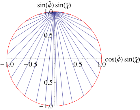
Figure 1: Lines of constant $\phi$ for a Minkowski boundary.

2 Rindler boundary

We would like to put the (2+1)-dimensional AdS metric in a form such that the conformal boundary is of the Rindler type. This can be achieved for the Rindler wedge $(x>0)$. The metric (1.3) can be written as

$$ds^{2}=\frac{1}{z^{2}}\left[dz^{2}-a^{2}x^{2}\left(1+\frac{z^{2}}{4x^{2}}\right)^{2}dt^{2}+\left(1-\frac{z^{2}}{4x^{2}}\right)^{2}dx^{2}\right].$$ (2.10)

This is a particular case of the Fefferman-Graham parametrization (1.9), characterized by a Rindler boundary at $z=0$ with metric $g_{\mu\nu}^{(0)}dx^{\mu}dx^{\nu}=-a^{2}x^{2}dt^{2}+dx^{2}$ . The coordinate transformation that achieves this does not affect the time coordinate. It is given by

$$r(z,x) = a\left(\frac{x}{z}+\frac{z}{4x}\right)$$ (2.11)

$$\phi(z,x) = \frac{1}{a}\log\left[ax\right]-\frac{8}{a(4+z^{2}/x^{2})}.$$ (2.12)

Notice that the transformation maps the whole region near negative infinity for $\phi$ to the neighborhood of zero for $x$, with $x>0$.

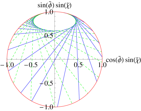
Figure 2: Lines of constant $x$ for a Rindler boundary with $a=0.5$.

A crucial property of the transformation (2.11), (2.12) is that, for fixed $x$, the function $r(z,x)$ has a minimal value at the point where $\partial r(z,x)/\partial z=0$. This relation generates the line

$$z_{t}(x)=2x,$$ (2.13)

on which

$$r_{t}(x)=a.$$ (2.14)

The corresponding values of $\phi$ are

$$\phi_{t}(x)\equiv\phi(z_{t}(x),x)=(\log[ax]-1)/a.$$ (2.15)

We have seen that $r(z,x)$ has a constant minimal value. As a result the slice $t=0$ is not fully covered by the Fefferman-Graham system of coordinates. We demonstrate this fact in fig. 2, in which we depict the form of the lines with constant $x$ and $0\leq z\leq z_{t}(x)$ for $a=0.5$. They are the solid line segments that start at the boundary and finish at some point in the interior of AdS space. The values of $x$ for each line increase as the starting point moves counterclockwise around the bounding circle. The lines with $x\to 0$ start on the left of the point ${\tilde{\phi}}={\tilde{\chi}}=\pi/2$ and infinitesimally close to it. The lines with $x\to\infty$ start on the right of this point and infinitesimally close to it. From eq. (2.12) we obtain $\phi(0,x)=(\log[ax]-2)/a$. On the boundary, the limits $x\to 0$ and $x\to\infty$ correspond to $\phi\to-\infty$ and $\phi\to\infty$, respectively. The identification of the latter two results in the identification of the first two limits as well.

The extensions of the lines when $z$ is allowed to take values $z_{t}(x)\leq z<\infty$ for given $x$ cover the AdS space for a second time, leaving the same empty region. We demostrate this feature in fig. 2. Each solid line segment (corresponding to $0\leq z\leq z_{t}(x))$ has a dashed extension (corresponding to $z_{t}(x)\leq z<\infty$) that ends on the boundary. In this way, the system of coordinates covers the AdS space twice, leaving an empty region whose boundary corresponds to $r_{t}(x)=a$. The line on which the Fefferman-Graham system of coordinates turns around and covers the AdS space for a second time is determined by $\partial r(z,x)/\partial x=0$. This relation gives again eq. (2.13), which resulted from $\partial r(z,x)/\partial z=0$. This coincidence is particular to the Rindler case. In the following section we shall consider the case of a de Sitter boundary, for which the various partial derivatives do not vanish along the same line.

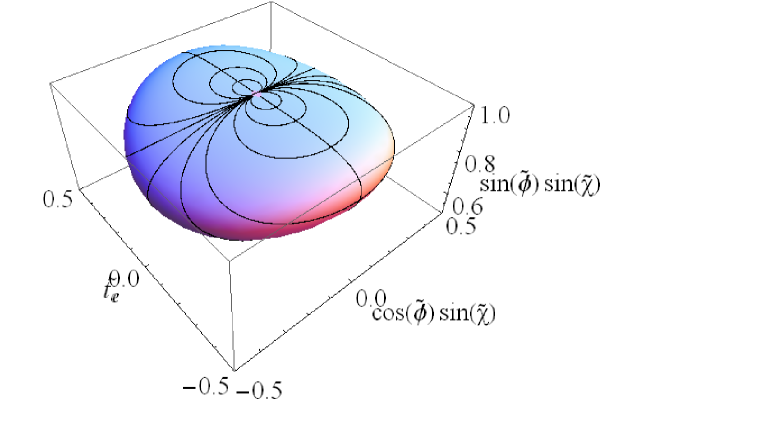
Figure 3: The region not covered by Fefferman-Graham coordinates for a Rindler boundary with $a=0.5$.

In order to examine the form of the excluded region for $t\not=0$, it is more convenient to perform a Euclidean rotation of the time coordinates appearing in the metrics (1.2) and (1.3): ${\tilde{t}}_{E}=-i\,{\tilde{t}}$, $t_{E}=-i\,t$. The global and Poincare coordinates are related through the transformation

$${\tilde{t}}_{E}(t_{E},r,\phi) = {\rm arctanh}\left[\frac{2r^{2}t_{E}}{1+r^{2}(1+\phi^{2}+t_{E}^{2})}\right]$$ (2.16)

$${\tilde{\chi}}(t_{E},r,\phi) = {\rm arctan}\sqrt{r^{2}\phi^{2}+\frac{\left[1-r^{2}(1-\phi^{2}-t_{E}^{2})\right]^{2}}{4r^{2}}}$$ (2.17)

$${\tilde{\phi}}(t_{E},r,\phi) = \arctan\left[\frac{1-r^{2}(1-\phi^{2}-t_{E}^{2})}{2r^{2}\phi}\right].$$ (2.18)

The Euclidean AdS is covered completely by both systems [5]. The Fefferman-Graham coordinates that we consider in this work result from the Poincare ones through transformations that do not involve the time coordinate. For static boundaries, the use of Euclidean time is expected to give a description of field theories on AdS equivalent to that based on Lorentzian time.

In fig. 3 we present the part of the Euclidean AdS that is not covered by Fefferman-Graham coordinates with a Rindler conformal boundary. The boundary of AdS (not shown in fig. 3) is the cylinder of radius equal to 1 that results from the continuation of the bounding circle in fig. 2 along the Euclidean time direction. In fig. 3 we depict the boundary of the excluded volume, which corresponds to the surface on which the Poincare coordinate $r$ obtains its minimal value $r=a=0.5$ . The closed circular lines on this surface have constant Poincare time $t_{E}$, while $\phi$ varies from $-\infty$ to $\infty$ along them. All these lines start and terminate at the point (${\tilde{t}}_{E}=0,{\tilde{\phi}}=\pi/2,{\tilde{\chi}}=\pi/2$) on the boundary of AdS. Each line determines the narrowest part of a throat connecting the two asymptotic regions, at $z\to 0$ and $z\to\infty$, that we discussed in the context of fig. 2 for $t_{E}=0$. In a following section we shall examine the conjecture that the length of each line is related to the entropy of the dual CFT on a (1+1)-dimensional Rindler background.

According to the AdS/CFT correspondence, the (2+1)-dimensional metric of the form (1.8), (1.9) encodes information on the dual CFT on a gravitational background given by $g_{\mu\nu}^{(0)}$. In 2+1 dimensions the Fefferman-Graham expansion terminates at the term $\sim z^{4}$. As a result we can obtain a second interpretation in terms of the dual CFT on a background with metric $g_{\mu\nu}^{(4)}$. This possibility is apparent through the simple coordinate change $z=1/z^{\prime}$. The limit $z^{\prime}\to 0$ is equivalent to the limit $z\to\infty$ that leads back to the AdS boundary, as we have seen in the example of the Rindler boundary. The Rindler case is particularly simple because the background $g_{\mu\nu}^{(4)}$ is again of the Rindler type, as can be verified through the coordinate change $x=1/(4x^{\prime})$. We can view the (part of the) AdS space covered by the Fefferman-Graham coordinates with $0\leq x<\infty$ and $0\leq z\leq z_{t}(x)$ as providing a holographic description of the dual CFT on the Rindler background at $z=0$. The second copy of (part of) the AdS space covered by $0\leq x<\infty$ and $z_{t}(x)\leq z\leq\infty$ (where the last equality corresponds to the point on the AdS boundary obtained for $z\to\infty$) describes the dual CFT on a Rindler background at $z^{\prime}=0$. In the holographic description of both dual theories, part of the AdS space is not covered by the Fefferman-Graham system of coordinates.

3 Static de Sitter boundary

We now turn to the case of a de Sitter boundary in static coordinates. The metric (1.3) can be put in the form

$$ds^{2}=\frac{1}{z^{2}}\Bigg{[}dz^{2} - (1-H^{2}\rho^{2})\left(1+\frac{1}{4}\left[\frac{H^{2}}{1-H^{2}\rho^{2}}-H^{2}\right]z^{2}\right)^{2}dt^{2}\Biggr{.}$$

. $$+ \left(1-\frac{1}{4}\left[\frac{H^{2}}{1-H^{2}\rho^{2}}+H^{2}\right]z^{2}\right)^{2}\frac{d\rho^{2}}{1-H^{2}\rho^{2}}\Biggr{]},$$ (3.19)

with a de Sitter boundary at $z=0$ with metric $g_{\mu\nu}^{(0)}dx^{\mu}dx^{\nu}=-(1-H^{2}\rho^{2})dt^{2}+d\rho^{2}/(1-H^{2}\rho^{2})$. We consider the causally connected region $-1/H<\rho<1/H$. The transformation between Poincare and Fefferman-Graham coordinates does not affect the time coordinate. It is given by

$$r(z,\rho) = \frac{\sqrt{1-H^{2}\rho^{2}}}{z}+\frac{H^{4}\rho^{2}}{4\sqrt{1-H^{2}\rho^{2}}}z$$ (3.20)

$$\phi(z,\rho) = \frac{1}{2H}\log\left[\frac{1+H\rho}{1-H\rho}\right]-\frac{H^{2}\rho z^{2}}{2(1-H^{2}\rho^{2}+H^{4}\rho^{2}z^{2}/4)}.$$ (3.21)

It is noteworthy that the transformation maps the region near $-\infty$ for $\phi$ to the vicinity of $-1/H$ for $\rho$, and the region near $\infty$ for $\phi$ to the vicinity of $1/H$ for $\rho$. The identification of the limits $\phi\to\pm\infty$ results in the identification of the limits $\rho\to\pm 1/H$ as well.

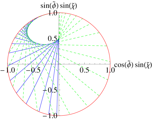
Figure 4: Lines of constant $\rho<0$ for a static de Sitter boundary with $H=0.8$.

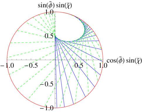
Figure 5: Lines of constant $\rho>0$ for a static de Sitter boundary with $H=0.8$.

The way in which the AdS space is covered by the Fefferman-Graham coordinates for a de Sitter boundary is more complicated that in the Rindler case. We concentrate on the $t={\tilde{t}}=0$ slice. In figs. 4, 5 we depict the form of the lines with constant positive or negative $\rho$, respectively, and $0\leq z<\infty$ for $H=0.8$. In fig. 4 the values of $\rho$ for each line increase as the starting point moves counterclockwise around the bounding circle. The solid part of each line starts from the AdS boundary, with the initial point corresponding to $z=0$. The dashed part is obtained for large values of $z$, with the boundary being approached again for $z\to\infty$. The lines with $\rho\to-1/H$ start on the left of the point ${\tilde{\phi}}={\tilde{\chi}}=\pi/2$ and infinitesimally close to it. The starting points (corresponding to $z=0$) cover half of the AdS boundary for $\rho$ taking values $-1/H\leq\rho\leq 0$. On the other hand, the endpoints (obtained for $z\to\infty$) cover the whole AdS boundary.

For the transition from the solid to the dashed part of each line we selected the point at which the system of coordinates starts covering (part of) the AdS space for a second time. This point is given by the solution of $\partial r(z,\rho)/\partial\rho=0$, which is

$$z_{t}(\rho)=\frac{2}{H}\sqrt{\frac{1-H^{2}\rho^{2}}{2-H^{2}\rho^{2}}}.$$ (3.22)

It corresponds to

$$r_{t}(\rho)\equiv r(z_{t}(\rho),\rho) = \frac{H}{\sqrt{2-H^{2}\rho^{2}}},$$ (3.23)

$$\phi_{t}(\rho) = \frac{1}{2H}\log\left[\frac{1+H\rho}{1-H\rho}\right]-\rho.$$ (3.24)

Notice that the minimal value of $r(z,\rho)$ as a function of $z$ for given $\rho$ is obtained for $\partial r(z,\rho)/\partial z=0$. This gives

$$z_{m}(\rho)=2\sqrt{\frac{1-H^{2}\rho^{2}}{H^{4}\rho^{2}}},$$ (3.25)

which satisfies $z_{m}(\rho)\geq z_{t}(\rho)$ for all $\rho$ and $z_{m}(\rho)/z_{t}(\rho)\to 1$ for $\rho\to\pm 1$.

The most interesting feature of fig. 4 is that part of the AdS slice is not covered by the coordinates. The boundary of the excluded part is not determined in general by a constant value of the Poincare coordinate $r$, as in the Rindler case. Only near the point ${\tilde{\phi}}={\tilde{\chi}}=\pi/2$ (top of the diagram), where $\rho\simeq-1/H$, the boundary of the excluded part coincides with the line of constant Poincare coordinate $r=r_{t}(|\rho|\simeq 1)\simeq H$. This means that this region maps the vicinity of one of the horizons of the (1+1)-dimensional de Sitter geometry.

In fig. 5 we depict the lines corresponding to $0\leq\rho\leq 1/H$. The solid parts of these lines start from points on the AdS boundary obtained for $z=0$. The starting points cover the second half of the AdS boundary. On the other hand, the endpoints of the lines at the end of the dashed segments, obtained for $z\to\infty$, cover the full AdS boundary. There is a part of the AdS slice that is not covered by the coordinates. Near the top of the diagram, the boundary of the excluded part coincides with the line of constant $r=r_{m}(\rho\simeq 1)\simeq H$. This region maps the vicinity of the second horizon of the (1+1)-dimensional geometry.

Similarly to the Rindler case, we view the (part of the) AdS space covered by the Fefferman-Graham coordinates with $-1\leq\rho\leq 1$ and $0\leq z\leq z_{t}(\rho)$ as providing a holographic description of the dual CFT on the static de Sitter background at $z=0$. The second copy of (part of) the AdS space covered by $-1\leq\rho\leq 1$ and $z_{t}(\rho)\leq\rho\leq\infty$ (where the last equality corresponds to the point on the AdS boundary obtained for $z\to\infty$) describes the dual CFT on a different background at $z^{\prime}=1/z=0$. Contrary to the Rindler case, this second background does not have an obvious physical interpretation. For this reason we concentrate on the dual theory at $z=0$. On the gravity side, we consider only the part of AdS covered by the solid lines in figs. 4, 5.

The extension of this picture to the full AdS geometry is too complicated to be represented pictorially. However, for static boundary metrics, such as the ones we are considering, the determination of thermodynamic properties of the dual CFT can be performed at any time. We shall confirm this fact for the Rindler entropy in the next section. On the other hand, for the de Sitter entropy we shall consider only the slice $t={\tilde{t}}=0$.

4 Horizons and entropy

The proposal of ref. [9] is that the entropy associated with the dual theory on a nontrivial background is related to the part of the AdS space not covered by the Fefferman-Graham system of coordinates. More specifically, the entropy at a given time is assumed to be proportional to the length $A$ of the line defining the boundary of the part of AdS not covered by the coordinates. The exact relation between the entropy $S$ and the length $A$ is

$$S=\frac{1}{4G_{3}}A,$$ (4.26)

with $G_{3}$ Newton’s constant of the (2+1)-dimensional theory. In the following we review how this expression reproduces the Rindler and de Sitter entropies. The detailed calculation has been presented in ref. [9], but several related issues are clarified through inspection of figs. 2-5.

For a Rindler boundary at $z=0$, the part of AdS space not covered by the coordinates (2.10) is delimited by the line of constant $r$ given by eq. (2.14) . For $t=0$ the omitted region is depicted in fig. 2. The corresponding values of $z$ and $\phi$ are given by eqs. (2.13, (2.15), respectively. The entropy can be expressed as a line integral, with various forms depending on the integration variable:

$$S=\frac{1}{4G_{3}}\int_{-\infty}^{\infty}ad\phi=\frac{1}{4G_{3}}\int_{0}^{\infty}\frac{dx}{x}=\frac{1}{4G_{3}}\int_{0}^{\infty}\frac{dz}{z}.$$ (4.27)

All the above integrals are infinite. The divergences arise from the two ends of the line that approach the point ${\tilde{\phi}}={\tilde{\chi}}=\pi/2$ (top of the diagram of fig. 2). The last integral in eq. (4.27) demonstrates that the divergence is related to the infinite volume near the boundary of AdS space. The way to handle this situation is to introduce a cutoff $\epsilon$ for the line element, with $\epsilon\ll 1$. The dominant contribution to the integral of eq. (4.27) can be written as

$$S=\frac{2}{4G_{3}}\int_{\epsilon}\frac{dz}{z},$$ (4.28)

with the factor of 2 arising from the two limits $\phi\to\pm\infty$. We have not introduced an explicit upper limit, as its exact value is irrelevant for $\epsilon\to 0$.

In order to extract the physical meaning of eq. (4.28), we must compare it with the effective Newton’s constant $G_{2}$ of the (1+1)-dimensional theory. For a theory living on the $z=0$ boundary, $G_{2}$ is given by the expression.

$$\frac{1}{G_{2}}=\frac{1}{G_{3}}\int_{\epsilon}\frac{dz}{z}.$$ (4.29)

The cutoff $\epsilon$ is again introduced in order to regulate a divergence generated by the infinite AdS volume near the boundary. We have omitted the upper limit, as the integral is dominated by the lower one for $\epsilon\to 0$. The fact that $G_{2}$ tends to zero in the same limit is consistent with the absence of dynamics for the boundary gravity in the context of AdS/CFT.

Comparison of eqs. (4.28), (4.29) indicates that we can interpret eq. (4.27) as

$$S=\frac{2}{4G_{2}}.$$ (4.30)

Repeating the calculation of ref. [12] for the two-dimensional case results in an expression for the entropy of the two-dimensional Rindler wedge that is half the value given by eq. (4.30). The discrepancy is related to the symmetry around the vertical axis of the region not covered by the Fefferman-Graham coordinates in fig. 2. The origin of this feature can be traced to the periodicity of the global coordinate ${\tilde{\phi}}$ arising from the compactness of the spatial direction on the AdS boundary. As a result, in the construction with a Rindler conformal boundary, the limits $x\to 0$ and $x\to\infty$ of the Fefferman-Graham coordinate $x$ must be identified. The two limits correspond to the two regions on either side of the point ${\tilde{\phi}}={\tilde{\chi}}=\pi/2$ in fig. 2, which are completely symmetric. The region on the left provides a holographic description of the vicinity of the Rindler horizon at $x=0$. The region on the right has an identical form, mimicking the presence of a horizon at $x\to\infty$. We are thus led to the conclusion that the construction of section 2 does not represent the conventional Rindler space. It provides a holographic description of the Rindler wedge ($0\leq x<\infty$), with an identification of the limits $x\to 0$ and $x\to\infty$.

The above considerations indicate that the entropy of the conventional Rindler space is associated only with the region near $x=0$, which provides an acceptable holographic description of the vicinity of the Rindler horizon. The defining feature is the absence of complete coverage of the $t=0$ slice of AdS space. The entropy can be identified with the length of the boundary of the excluded region. This is dominated by the part of the line near the AdS boundary, and is given by

$$S_{R}=\frac{1}{4G_{2}}.$$ (4.31)

The extension of this feature to different time slices is given in fig. 3. All slices of constant Euclidean time $t_{E}$ (closed circular lines in fig. 3) go through the point ${\tilde{\phi}}={\tilde{\chi}}=\pi/2$ on the AdS boundary. Repeating the above analysis for anyone of them will lead to eq. (4.31), as the expression for the entropy is dominated by the divergent integral near the AdS boundary.

The case of a de Sitter boundary has a more straightforward interpretation. The identification of the limits $\rho\to\pm 1/H$, imposed by the periodicity of the global coordinate ${\tilde{\phi}}$, does not alter the physical picture, because the two limits correspond to the two symmetric horizons of the (1+1)-dimensional de Sitter space. The part of the AdS space covered by the solid lines in figs. 4, 5 provides a holographic description of the causally connected region between the horizons. The horizons and their vicinity are mapped on the boundary of the region covered by the Fefferman-Graham coordinates in the neighborhood of the point ${\tilde{\phi}}={\tilde{\chi}}=\pi/2$. The sum of the lengths of the two lines delimiting this region and ending at the point ${\tilde{\phi}}={\tilde{\chi}}=\pi/2$ gives the de Sitter entropy. The entropy is given by eq. (4.28), which results in

$$S_{dS}=\frac{1}{2G_{2}}.$$ (4.32)

This is the correct expression for the entropy of two-dimensional de Sitter space [13].

Based on the above, we can conclude that, in the context of the AdS/CFT correspondence, it seems natural to attribute the entropy of the dual theory on a certain boundary metric to the presence of a part of the AdS space that is not covered by the Fefferman-Graham coordinates. These have a special status, at they are adopted to a boundary observer and provide a natural holographic interpretion of the bulk space. The clearest example of the connection between the boundary entropy and the lack of coverage of the AdS space by the coordinates involves the BTZ black hole in the bulk with a Minkowski conformal boundary [9]. The examples of a Rindler and de Sitter boundary that we discussed in detail provide additional support for this connection. The implications for a configuration with an AdS black hole in the bulk and an expanding boundary have been discussed in refs. [14, 15, 16, 9].

From the holographic perspective, the bulk space may be viewed as a represenation of the boundary CFT, with the extra dimension playing the role of the energy scale. In the examples we discussed the bulk is locally isomorphic to AdS space, while for certain boundary metrics there are bulk regions that are not covered by the coordinates. A bulk field with an arbitrary dependence on the Fefferman-Graham coordinates will not take values in these AdS regions. Our suggestion is that, since this part of the bulk is not included in the construction of the dual theory, it must be associated with the entropy of the CFT. This definition of entropy bears strong similarity to the entropy generated by quantum entanglement between classically disconnected regions of space.

For Rindler and de Sitter bounaries, a horizon of the boundary metric plays a special role. It defines a point separating two causally disconnected regions of the boundary. It also determines the beginning of the line delimiting the part of the bulk excluded by the Fefferman-Graham parametrization. We can view the horizon as the holographic image of the part of this line in the near-boundary region. The entropy is proportional either to area of the horizon, or the area of its bulk extension. The two areas have different dimensionalities. However, the proportionallity constants in the two cases (involving the effective or the bulk Newtons’s constant, respectively) compensate for this difference.

As a final comment, we point out that the holographic interpretation of entropy is not necessarily bound to the presence of a horizon. For a BTZ bulk and a Minkowski boundary, there is no horizon on the boundary. However, the connection with the entropy persists: The excluded part of the bulk lies away from the boundary and is related to the thermal entropy of the dual CFT [9].

References

- [1] J. M. Maldacena, Adv. Theor. Math. Phys. 2 (1998) 231 [Int. J. Theor. Phys. 38 (1999) 1113] [arXiv:hep-th/9711200].
-
[2]
S. S. Gubser, I. R. Klebanov and A. M. Polyakov,
Phys. Lett. B 428 (1998) 105
[arXiv:hep-th/9802109];
E. Witten, Adv. Theor. Math. Phys. 2 (1998) 253 [arXiv:hep-th/9802150]. - [3] C. Fefferman and C. Robin Graham, Conformal Invariants, in Elie Cartan et les Mathématiques d’aujourd’hui, Astérisque, 1985, page 95.
- [4] S. de Haro, S. N. Solodukhin and K. Skenderis, Commun. Math. Phys. 217 (2001) 595 [arXiv:hep-th/0002230]; Class. Quant. Grav. 19 (2002) 5849 [arXiv:hep-th/0209067].
- [5] O. Aharony, S. S. Gubser, J. M. Maldacena, H. Ooguri and Y. Oz, Phys. Rept. 323 (2000) 183 [arXiv:hep-th/9905111].
- [6] C. A. Bayona, N. R. F. Braga, Gen. Rel. Grav. 39 (2007) 1367-1379. [hep-th/0512182].
- [7] K. Skenderis and B. C. van Rees, Commun. Math. Phys. 301 (2011) 583 [arXiv:0912.2090 [hep-th]].
- [8] K. Skenderis and S. N. Solodukhin, Phys. Lett. B 472 (2000) 316 [arXiv:hep-th/9910023].
- [9] N. Tetradis, [arXiv:1106.2492 [hep-th]].
- [10] N. D. Birrell and P. C. W. Davis, Quantum fields in curved space, Cambridge Monographs on Mathematical Physics, Cambridge University Press, 1982.
- [11] L. Randall and R. Sundrum, Phys. Rev. Lett. 83 (1999) 3370 [arXiv:hep-th/9905221]; Phys. Rev. Lett. 83 (1999) 4690 [arXiv:hep-th/9906064].
- [12] R. Laflamme, Phys. Lett. B 196 (1987) 449.
- [13] S. Hawking, J. M. Maldacena and A. Strominger, JHEP 0105 (2001) 001 [arXiv:hep-th/0002145].
- [14] P. S. Apostolopoulos, G. Siopsis and N. Tetradis, Phys. Rev. Lett. 102 (2009) 151301 [arXiv:0809.3505 [hep-th]].
- [15] N. Tetradis, JHEP 1003 (2010) 040 [arXiv:0905.2763 [hep-th]]; J. Phys. Conf. Ser. 283 (2011) 012038.
- [16] N. Lamprou, S. Nonis and N. Tetradis, arXiv:1106.1533 [gr-qc].