Feature-Based Matrix Factorization

Abstract

Recommender system has been more and more popular and widely used in many applications recently. The increasing information available, not only in quantities but also in types, leads to a big challenge for recommender system that how to leverage these rich information to get a better performance. Most traditional approaches try to design a specific model for each scenario, which demands great efforts in developing and modifying models. In this technical report, we describe our implementation of feature-based matrix factorization. This model is an abstract of many variants of matrix factorization models, and new types of information can be utilized by simply defining new features, without modifying any lines of code. Using the toolkit, we built the best single model reported on track 1 of KDDCup’11.

1 Introduction

Recommender systems that recommends items based on users interest has become more and more popular among many web sites. Collaborative Filtering(CF) techniques that behind the recommender system have been developed for many years and keep to be a hot area in both academic and industry aspects. Currently CF problems face two kinds of major challenges: how to handle large-scale dataset and how to leverage the rich information of data collected.

Traditional approaches to solve these problems is to design specific models for each problem, i.e writing code for each model, which demands great efforts in engineering. Matrix factorization(MF) technique is one of the most popular method of CF model, and extensive study has been made in different variants of matrix factorization model, such as [3][4] and [5]. However, we find that the majority of matrix factorization models share common patterns, which motivates us to put them together into one. We call this model feature-based matrix factorization. Moreover, we write a toolkit for solving the general feature-based matrix factorization problem, saving the efforts of engineering for detailed kinds of model. Using the toolkit, we get the best single model on track 1 of KDDCup’11[2].

This article serves as a technical report for our toolkit of feature-based matrix factorization. We try to elaborate three problems in this report, i.e, what the model is, how can we use such kind of model, and additional discussion of issues in engineering and efficient computation.

2 What is feature based MF

In this section, we will describe the model of feature based matrix factorization, starting from the example of linear regression, and then going to the full definition of our model.

2.1 Start from linear regression

Let’s start from the basic collaborative filtering models. The very baseline of collaborative filtering model may be the baseline models just considering the mean effect of user and item. See the following two models.

$$\hat{r}_{ui}=\mu+b_{u}$$ (1)

$$\hat{r}_{ui}=\mu+b_{u}+b_{i}$$ (2)

Here $\mu$ is a constant indicating the global mean value of rating. Equation 1 describe a model considering users’ mean effect while Equation 2 denotes items’ mean effect. A more complex model considering the neighborhood information[3] is as follows

$$\hat{r}_{ui}=\mu+b_{i}+b_{u}+|R(u)|^{-\frac{1}{2}}\sum_{j\in R(u)}s_{ij}(r_{uj}-\bar{b}_{u})$$ (3)

Here $R(u)$ is the set of items user $u$ rate, $\bar{b}_{u}$ is a user average rating pre-calculated. $s_{ij}$ means the similarity parameter from $i$ to $j$. $s_{ij}$ is a parameter that we train from data instead of direct calculation using memory based methods. Note $\bar{b}_{u}$ is different from $b_{u}$ since it’s pre-calculated. This is a neighborhood model that takes the neighborhood effect of items into consideration.

Assuming we want to implement all three models, it seems to be wasting to write code for each of the model. If we compare those models, it is obvious that all the three models are special cases of linear regression problem described by Equation 4

$$y=\sum_{i}w_{i}x_{i}$$ (4)

Suppose we have $n$ users, $m$ items, and $h$ total number of possible $s_{ij}$ in equation 3. We can define the feature vector $x=[x_{0},x_{1},\cdots,x_{n+m+h}]$ for user item pair $<u,i>$ as follows

$$x_{k}=\left\{\begin{array}[]{ll}Indicator(u==k)&k<n\\ Indicator(i==k-n)&n\leq k<n+m\\ 0&k\geq m+n,j\notin R(u),\mbox{$s_{ij}$ means $w_{k}$}\\ |R(u)|^{-\frac{1}{2}}(r_{uj}-\bar{b}_{u})&k\geq m+n,j\in R(u),\mbox{$s_{ij}$ means $w_{k}$}\\ \end{array}\right.$$ (5)

The corresponding layout for weight $w$ shown in equation 6. Note that choice of pairs $s_{ij}$ can be flexible. We can choose only possible neighbors instead of enumerating all the pairs.

$$w=[b_{u}(0),b_{u}(1),\cdots,b_{u}(n),b_{i}(1),\cdots b_{i}(m)\cdots s_{ij}\cdots]$$ (6)

In other words, equation 3 can be reformed as the following form

$$\hat{r}_{ui}=\mu+b_{i}1+b_{u}1+\sum_{j\in R(u)}s_{ij}\left[|R(u)|^{-\frac{1}{2}}(r_{uj}-\bar{b}_{u})\right]$$ (7)

where $b_{i}$, $b_{u}$, $s_{ij}$ corresponds to weight of linear regression, and the coefficients on the right of the weight are the input features. In summary, under this framework, the only thing that we need to do is to layout the parameters into a feature vector. In our case, we arrange first $n$ features to $b_{u}$ then $b_{i}$ and $s_{ij}$, then transform the input data into the format of linear regression input. Finally we use a linear regression solver to work the problem out.

2.2 Feature based matrix factorization

The previous section shows that some baseline CF algorithms are linear regression problem. In this section, we will discuss feature-based generalization for matrix factorization. A basic matrix factorization model is stated in Equation 8:

$$\hat{r}_{ui}=\mu+b_{u}+b_{i}+p^{T}_{u}q_{i}$$ (8)

The bias terms have the same meaning as previous section. We also get two factor term $p_{u}$ and $q_{i}$. $p_{u}$ models the latent peference of user $u$. $q_{i}$ models the latent property of item $i$.

Inspired by the idea of previous section, we can get a direct generalization for matrix factorization version.

$$\hat{r}_{ui}=\mu+\sum_{j}w_{j}x_{j}+b_{u}+b_{i}+p^{T}_{u}q_{i}$$ (9)

Equation 9 adds a linear regression term to the traditional matrix factorization model. This allows us to add more bias information, such as neighborhood information and time bias information, etc. However, we may also need a more flexible factor part. For example, we may want a time dependent user factor $p_{u}(t)$ or hierarchical dependent item factor $q_{i}(h)$. As we can find from previous section, a direct way to include such flexibility is to use features in factor as well. So we adjust our feature based matrix factorization as follows

$$y=\mu+\left(\sum_{j}b^{(g)}_{j}\gamma_{j}+\sum_{j}b^{(u)}_{j}\alpha_{j}+\sum_{j}b^{(i)}_{j}\beta_{j}\right)+\left(\sum_{j}p_{j}\alpha_{j}\right)^{T}\left(\sum_{j}q_{j}\beta_{j}\right)$$ (10)

The input consists of three kinds of features $<\alpha,\beta,\gamma>$, we call $\alpha$ user feature, $\beta$ item feature and $\gamma$ global feature. The first part of Equation 10. The name of these features explains their meanings. $\alpha$ describes the user aspects, $\beta$ describes the item aspects, while $\gamma$ describes some global bias effect. Figure 1 shows the idea of the procedure.

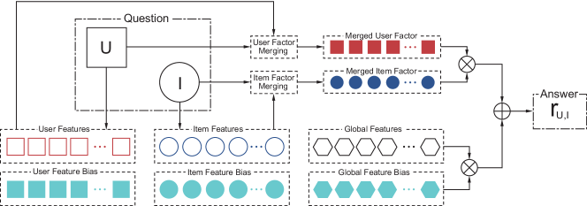
Figure 1: Feature-based matrix factorization

We can find basic matrix factorization is a special case of Equation 10. For predicting user item pair $<u,i>$, define

$$\gamma=\emptyset,\ \alpha_{k}=\left\{\begin{array}[]{ll}1&k=u\\ 0&k\neq u\\ \end{array}\right.,\ \beta_{k}=\left\{\begin{array}[]{ll}1&k=i\\ 0&k\neq i\\ \end{array}\right.$$ (11)

We are not limited to the simple matrix factorization. It enables us to incorporate the neighborhood information to $\gamma$, and time dependent user factor by modifying $\alpha$. Section 3 will present a detailed description of this.

2.3 Active function and loss function

There, you need to choose an active function $f(\cdot)$ to the output of the feature based matrix factorization. Similarly, you can also try various of loss functions for loss estimation. The final version of the model is

$$\hat{r}=f(y)$$ (12)

$$Loss=L(\hat{r},r)+regularization$$ (13)

Common choice of active functions and loss are listed as follows:

• identity function, L2 loss, original matrix factorization.

  $$\hat{r}=f(y)=y$$ (14)

  $$Loss=(r-\hat{r})^{2}+regularization$$ (15)

• sigmoid function, log likelihood, logistic regression version of matrix factorization.

  $$\hat{r}=f(y)=\frac{1}{1+e^{-y}}$$ (16)

  $$Loss=r\ln\hat{r}+(1-r)\ln(1-\hat{r})+regularization$$ (17)

• identity function, smoothed hinge loss[7], maximum margin matrix factorization[8][7]. Binary classification problem, $r\in\{0,1\}$

  $$Loss=h\left((2r-1)y\right)+regularization$$ (18)

  $$h(z)=\left\{\begin{array}[]{ll}\frac{1}{2}-z&z\leq 0\\ \frac{1}{2}(1-z)^{2}&0<z<1\\ 0&z\geq 1\\ \end{array}\right.$$ (19)

2.4 Model Learning

To update the model, we use the following update rule

$$p_{i} =p_{i}+\eta\left(\hat{e}\alpha_{i}\left(\sum_{j}q_{j}\beta_{j}\right)-\lambda_{1}p_{i}\right)$$ (20)

$$q_{i} =q_{i}+\eta\left(\hat{e}\beta_{i}\left(\sum_{j}p_{j}\alpha_{j}\right)-\lambda_{2}q_{i}\right)$$ (21)

$$b^{(g)}_{i} =b^{(g)}_{i}+\eta\left(\hat{e}\gamma_{i}-\lambda_{3}b^{(g)}_{i}\right)$$ (22)

$$b^{(u)}_{i} =b^{(u)}_{i}+\eta\left(\hat{e}\alpha_{i}-\lambda_{4}b^{(u)}_{i}\right)$$ (23)

$$b^{(i)}_{i} =b^{(i)}_{i}+\eta\left(\hat{e}\beta_{i}-\lambda_{5}b^{(i)}_{i}\right)$$ (24)

Here $\hat{e}=r-\hat{r}$ the difference between true rate and predicted rate. This rule is valid for both logistic likelihood loss and L2 loss. For other loss, we shall modify $\hat{e}$ to be corresponding gradient. $\eta$ is the learning rate and the $\lambda$s are regularization parameters that defines the strength of regularization.

3 What information can be included

In this section, we will present some examples to illustrate the usage of our feature-based matrix factorization model.

3.1 Basic matrix factorization

Basic matrix factorization model is defined by following equation

$$y=\mu+b_{u}+b_{i}+p^{T}_{u}q_{i}$$ (25)

And the corresponding feature representation is

$$\gamma=\emptyset,\ \alpha_{k}=\left\{\begin{array}[]{ll}1&k=u\\ 0&k\neq u\\ \end{array}\right.,\ \beta_{k}=\left\{\begin{array}[]{ll}1&k=i\\ 0&k\neq i\\ \end{array}\right.$$ (26)

3.2 Pairwise rank model

For the ranking model, we are interested in the order of two items $i,j$ given a user $u$. A pairwise ranking model is described as follows

$$P(r_{ui}>r_{uj})=sigmoid\left(\mu+b_{i}-b_{j}+p^{T}_{u}(q_{i}-q_{j})\right)$$ (27)

The corresponding features representation are like this

$$\gamma=\emptyset,\ \alpha_{k}=\left\{\begin{array}[]{ll}1&k=u\\ 0&k\neq u\\ \end{array}\right.,\ \beta_{k}=\left\{\begin{array}[]{ll}1&k=i\\ -1&k=j\\ 0&k\neq i,k\neq j\\ \end{array}\right.$$ (28)

by using sigmoid and log-likelihood as loss function. Note that the feature representation gives one extra $b_{u}$ which is not desirable. We can removed it by give high regularization to $b_{u}$ that penalize it to $0$.

3.3 Temporal Information

A model that include temporal information[4] can be described as follows

$$y=\mu+b_{u}(t)+b_{i}(t)+b_{u}+b_{i}+\left(p_{u}+p_{u}(t)\right)^{T}q_{i}$$ (29)

We can include $b_{i}(t)$ using global feature, and $b_{u}(t)$, $p_{u}(t)$ using user feature. For example, we can define a time interpolation model as follows

$$y=\mu+b_{i}+b^{s}_{u}\frac{e-t}{e-s}+b^{e}_{u}\frac{t-s}{e-s}+\left(p^{s}_{u}\frac{e-t}{e-s}+p^{e}_{u}\frac{t-s}{e-s}\right)^{T}q_{i}$$ (30)

Here $e$ and $s$ mean start and end of the time of all the ratings. A rating that’s rated later will be affected more by $p^{e}$ and $b^{e}$ and earlier ratings will be more affected by $p^{s}$ and $b^{s}$. For this model, we can define

$$\gamma=\emptyset,\ \alpha_{k}=\left\{\begin{array}[]{ll}\frac{e-t}{e-s}&k=u\\ \frac{t-s}{e-s}&k=u+n\\ 0&\mbox{otherwise}\\ \end{array}\right.,\ \beta_{k}=\left\{\begin{array}[]{ll}1&k=i\\ 0&k\neq i\\ \end{array}\right.$$ (31)

Note we first arrange the $p^{s}$ in the first $n$ features then $p^{e}$ in next $n$ features.

3.4 Neighborhood information

A model that include neighborhood information[3] can be described as below:

$$y=\mu+\sum_{j\in R(u)}s_{ij}\left[|R(u)|^{-\frac{1}{2}}(r_{uj}-\bar{b}_{u})\right]+b_{u}+b_{i}+p^{T}_{u}q_{i}$$ (32)

We only need to implement neighborhood information to global features as described by Section 2.1.

3.5 Hierarchical information

In Yahoo! Music Dataset[2], some tracks belongs to same artist. We can include such hierarchical information by adding it to item feature. The model is described as follows

$$y=\mu+b_{u}+b_{t}+b_{a}+p_{u}^{T}(q_{t}+q_{a})$$ (33)

Here $t$ means track and $a$ denotes corresponding artist. This model can be formalized as feature-based matrix factorization by redefining item feature.

4 Efficient training for SVD++

Feature-based matrix factorization can naturally incorporate implicit and explicit information. We can simply add these information to user feature $\alpha$. The model configuration is shown as follows:

$$y=bias+\left(\sum_{j}\xi_{j}p_{j}+\sum_{j}\alpha_{j}d_{j}\right)^{T}\left(\sum_{j}\beta_{j}q_{j}\right)$$ (34)

Here we omit the detail of bias term. The implicit and explicit feedback information is given by $\sum_{j}\alpha_{j}d_{j}$, where $\alpha$ is the feature vector of feedback information, $\alpha_{j}=\frac{1}{\sqrt{|R(u)|}}$ for implicit feedback, and $\alpha_{j}=\frac{r_{u,j}-b_{u}}{\sqrt{|R(u)|}}$ for explicit feedback. $d_{j}$ is the parameter of implicit and explicit feedback factor. We explicitly state out the implicit and explicit information in Equation 34.

Although Equation 34 shows that we can easily incorporate implicit and explicit information into the model, it’s actually very costly to run the stochastic gradient training, since the update cost is linear to the size of nonzero entries of $\alpha$, and $\alpha$ can be very large if a user has rated many items. This will greatly slow down the training speed. We need to use an optimized method to do training. To show the idea of the optimized method, let’s first define a derived user implicit and explicit factor $p^{im}$ as follows:

$$p^{im}=\sum_{j}\alpha_{j}d_{j}$$ (35)

The update of $d_{j}$ after one step is given by the following equation

$$\Delta d_{j}=\eta\hat{e}\alpha_{j}\left(\sum_{j}\beta_{j}q_{j}\right)$$ (36)

The resulted difference in $p^{im}$ is given by

$$\Delta p^{im}=\eta\hat{e}\left(\sum_{j}\alpha^{2}_{j}\right)\left(\sum_{j}\beta_{j}q_{j}\right)$$ (37)

Given a group of samples with the same user, we need to do gradient descent on each of the training sample. The simplest way is to do the following steps for each sample: (1) calculate $p^{im}$ to get prediction (2) update all $d_{j}$ associates with implicit and explicit feedback. Every time $p^{im}$ has to be recalculated using updated $d_{j}$ in this way. However, we can find that to get new $p^{im}$, we don’t need to update each $d_{j}$. Instead, we only need to update $p^{im}$ using Equation 37. What’s more, we can find there is a relation between $\Delta p^{im}$ and $\Delta d_{j}$ as follows:

$$\Delta d_{j}=\frac{\alpha_{j}}{\sum_{k}\alpha_{k}^{2}}\Delta p^{im}$$ (38)

We shall emphasize that Equation 38 is true even for multiple updates, given the condition that the user is same in all the samples. We shall mention that the above analysis doesn’t consider the regularization term. If L2 regularization of $d_{j}$ is used during the update as follows:

$$\Delta d_{j}=\eta\left(\hat{e}\alpha_{j}\left(\sum_{j}\beta_{j}q_{j}\right)-\lambda d_{j}\right)$$ (39)

The corresponding changes in $p^{im}$ also looks very similar

$$\Delta p^{im}=\eta\left(\hat{e}\left(\sum_{j}\alpha^{2}_{j}\right)\left(\sum_{j}\beta_{j}q_{j}\right)-\lambda p^{im}\right)$$ (40)

However, the relation in Equation 38 no longer holds strictly. But we can still use the relation since it approximately holds when regularization term is small. Using the results we obtained, we can develop a fast algorithm for feature-based matrix factorization with implicit and explicit feedback information. The algorithm is shown in Algorithm 1.

Algorithm 1 Efficient Training for Implicit and Explicit Feedback

  for all user $u$ do

     $p^{im}\leftarrow\sum_{j}\alpha_{j}d_{j}$ {calculating implicit feedback}

     $p^{old}\leftarrow p^{im}$

     for all training samples of user $u$ do

        update other parameters, using $p^{im}$ to replace $\sum_{j}\alpha_{j}d_{j}$

        update $p^{im}$ directly , do not update $d_{j}$.

     end for

     for all $i,\alpha_{i}\neq 0$ do

        $d_{i}\leftarrow d_{i}+\frac{\alpha_{i}}{\sum_{k}\alpha_{k}^{2}}(p^{im}-p^{old})$ {add all the changes back to $d$}

     end for

  end for

We find that the basic idea is to group the data of the same user together, for the same user shares the same implicit and explicit feedback information. Algorithm 1 allows us to calculate implicit feedback factor only once for a user, greatly saving the computation time.

5 How large-scale data is handled

Recommender system confronts the problem of large-scale data in practice. This is a must when dealing with real problems. For example Yahoo! Music Dataset[2] consists of more than 200M ratings. A toolkit that’s robust to input data size is desirable for real applications.

5.1 Input data buffering

The input training data is extremely large in real application, we don’t try to load all the training data into memory. Instead, we buffer all the training data through binary format into the hard-disk. We use stochastic gradient descend to train our model, that is we only need to linearly iterate over the data if we shuffle our data before buffering.

Therefore, our solution requires the input feature to be previously shuffled, then a buffering program will create a binary buffer from the input feature. The training procedure reads the data from hard-disk and uses stochastic gradient descend to train the model. This buffering approach makes the memory cost invariant to the input data size, and allows us to train models over large-scale of input data so long as the parameters fit into memory.

5.2 Execution pipeline

Although input data buffering can solve the problem of large-scale data, it still suffers from the cost of reading the data from hard-disk. To minimize the cost of I/O, we use a pre-fetching strategy. We create a independent thread to fetch the buffer data into a memory queue, then the training program reads the data from memory queue and do training. The procedure is shown in Figure 2

Figure 2: Execution pipeline

This pipeline style of execution removes the burden of I/O from the training thread. So long as I/O speed is similar or faster to training speed, the cost of I/O is negligible, and our our experience on KDDCup’11 proves the success of this strategy. With input buffering and pipeline execution, we can train a model with test RMSE=22.16 for track1 in KDDCup’11 using less than 2G of memory, without significantly increasing of training time.

6 Related work and discussion

The most related work of feature based matrix factorization is Factorization Machine [6]. The reader can refer to libFM for a toolkit for factorization machine. Strictly speaking, our toolkit implement a restricted case of factorization machine and is more useful in some aspects. We can support global feature that doesn’t need to be take into factorization part, which is important for bias features such as user day bias, neighborhood based features, etc. The divide of features also gives hints for model design. For global features, we shall consider what aspect may influence the overall rating. For user and item features, we shall consider how to describe the user preference and item property better. Our model is also related to [1] and [9], the difference is that in feature-based matrix factorization, the user/item feature can associate with temporal information and other context information to better describe the preference or property in current context. Our current model also has shortcomings. The model doesn’t support multiple distinct factorizations at present. For example, sometimes we may want to introduce user vs time tensor factorization together with user vs item factorization. We will try our best to overcome these drawbacks in the future works.

References

- [1] Deepak Agarwal and Bee-Chung Chen. Regression-based latent factor models. In Proceedings of the 15th ACM SIGKDD international conference on Knowledge discovery and data mining, KDD ’09, pages 19–28, New York, NY, USA, 2009. ACM.
- [2] Gideon Dror, Noam Koenigstein, Yehuda Koren, and Markus Weimer. The Yahoo! Music dataset and KDD-Cup’11. In KDD-Cup Workshop, 2011.
- [3] Yehuda Koren. Factorization meets the neighborhood: a multifaceted collaborative filtering model. In Proceeding of the 14th ACM SIGKDD international conference on Knowledge discovery and data mining, KDD ’08, pages 426–434, New York, NY, USA, 2008. ACM.
- [4] Yehuda Koren. Collaborative filtering with temporal dynamics. In Proceedings of the 15th ACM SIGKDD international conference on Knowledge discovery and data mining, KDD ’09, pages 447–456, New York, NY, USA, 2009. ACM.
- [5] A. Paterek. Improving regularized singular value decomposition for collaborative filtering. In Proceedings of KDD Cup and Workshop, volume 2007, 2007.
- [6] Steffen Rendle. Factorization machines. In Proceedings of the 10th IEEE International Conference on Data Mining. IEEE Computer Society, 2010.
- [7] Jasson D. M. Rennie and Nathan Srebro. Fast maximum margin matrix factorization for collaborative prediction. In Proceedings of the 22nd international conference on Machine learning, ICML ’05, pages 713–719, New York, NY, USA, 2005. ACM.
- [8] Nathan Srebro, Jason D. M. Rennie, and Tommi S. Jaakola. Maximum-Margin Matrix Factorization. In Advances in Neural Information Processing Systems 17, volume 17, pages 1329–1336, 2005.
- [9] David H. Stern, Ralf Herbrich, and Thore Graepel. Matchbox: large scale online bayesian recommendations. In Proceedings of the 18th international conference on World wide web, WWW ’09, pages 111–120, New York, NY, USA, 2009. ACM.