Reducing combinatorial uncertainties:
A new technique based on $M_{T2}$ variables

Abstract

We propose a new method to resolve combinatorial ambiguities in hadron collider events involving two invisible particles in the final state. This method is based on the kinematic variable $M_{T2}$ and on the $M_{T2}$-assisted-on-shell reconstruction of invisible momenta, that are reformulated as ‘test’ variables $T_{i}$ of the correct combination against the incorrect ones. We show how the efficiency of the single $T_{i}$ in providing the correct answer can be systematically improved by combining the different $T_{i}$ and/or by introducing cuts on suitable, combination-insensitive kinematic variables. We illustrate our whole approach in the specific example of top anti-top production, followed by a leptonic decay of the $W$ on both sides. However, by construction, our method is also directly applicable to many topologies of interest for new physics, in particular events producing a pair of undetected particles, that are potential dark-matter candidates. We finally emphasize that our method is apt to several generalizations, that we outline in the last sections of the paper.

1 Introduction

Many models providing WIMP dark-matter candidates predict events at the Large Hadron Collider (LHC), characterized by a pair of invisible particles in the final state. This very same topology is also available in the Standard Model (SM), e.g. in dileptonic decays of a top-quark pair: $t\bar{t}\to b\ell^{+}\nu\bar{b}\ell^{-}\bar{\nu}$. Several kinematic methods have been proposed to determine the particle masses in such missing energy events Barr:2010zj . On the other hand, to access information beyond the mass, e.g. the spin and/or chirality of parent particles, it is very often highly desirable, sometimes necessary, to reconstruct the parent particles’ full momenta event by event. Such reconstruction generically suffers from the combinatorial ambiguity of correctly assigning visible particles to the given event topology. For instance, there are two possibilities to pair the two $b$-jets and the two charged leptons in the dileptonic decay of a top quark pair, and three possibilities to group the jets into two dijets in the gluino pair decay $\tilde{g}\tilde{g}\rightarrow jj\tilde{\chi}_{1}^{0}jj\tilde{\chi}_{1}^{0}$ in supersymmetric models, $\tilde{\chi}_{1}^{0}$ denoting the LSP neutralino. Not to mention that the possible combinations proliferate when the event involves multi-step cascade decays and one wishes to identify the order of visible particles in each decay chain, besides the assignment to the correct decay chain. For instance, in the event $\tilde{\chi}_{2}^{0}\tilde{\chi}_{2}^{0}\rightarrow\tilde{\ell}^{\pm}\ell^{\mp}\tilde{\ell}^{\pm}\ell^{\mp}\rightarrow\ell^{+}\ell^{-}\tilde{\chi}_{1}^{0}\ell^{-}\ell^{+}\tilde{\chi}_{1}^{0}$, one has in total $2\times 2\times 2=8$ possibilities to assign the charged leptons to the event topology (assuming they have all the same flavor), and even more to correctly assign jets in the cascade decay $\tilde{g}\tilde{g}\rightarrow j\tilde{q}j\tilde{q}\rightarrow jj\tilde{\chi}_{1}^{0}jj\tilde{\chi}_{1}^{0}$ ($3\times 2\times 2=12$).

Quite generally, it is clear that minimizing combinatorial uncertainties is one of the first steps toward an accurate reconstruction of the full parent particles’ momenta in missing energy events. Actually, this problem is already relevant within the SM, with no need to invoke new-physics events. A well-known example is that of dileptonic $t\bar{t}$ events in the SM, where the reconstruction of the $t$ and $\bar{t}$ momenta is required in order to study spin correlations in $t\bar{t}$ Mahlon:1995zn ; Stelzer:1995gc ; Mahlon:1997uc ; Mahlon:2010gw , which in turn allow to probe the quantum structure of the decay much more thoroughly than the information from the cross section alone does. Broadly speaking, strategies aimed at fully reconstructing the momenta of parent particles in missing-energy events are of obvious relevance when it comes to making the most out of the LHC data.

In this paper, we aim to develop a model-independent way of reducing combinatorial uncertainties for missing energy events at the LHC. We propose a new method based on the combined use of the kinematic variable $M_{T2}$ Lester:1999tx ; Barr:2003rg and of the $M_{T2}$-assisted-on-shell (MAOS) reconstruction of missing momenta Cho:2008tj . All these kinematic variables are reformulated as ‘test’ variables $T_{i}$ (testing the correct pairing of final-state visible particles against the incorrect ones) and the information from the various $T_{i}$ is then used combinedly, in order to improve over the performance of each $T_{i}$ separately.

We apply this strategy to the dileptonic $t\bar{t}$ decay, that, as mentioned, represents a prototype example of pair production of a parent particle of interest decaying into partly-invisible daughters. Besides its intrinsic interest, the $t\bar{t}$ decay offers a popular event topology in SM extensions with a dark-matter candidate, rendered stable by a conserved $Z_{2}$-like symmetry. Applying our method to dileptonic $t\bar{t}$, we find an efficiency of determining the correct partition in the ballpark of 90%, and that this efficiency can be systematically increased by introducing cuts on certain partition-insensitive kinematic variables, at the price of an actually moderate loss in event statistics.

The organization of our paper is best summarized in the table of content. In sec. 2 we start with an example of the problem at hand, and then introduce our test variables $T_{i}$ in terms of $M_{T2}$ and of the MAOS algorithm, applied to the full $t\bar{t}$ decay or to its $WW$ subsystem. We here examine the efficiency of each variable $T_{i}$ in the context of a parton-level analysis. In sec. 3, we address the issue of improving over the efficiency of each single $T_{i}$, by devising a combined test, and introducing the above mentioned cut variables. In section 4, we discuss some generalizations of our method, in particular its application to generic missing energy events producing a pair of dark matter particles in the final state. Finally, in sec. 5 we conclude, providing an outlook of future work.

2 Test variables to choose among partitions of the visible final states

2.1 An example

We will state our problem of interest in the example of $t\bar{t}$ production followed by fully leptonic $W$ decays. The decay chain is namely

$$t\bar{t}\to bW^{+}~{}\bar{b}W^{-}\to b\ell^{+}\nu~{}\bar{b}\ell^{-}\bar{\nu}~{}.$$ (1)

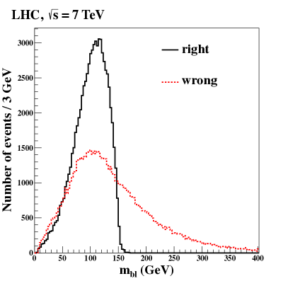
Figure 1: The $m_{b\ell}$ distribution for the $t\bar{t}$ event topology (1) with right (solid black) and wrong (red dashed) partitions of the $b$ quarks and charged leptons. The event generation details for this and the rest of our plots are described in sec. 2.2.

At the level of reconstructed objects, this process is triggered on by, e.g., requiring at least two jets (two of which possibly $b$-tagged), two leptons and missing energy in the final state. Clearly, the triggered-on objects can be partitioned in two different ways, namely

right partition $$\equiv \{\ell_{1}b_{1}\}\&\{\ell_{2}b_{2}\}~{},$$

wrong partition $$\equiv \{\ell_{1}b_{2}\}\&\{\ell_{2}b_{1}\}~{},$$

where the index labels the decay chain. In the rest of the text we will refer to the different ways of grouping visible final states into two sets as partitions.

Our aim is to construct test variables able to distinguish the right from the wrong final-state partitions. To this end, one may exploit suitable event variables, that namely display certain predictable features as a function of the event kinematics – like edges, thresholds or peaks. The main observation to take advantage of is that these features are present, and calculable from the measured final states, provided the partition of the visible particles is the right one, whereas they are partly or completely destroyed if the final-state partition is incorrect.

The arguably simplest and best-known example to illustrate such ideas is the invariant mass of the visible particles, $m_{V_{i}}$, belonging to a given decay chain $i$. In the case of the event topology (1), the visible particles of each decay chain are a $b$-quark and a charged lepton. The corresponding invariant mass distribution enjoys an upper endpoint given by the formula

$$\left(m_{b\ell}^{\rm max}\right)^{2} = m_{b}^{2}+\frac{1}{2}\left(m_{t}^{2}-m_{W}^{2}-m_{b}^{2}\right)+\frac{1}{2}\sqrt{\left(m_{t}^{2}-m_{W}^{2}-m_{b}^{2}\right)^{2}-4m_{W}^{2}m_{b}^{2}}$$ (2)

$$\simeq 153.2\,\mbox{GeV}~{}.$$

This endpoint feature is clearly displayed by the black solid histogram in fig. 1, representing the $m_{b\ell}$ distribution when correctly partitioning the final states. The same feature does not need to hold in case $m_{b\ell}$ is calculated with the incorrect final-state partition: the corresponding histogram is also shown as a red dashed curve. Indicating the two possible partitions as $P_{1}$ and $P_{2}$, one can then construct the difference between the $m_{b\ell}$ values calculated with either partition, namely

$$\Delta T(P_{2},\,P_{1})\equiv T(P_{2})-T(P_{1})~{},$$ (3)

where

$$T(P_{i})\equiv m_{b\ell}(P_{i})$$ (4)

is the test variable for a given partition $P_{i}$. From our previous considerations, one can expect that, if $P_{1}$ corresponds to the right partition, $P_{R}$, and $P_{2}$ to the wrong one, $P_{W}$, then $\Delta T(P_{W},\,P_{R})$ is expected to be larger than zero, at least for a subset of the possible kinematic configurations of the visible final states.

We therefore introduce the following criterion for using $\Delta T(P_{2},\,P_{1})$ as a variable testing the correct final-state partition in the case of dileptonic $t\bar{t}$ decay:

Given a final state of $2b$-jets $+2\ell$, they can be partitioned in two possible ways, to be called $P_{1}$ and $P_{2}$. If $\Delta T(P_{2},\,P_{1})$, defined as eq. (3), is found to be $>0$ ($<0$), then $P_{1}$ ($P_{2}$) may be identified as the correct partition, with a calculable probability $p$ of misidentification.

In the sections to follow we will introduce several such test variables $T(P)$, and for each of them estimate the efficiency $1-p$. We will also see that this efficiency can be systematically improved in two directions:

• by introducing further kinematic cuts on the event sample, at the price of a reduced statistics;

• by combining the information from several $T(P)$ in a global test variable, for example, a likelihood test with the $\Delta T(P_{2},\,P_{1})$ distributions interpreted as probability distributions.

Both of the above points will be addressed in the sections starting from sec. 3. All the numerical results of our paper rely on event simulations, whose details are introduced in the next section 2.2. In the rest of sec. 2 we will introduce all the test variables and discuss variations around their definitions as well as their efficiencies.

2.2 Event generation and selection

We generated 100,000 parton-level events of top quark pair production followed by dileptonic final states using MadGraph 5, with proton-proton collisions at $\sqrt{s}=7$ TeV Alwall:2011uj . We here do not assume any contribution from physics beyond the SM. The SM predicts $\sigma_{t\bar{t}}\sim 162$ pb at next-to-next-to-leading-order Aliev:2010zk . Hence the generated events correspond to $\sim 13$ fb^-1. The dilepton mode gives rise to final states with two $b$-tagged jets, two leptons, missing transverse energy. We consider the leptonic decays of the $W$ bosons to an electron or muon.

We apply event selection cuts on the simulated event sample following the 0.7 fb^-1 ATLAS dileptonic top analysis ATLAS-CONF-2011-100 . We namely require

• exactly two oppositely-charged leptons ($ee$, $\mu\mu$, $e\mu$) with $p_{T}>25$ GeV and $|\eta|<2.5$,

• at least two jets with $p_{T}>25$ GeV and $|\eta|<2.5$,

• dilepton invariant mass, $m_{\ell\ell}>15$ GeV,

• that events in the same-flavor lepton channels must satisfy the missing transverse energy condition ${\hbox to0.0pt{\hbox to7.95831pt{\hfil/\hfil}\hss}E}_{T}>60$ GeV and $|m_{\ell\ell}-m_{Z}|>10$ GeV,

• that events in the different-flavor channel satisfy $H_{T}>130$ GeV. The event variable $H_{T}$ is defined as the scalar sum of the transverse momenta of the two leptons and all selected jets. In analogy with ATLAS-CONF-2011-100 we instead do not require $\hbox to0.0pt{\hbox to7.95831pt{\hfil/\hfil}\hss}E_{T}$ or $m_{\ell\ell}$ cuts in this channel.

We found that about 37% of the total simulated events pass these basic selection cuts. The motivation for including the mentioned cuts is to have an event sample that resembles as much as possible the actual experimental event samples in dileptonic $t\bar{t}$ production. As such, it will be our reference event sample throughout our analysis. We leave aside for the moment the important issues of: inclusion of hadronization, QCD radiation, and modeling of detector effects, that we will address in a forthcoming, more in-depth study futureWork .

2.3 Test variables: definition and discussion

2.3.1 Invariant mass of visible final states: $T_{1}$ variable

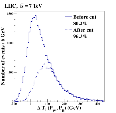
Figure 2: Distribution for the variable $\Delta T_{1}(P_{W},\,P_{R})$ (see defs. in eqs. (6) and (3)) with $P_{W}$ and $P_{R}$ denoting the wrong and the right partition respectively. The legend in the plot indicates the percentage of correctly partitioned events, before and after inclusion of the cut $M_{T}^{t\bar{t}}(0)>400$ GeV, to be described in sec. 3.2.

Our first test variable is constructed from $m_{b\ell}$, mentioned in the example of sec. 2.1. In particular, it could be defined directly as in eq. (4). However, for each event one obtains two $m_{b\ell}$ values, $m_{b\ell}^{(i)}$ $(i=1,\,2)$, corresponding to the two decay chains. Combining the two $m_{b\ell}^{(i)}$ values in different ways gives rises to alternative definitions of the test variable, not all of which yield the same efficiency. We found the combination ${\rm max}[m_{b\ell}^{(1)},\,m_{b\ell}^{(2)}]$ to perform best:

$${\rm max}\left[m_{b\ell}^{(1)},\,m_{b\ell}^{(2)}\right](P_{W})>$$

$$\max\left[m_{b\ell}^{(1)},\,m_{b\ell}^{(2)}\right](P_{R}):80.2\%~{}.$$ (5)

We correspondingly define our first test variable as follows:

$$T_{1}(P_{i})\equiv{\rm max}\left[m_{b\ell}^{(1)},\,m_{b\ell}^{(2)}\right](P_{i})~{},$$ (6)

for a given partition $P_{i}$. The $\Delta T_{1}(P_{W},\,P_{R})$ distribution is shown in fig. 2.

The efficiency figure in eq. (2.3.1), as well as in the solid histogram in fig. 2, refers to the events that pass the basic selection cuts described in sec. 2.2, and actually includes one further consideration: if one of the partitions results in $m_{b\ell}>m_{b\ell}^{\rm max}$, then the right partition can be clearly selected because $m_{b\ell}(P_{R})\leq m_{b\ell}^{\rm max}$.

2.3.2 $M_{T2}$ of the whole decay chain: $T_{2}$ variable

Another event variable that may be used to construct a test variable of correct partitioning is $M_{T2}$, the so-called “stransverse mass”, which is especially suited to topologies with pair-produced particles, each decaying into partly invisible final states Lester:1999tx ; Barr:2003rg . The general event topology that $M_{T2}$ is suited for is the following:

$$Y\bar{Y}~{}\to~{}V_{1}(p_{1})\chi(k_{1})+V_{2}(p_{2})\bar{\chi}(k_{2})~{},$$ (7)

where each of the $V_{i}$ denotes a (set of) visible state(s), whose total four-momentum is, in principle, entirely reconstructible, and $\chi$, $\bar{\chi}$ denote invisible particles with identical mass. The decay mode (1) is an example of this very event topology: $V_{i}$ should be identified with a $b~{}\ell$ pair (for each decay chain) and $\chi,\bar{\chi}$ with the neutrinos.

For the event topology (7), the $M_{T2}$ variable is defined as

$$M_{T2}(\tilde{m}_{\chi})\equiv\min_{\tilde{\bf k}_{{\bf 1}T}+\tilde{\bf k}_{{\bf 2}T}={\bf{\hbox to0.0pt{\hbox to3.52188pt{\hfil/\hfil}\hss}p}}_{T}}\left[\max\left\{M_{T}^{(1)}\left({\bf p_{1}}_{T},\,\tilde{\bf k}_{{\bf 1}T},\,p_{1}^{2},\,\tilde{m}_{\chi}\right),\,M_{T}^{(2)}\left({\bf p_{2}}_{T},\,\tilde{\bf k}_{{\bf 2}T},\,p_{2}^{2},\,\tilde{m}_{\chi}\right)\right\}\right]~{},$$

where $M_{T}^{(i)}$ is the transverse mass Smith:1983aa ; Barger:1983wf of the decay chain $i\,(=1\mbox{ or }2)$, namely

$$\left(M_{T}^{(i)}\right)^{2}=p_{i}^{2}+\tilde{m}_{\chi}^{2}+2\left(\sqrt{|{\bf p_{i}}_{T}|^{2}+p_{i}^{2}}\sqrt{|\tilde{\bf k_{i}}_{T}|^{2}+\tilde{m}_{\chi}^{2}}-{\bf p_{i}}_{T}\cdot\tilde{\bf k_{i}}_{T}\right)~{}.$$ (9)

A few comments may help get an intuitive picture of the above definitions. First, it should be kept in mind that what is measured in the event topology of (7) are the visible particles’ momenta, $p_{i}$, and the total momentum imbalance in the transverse direction, ${\bf\hbox to0.0pt{\hbox to5.03125pt{\hfil/\hfil}\hss}p}_{T}$. The definition in eq. (2.3.2) correspondingly marginalizes over the transverse momenta ${\bf k}_{{\bf 1,2}T}$ of $\chi$, $\bar{\chi}$, that are not separately measured, by taking the minimum over all the trial momentum configurations (denoted with a tilde), whose sum equals the measured ${\bf\hbox to0.0pt{\hbox to5.03125pt{\hfil/\hfil}\hss}p}_{T}$.

Second, the invisible mass $m_{\chi}$ is, likewise, unmeasured, hence $M_{T2}$ is a function of a trial value for this mass, $\tilde{m}_{\chi}$. In the case of the decay (1) $m_{\chi}$ is of course known: $m_{\chi}=m_{\nu}\approx 0$. However, the topology in eq. (7) applies also to several new-physics scenarios, and in this case the physical mass $m_{\chi}$ of the pair-produced $\chi$ is in general unknown. An interesting feature of $M_{T2}$ is the kink structure of $M_{T2}^{\rm max}(\tilde{m}_{\chi})$ at $\tilde{m}_{\chi}=m_{\chi}$, provided the $p_{i}^{2}$ value spans a certain range in each decay chain Cho:2007qv ; Cho:2007dh . An alternative possibility for the kink structure of $M_{T2}^{\rm max}(\tilde{m}_{\chi})$ to appear is to have the $Y\bar{Y}$ system boosted by a sizable amount of upstream transverse momentum Gripaios:2007is ; Barr:2007hy . The $M_{T2}$-kink method makes it possible to measure $m_{\chi}$ and $m_{Y}$ simultaneously, and even if the decay chain is not long enough to constrain all the unknowns in the event.

The property of $M_{T2}$ most relevant to our discussion is that, when the input trial mass $\tilde{m}_{\chi}$ equals the true mass value $m_{\chi}$, the upper endpoint of the $M_{T2}$ distribution corresponds to the parent particle mass $m_{Y}$. We want to use this property to distinguish the correct against the incorrect partition of the final-state visible particles. We note explicitly that, in dileptonic $t\bar{t}$, one can construct two kinds of $M_{T2}$: $M_{T2}^{t\bar{t}}$ for the full $t\bar{t}$ system and $M_{T2}^{WW}$ for the $WW$ subsystem Nojiri:2008vq ; Burns:2008va ; Choi:2010dk ; Choi:2010dw , the visible particles being respectively $b\ell^{+}\bar{b}\ell^{-}$ and $\ell^{+}\ell^{-}$. Since only one partition is possible in $M_{T2}^{WW}$, this variable cannot be used directly as a test variable. It can however be used to construct other test variables, to be introduced in the next section. In the rest of the present discussion we will therefore specialize to $M_{T2}^{t\bar{t}}$.

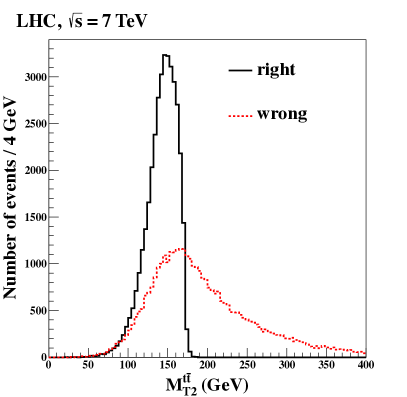
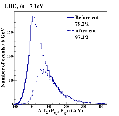
Figure 3: The distributions of $T_{2}\equiv M_{T2}^{t\bar{t}}$ (left panel) and $\Delta T_{2}(P_{W},\,P_{R})$ (right panel), with $P_{W}$ and $P_{R}$ the wrong and right partitions respectively. The legend in the second panel indicates the percentage of correctly partitioned events, before and after inclusion of the cut $M_{T}^{t\bar{t}}(0)>400$ GeV, to be described in sec. 3.2.

As already mentioned, the $M_{T2}^{t\bar{t}}$ distribution is bounded from above by the top quark mass $m_{t}$ if the partition is the right one, whereas it is not if the partition is the wrong one. This fact is shown in the left panel of fig. 3. One can therefore define the variable

$$T_{2}(P_{i})\equiv M_{T2}^{t\bar{t}}(P_{i})~{},$$ (10)

where we recall that $P_{i}$ ($i=1,\,2$) denotes the two possible partitions of the $2b+2\ell$ visible final states.

In the right panel of fig. 3, we show the distribution of $\Delta T_{2}(P_{W},\,P_{R})$ with the right ($P_{R}$) and wrong ($P_{W}$) partitions. The figure shows that the relation $\Delta T_{2}(P_{W},\,P_{R})>0$ holds for about 80% of the events that passed just the basic selection cuts described in sec. 2.2, and that this percentage reaches as much as 97% after the $M_{T}^{t\bar{t}}(0)$ cut to be described in sec. 3.2.

To conclude this section, we mention that the $M_{T2}$ method of finding the right partition has been proven to be useful for mass measurements and/or event reconstruction in refs. Barr:2007hy ; Lester:2007fq ; Cho:2008cu ; Alwall:2009zu ; Aaltonen:2009rm ; Konar:2009qr ; Berger:2010fy ; Nojiri:2010mk ; Zhang:2010kr ; Berger:2011ua ; Park:2011uz ; Murayama:2011hj .

2.3.3 MAOS-reconstructed $m_{t}$ and $m_{W}$ mass: $T_{3,4}$ variables

A further set of variables to test the correct partition can be constructed from the observation that the sum of final-state momenta in either decay chain must reconstruct, up to width effects, the parent-particle’s invariant mass. The main obstacle to this, in the case of the event topology (7), is the fact that the invisible momenta of the two decay chains, $k_{1}$ and $k_{2}$, are not measured separately, but only their sum is, and only in the transverse plane.

Systematic techniques exist however, enabling to obtain a best guess of the invisible momenta $k_{1}$ and $k_{2}$. Among these techniques is the so-called $M_{T2}$-assisted on-shell (MAOS) reconstruction of invisible momenta Cho:2008tj . The only assumption of the MAOS method is that the event topology should be of the kind of eq. (7). Then the transverse components of the invisible momenta, ${\bf k}_{{\bf 1}T}$, ${\bf k}_{{\bf 2}T}$, can be estimated event by event to be the location of the minimum of the $M_{T2}$ variable constructed for the event. Recall in fact that, from eq. (2.3.2), $M_{T2}$ is obtained from a minimization over all possible $\tilde{\bf k}_{{\bf 1,2}T}$ configurations subject to the constraint $\tilde{\bf k}_{{\bf 1}T}+\tilde{\bf k}_{{\bf 2}T}={\bf{\hbox to0.0pt{\hbox to5.03125pt{\hfil/\hfil}\hss}p}}_{T}$.

Once ${\bf k}_{{\bf 1}T}$ and ${\bf k}_{{\bf 2}T}$ are estimated by $M_{T2}$, the longitudinal components of the invisible momenta may be determined from the on-shell relations

$$(p_{i}+k_{i}^{\rm maos})^{2}=m_{Y}^{2}~{},\quad(k_{i}^{\rm maos})^{2}=m_{\chi}^{2}$$ (11)

where, as usual, $i$ labels the decay chain, $m_{Y}$ the parent particle mass, and $m_{\chi}$ the invisible particle mass. Eqs. (11) amount to a quadratic equation in the longitudinal components of $k_{i}$, hence one has in general two solutions for each decay chain, $\tilde{k}_{{\bf i}L}^{\pm}$. Modulo this two-fold ambiguity, and assuming $m_{\chi}$ to be known (in our case it is $m_{\nu}\approx 0$), the MAOS reconstruction thus leads to a estimate of the full invisible momenta $k_{i}$. Specifically, $k_{i}^{\rm maos}$ has a roughly Gaussian distribution around $k_{i}^{\rm true}$ and a moderate spread, that can be systematically improved by requiring event cuts Cho:2008tj .

In our case, the whole argument in the previous paragraph can be applied to the full $t\bar{t}$ decay, or to the $WW$ subsystem, because both share the same, mentioned topology (7). In particular, from the MAOS momenta of the $WW$ system, $k^{{\rm maos}\mbox{-}WW}_{1,2}$, one can construct the invariant mass of the top quark as

$$\left(m_{t,i}^{\rm maos}\right)^{2}\equiv\left(p_{b,i}+p_{\ell,i}+k_{i}^{{\rm maos}\mbox{-}WW}\right)^{2}~{},$$ (12)

whereas from the MAOS momenta of the $t\bar{t}$ system, $k_{i}^{{\rm maos}\mbox{-}t\bar{t}}$, one can construct the $W$ boson invariant mass as

$$\left(m_{W,i}^{\rm maos}\right)^{2}\equiv\left(p_{\ell,i}+k_{i}^{{\rm maos}\mbox{-}t\bar{t}}\right)^{2}~{}.$$ (13)

It is clear that, if the right partition is selected and in the limit where the MAOS momenta equal the true momenta in each decay chain, eqs. (12) and (13) should equal respectively the true $m_{t}$ and $m_{W}$ values, up to finite decay widths. In practice, the MAOS momenta differ in general from the true momenta. However, the MAOS invariant mass distribution exhibits a peak structure around the true parent particle mass. Hence — to the extent that the spread around the peak value is not too large — the above eqs. (12) and (13) are still useful for our purpose, which is, we recall, not to measure the $t$ or $W$ mass, but to single out the correct final-state partition. We show in fig. 4 the $m_{t}^{\rm maos}$ (left panel) and the $m_{W}^{\rm maos}$ (right panel) distributions calculated using the right partition (black solid histogram) and the wrong partition (red dashed histogram).

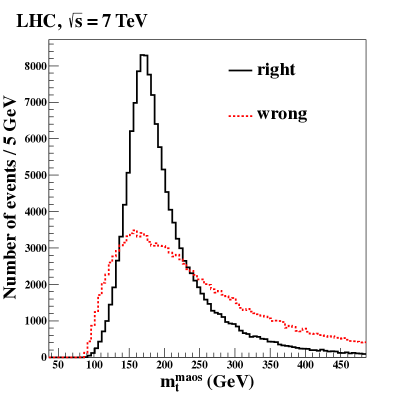
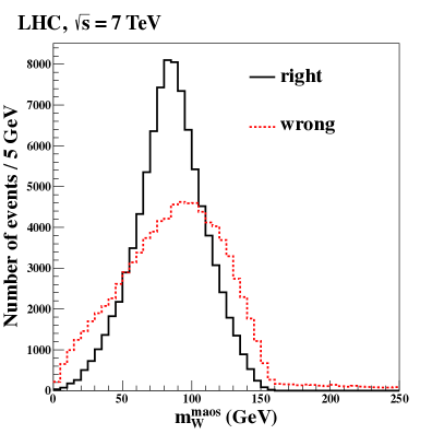
Figure 4: The $m_{t}^{\rm maos}$ (left panel) and $m_{W}^{\rm maos}$ (right panel) distributions for the right and for the wrong final-state partition. The distributions include only events with real MAOS solutions for all partitions (see text for details).

The argument below eqs. (12)-(13) may be used to construct a test variable of correct partition by noting that

$$|m_{t,i}^{\rm maos}-m_{t}|(P_{W})>|m_{t,i}^{\rm maos}-m_{t}|(P_{R})~{},$$ (14)

and a similar inequality holds also for $m_{W}^{\rm maos}$. In reality, the notation in relation (14) is incomplete, because of the mentioned discrete ambiguity in the determination of the longitudinal components of the invisible momenta. This is a common problem for methods attempting to reconstruct invisible momenta, and based on polynomial on-shell equations of degree higher than one. One cannot distinguish the solutions among themselves, even though only one solution corresponds to the true one and the others are redundant.

We construct our test variable treating these solutions in a symmetric way. We first define a quantity

$$\Delta_{t}m_{t}^{\rm maos}(\alpha)\equiv m_{t}^{\rm maos}(p_{b},\,p_{l},\,k^{\alpha})-m_{t}\quad(\alpha=+,\,-)~{},$$ (15)

where we omitted the chain label, and $\alpha$ denotes the two MAOS solutions for the invisible momentum $k^{\rm maos}$ in that decay chain. Thence we found that

$$\sum_{i=1,2;\,\alpha=+,-}|\Delta_{t}m_{t,i}^{\rm maos}(\alpha)|(P_{W})>\sum_{i=1,2;\,\alpha=+,-}|\Delta_{t}m_{t,i}^{\rm maos}(\alpha)|(P_{R}):84.2\%~{},$$ (16)

namely that the sum over chains and over $k^{\pm}$ solutions of the quantity defined in (15) is smaller when calculated on the right partition than on the wrong partition in as much as 84% of the events. Consistently with the discussion in sec. 2.1, we then define our test variable $T_{3}$ as follows:

$$T_{3}(P_{k})\equiv\sum_{i=1,2;\,\alpha=+,-}|\Delta_{t}m_{t,i}^{\rm maos}(\alpha)|(P_{k})~{}.$$ (17)

The whole line of reasoning below eq. (14) can be applied to the $WW$ subsystem as well. Similarly as $m_{t}^{\rm maos}$ in (15) one constructs the difference between $m_{W}^{\rm maos}$ and $m_{W}$ and symmetrizes between decay chains and $k^{\pm}$ solutions. We obtained

$$\sum_{i=1,2;\,\alpha=+,-}|\Delta_{W}m_{W,i}^{\rm maos}(\alpha)|(P_{W})>\sum_{i=1,2;\,\alpha=+,-}|\Delta_{W}m_{W,i}^{\rm maos}(\alpha)|(P_{R}):86.8\%~{},$$ (18)

and we define our test variable $T_{4}$ as

$$T_{4}(P_{k})\equiv\sum_{i=1,2;\,\alpha=+,-}|\Delta_{W}m_{W,i}^{\rm maos}(\alpha)|(P_{k})~{}.$$ (19)

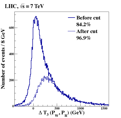
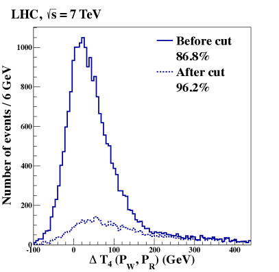
Figure 5: The distributions of $\Delta T_{3}(P_{W},\,P_{R})$ (left panel) and $\Delta T_{4}(P_{W},\,P_{R})$ (right panel), with $P_{W}$ and $P_{R}$ denoting the wrong and the right partition. The legend indicates the percentage of correctly partitioned events, before and after inclusion of the cut $M_{T}^{t\bar{t}}(0)>400$ GeV, to be described in sec. 3.2. The efficiency figures in the right panel take into account the complex-MAOS-solution criterion, whereas histograms report only the events free of complex solutions. See text for full details.

An important difference between the $m_{t}^{\rm maos}$-based method and the $m_{W}^{\rm maos}$-based one should be emphasized. Within the $m_{t}^{\rm maos}$ method, the choice of final-state partition enters only when constructing the top invariant mass (see eq. (12)), whereas only one partition is possible in the estimate of $k_{i}^{{\rm maos}\mbox{-}WW}$. Conversely, within the $m_{W}^{\rm maos}$ method, the choice of final-state partition does come into play in the calculation of $k_{i}^{{\rm maos}\mbox{-}t\bar{t}}$ (see eq. (13)), namely when calculating $M_{T2}$ of the $t\bar{t}$ system. The important point is that wrong partitions sometimes result in complex solutions for (the longitudinal components of) $k_{i}^{{\rm maos}\mbox{-}t\bar{t}}$ much more often than right partitions do, and this can be used as a further criterion for identifying the right partition. From our simulation, we found that:

• events with at least one complex solution (in any of the partitions) occur 38.5% of the time;

• most importantly, events where a complex solution appears only in the wrong partition occur 37.9% of the time – very close to the percentage in point (a).

From the above points, it is clear that the $m_{W}^{\rm maos}$ method can be augmented by the following requirement:

if the MAOS calculation returns at least a complex solution, but only for one of the partitions, then this partition should be regarded as the wrong one.

In the following we will refer to this statement as the complex-MAOS-solution criterion. This requirement has a probability of mistakenly discarding a correctly paired event as small as 5 per mil, as can easily be deduced from the above items. Note that this criterion is already taken into account in the 86.8% efficiency figure reported in eq. (18) and should be regarded as part and parcel of the $\Delta T_{4}$ method.

The whole discussion between eq. (16) and the previous paragraph is illustrated in the plots of fig. 5, that report the distributions for $\Delta T_{3}(P_{W},\,P_{R})$ and $\Delta T_{4}(P_{W},\,P_{R})$ (we recall the reader that $\Delta T$ is defined in eq. (3)). In particular, the efficiency figures in eqs. (16) and (18) correspond to the solid-line histograms, namely those before the $M_{T}^{t\bar{t}}(0)$ cut to be introduced in sec. 3.2 (see figure legend).

A careful reader may have noted that, in the $\Delta T_{4}$ panel, the percentage of events in the positive semiaxis looks, and in fact is, smaller that the corresponding efficiency (percentage of correctly partitioned events) indicated in the legend. This is especially true for the histogram after the $M_{T}^{t\bar{t}}(0)$ cut. The reason is the fact that the $T_{4}$-method efficiency is calculated as the sum of the $\Delta T_{4}>0$ criterion and, when applicable, of the complex-MAOS-solution criterion, that by itself belongs to the $T_{4}$-method, as already mentioned. Schematically, the total $T_{4}$-method efficiency, $\epsilon_{T_{4}}$, splits up as follows:

$$\epsilon_{T_{4}}~{}=~{}C\cdot\epsilon_{C}+R\cdot\epsilon_{R}~{},$$ (20)

where $C$ is the percentage of events with complex solutions, $R$ is the percentage of events free of complex solutions ($C+R=$100%), $\epsilon_{C}$ denotes the efficiency of the complex-MAOS-solutions method and $\epsilon_{R}$ the efficiency of the $\Delta T_{4}>0$ method. For the events passing the $M_{T}^{t\bar{t}}(0)$ cut, we found $R=31\%$ and $\epsilon_{R}\simeq 90\%$. The $R$ subset is the only one displayed in the dashed histogram on the right panel of fig. 5, and the efficiency $\epsilon_{R}$ is the percentage of this histogram lying in the positive semiaxis. More importantly for the overall method efficiency $\epsilon_{T_{4}}$ in eq. (20) is to note that $C=1-R=69\%$ and that $\epsilon_{C}\simeq 99\%$, to be compared with $C=38.5\%$ (and $\epsilon_{C}$ basically the same) before the cut. These figures demonstrate that, after the cut, wrongly partitioned events tend to display complex MAOS solutions way more often than before the cut. This behavior is actually expected: if the $T_{4}$ variable, constructed with wrongly partitioned kinematics, may produce complex solutions, they will tend to proliferate if the kinematics gets more boosted, as is the case after the cut. The bottom line is that, from the point of view of the overall $T_{4}$-method efficiency, an increase in the number of events with complex solutions $C$ is an advantage, because the complex-MAOS-solution criterion has by itself an efficiency $\epsilon_{C}$ of nearly 100% of picking up the correct partition.

To conclude this section, we note explicitly that the previous discussion refers to events at parton level, as assumed throughout this paper. Of course, effects such as momentum smearing may well destabilize the above conclusions. However, it seems reasonable to believe that the main effect of smearing will not be to have complex solutions migrate from the wrong to the right partition, but rather to increase the number of events where both the right and wrong partitions consist of only complex solutions. Such events represented only 0.6% of our total events (see point (b) above), and we simply did not use the $T_{4}$ variable for such events. It is possible that this fraction of events increases, maybe even substantially, when including mismeasurement effects. Rather than simply disposing of the $T_{4}$ variable for these events, one may instead consider introducing some more general complex-solution criterion than the one advocated in this section. One such criterion may be to choose as the true partition the one whose MAOS solution has, for instance, the largest real part. It is worth mentioning that the issue of complex solutions in event reconstruction has been recently discussed in detail in ref. Gripaios:2011jm , and the argument in the present paragraph is inspired by the main messages in that paper. We leave the question of the utility and efficiency of our thus-reformulated complex-MAOS-solution criterion to forthcoming work futureWork where smearing effects will be taken into account.

3 Improving the method efficiency

3.1 Correlations and combinations of the test variables

In the previous section we have shown that each of the introduced test variables $T_{i}$ is able to find the correct final-state partition in $\gtrsim 80$% of the total events that pass the basic selection cuts. Already at the end of section 2.1 we have emphasized that the overall method efficiency may be systematically improved by combining the $T_{i}$ and/or by introducing appropriate kinematic cuts. We will now address these two possibilities in turn.

First of all, the possibility that combining the $T_{i}$ does indeed allow to increase the overall method efficiency relies on the $T_{i}$ being as weakly correlated as possible. Hence, we should first address the question of how large these correlations are. For the reader’s convenience, we recall that our $T_{i}$ are defined in eqs. (6), (10), (17) and (19) and that we also introduced a complex-MAOS-solution criterion at the end of sec. 2.3.3. Two-dimensional plots of the $\Delta T_{i}(P_{W},\,P_{R})-\Delta T_{j}(P_{W},\,P_{R})$ correlations are shown in fig. 6. These plots do not include events with complex solutions.

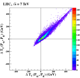
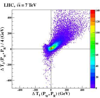
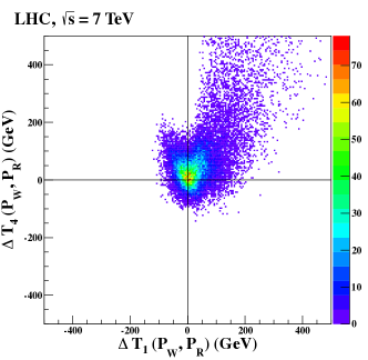
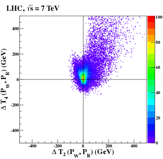
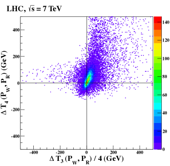
Figure 6: Plots of the correlations between $\Delta T_{i}(P_{W},\,P_{R})$ and $\Delta T_{j}(P_{W},\,P_{R})$. The color code refers to the number of events in each plot pixel.

The following comments are in order. First, it is apparent that $T_{1}$ and $T_{2}$ have a quite strong correlation. This is because the $m_{b\ell}$ value is directly used in the calculation of $M_{T2}$, that is a monotonically increasing function of $m_{b\ell}$. Further, the MAOS-related variables, $T_{3}$ and $T_{4}$, are expected to have some degree of correlation with respectively $T_{1}$ (related to $m_{b\ell}$) or $T_{2}$ (related to $M_{T2}^{t\bar{t}}$). Arguments in support of this statement go as follows. Concerning the $T_{3}-T_{1}$ correlation, $m_{t}^{\rm maos}$ was defined as

$$\left(m_{t}^{\rm maos}\right)^{2}=m_{b\ell}^{2}+2\left(\sqrt{(m_{b\ell})^{2}+|{\bf p}_{b\ell}|^{2}}|{\bf k}^{{\rm maos}\mbox{-}WW}|-{\bf p}_{b\ell}\cdot{\bf k}^{{\rm maos}\mbox{-}WW}\right),$$

whence the dependence on $m_{b\ell}$ is apparent. With regards to the $T_{4}-T_{2}$ correlation, recall instead that the $m_{b\ell}$ value was used when calculating $k^{\rm maos\mbox{-}t\bar{t}}$, in turn necessary for $m_{W}^{\rm maos}$. However, in practice, these correlations turn out to be rather weak, and this occurs because of the nontrivial structure of the MAOS solutions. For example, if $M_{T2}^{t\bar{t}}$ is calculated from a balanced configuration, $m_{t}^{\rm maos}$ can also be written as

$$\left(m_{t}^{\rm maos}\right)^{2} = m_{b\ell}^{2}+2\left(\sqrt{(m_{b\ell})^{2}+|{\bf p}_{T,b\ell}|^{2}}|{\bf k}_{T}|\cosh(\eta_{b\ell}-\eta_{\nu})-{\bf p}_{T,b\ell}\cdot{\bf k}_{T}\right)$$ (21)

$$= \left(M_{T2}^{t\bar{t}}\right)^{2}+2\sqrt{(m_{b\ell})^{2}+|{\bf p}_{T,b\ell}|^{2}}|{\bf k}_{T}|\left[\cosh(\eta_{b\ell}-\eta_{\nu})-1\right],$$

for given ${\bf k}_{T}$ values. Therefore, we can regard each of $\{T_{3},T_{4}\}$ vs. each of $\{T_{1},T_{2}\}$ as approximately uncorrelated.

In principle, one can merge the information from the various $T_{i}$ even in presence of correlations among them, e.g. by constructing a likelihood function (not to mention more sophisticated pattern-finding techniques such as neural networks). The exploration of optimal ways of using the combined information from all the $T_{i}$ is of course beyond the scope of the present paper. Besides, it should be emphasized that each of the introduced variables can actually be defined in a number of variations. One may adopt the approach of considering all these variations and using their information in a joint way, that properly takes into account correlations. This approach would also offer a way to improve the method efficiency. We refrain from entertaining such approach in this paper, which is devoted to the discussion of the main ideas behind each variable.

Here we limit ourselves to show that even a very simple combination of the test variables results in an appreciable improvement of the overall method efficiency. We choose $\{T_{2},\,T_{3},\,T_{4}\}$ as a set of independent test variables. Then, the arguably simplest algorithm to find the right partition by using these variables in a combined test is as follows:

• Calculate $T_{2}$, $T_{3}$ and $T_{4}$ for the two possible partitions: $P_{1}$ and $P_{2}$;

• If $T_{1}(P_{i})>m_{b\ell}^{\rm max}$ or $T_{2}(P_{i})>m_{t}$, regard $P_{i}$ as the wrong partition;

• If $T_{4}(P_{i})$ results in complex MAOS solutions, whereas no complex solutions are present for the other partition, regard $P_{i}$ as the wrong partition;

• If none of the above criteria is met, then choose $P_{1}$($P_{2}$) as the right partition if the majority of $\Delta T_{i}(P_{2},\,P_{1})>0$ ($<0$).

Point 1 corresponds to the already mentioned, and well-known, observation that $m_{b\ell}$ and $M_{T2}^{t\bar{t}}$ have a physical upper bound at $m_{bl}^{\rm max}$ and $m_{t}$ respectively, if the partition is the correct one. Point 2 is the complex-MAOS-solution criterion enunciated at the end of sec. 2.3.3. As also discussed there, this method selects the right partition for $98.4\%$ of the events with at least one complex solution. According to our simulation, the combined algorithm 0-3 described above returns the right partition for 89% of the full data set, which we find an already remarkable improvement over the single-variable efficiency.

3.2 Improving by cuts on kinematic variables

Up to this point, we have not introduced any event selection cuts, except for the basic cuts described in sec. 2.2, that, we checked, have only a marginal impact on the $T_{i}$ efficiencies. Although the previous section shows that a method efficiency of 90% or even larger is arguably obtainable by just a wise combination of the $T_{i}$, we would like to show in this section that improvements are possible also by imposing appropriate kinematic variable cuts. This of course comes at the price of losing (some) event statistics.

First, we note that the property of the test variables of being larger when evaluated with the wrong partition becomes more marked as the final states are more energetic. Intuitively, the larger the magnitude of the input kinematics, the more spread becomes the distribution of the variable, if it is calculated with the wrong partition. On the other hand, the distribution calculated with the right partition enjoys the same physical endpoints independently, of course, of the input kinematics. So, for a more boosted subset of events, one expects $\Delta T_{i}(P_{W},P_{R})$ to be larger than zero more often. To single out such event subset, one may enforce cuts on appropriate kinematic variables, and parametrically improve the method efficiency as the cut gets stronger.

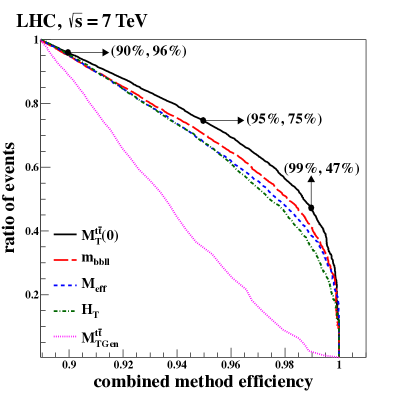
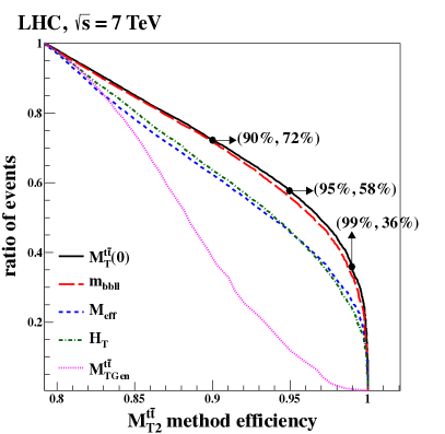
Figure 7: (Left panel) Combined method efficiency vs. loss in statistics with the inclusion of an inclusive cut. The $x$-axis represents the efficiency of the combined method described in sec. 3.1 whereas the $y$-axis reports the number of events that passed one of the inclusive cuts, listed with different line/color codes in the legend. Events are normalized to the event subset that passed the basic selection cuts discussed in sec. 2.2. (Right panel) Same as the left panel, but for the $T_{2}$ variable only, rather than the combined method, on the $x$-axis.

For the dileptonic $t\bar{t}$ process, a well-known set of ‘partition-insensitive’ kinematic variables – which namely treat all the visible particles on an equal footing, hence they are free of combinatorial ambiguities – is represented by:

• $M_{T}^{t\bar{t}}(0)$,

• $m_{V}^{2}\equiv(p_{b_{1}}+p_{b_{2}}+p_{\ell_{1}}+p_{\ell_{2}})^{2}$,

• $M_{\rm eff}=\sum_{i}p_{{\bf i}T}+|{\bf\hbox to0.0pt{\hbox to5.03125pt{\hfil/\hfil}\hss}p}_{T}|$,

• $H_{T}=\sum_{i}p_{{\bf i}T}$, where $i=b_{1},\,b_{2},\,\ell_{1},\,\ell_{2}$,

• $M_{T{\rm Gen}}^{t\bar{t}}$,

where $M_{T}^{t\bar{t}}(0)$ is the transverse mass of the full $t\bar{t}$ system with $m_{\nu\nu}=0$ Park:2011uz ; Barr:2009mx ; Tovey:2010de ,

$$\left(M_{T}^{t\bar{t}}(0)\right)^{2}\equiv m_{V}^{2}+2\left(\sqrt{|{\bf p}_{T}|^{2}+m_{V}^{2}}|{\bf\hbox to0.0pt{\hbox to5.03125pt{\hfil/\hfil}\hss}p}_{T}|-{\bf p}_{T}\cdot{\bf\hbox to0.0pt{\hbox to5.03125pt{\hfil/\hfil}\hss}p}_{T}\right)\quad\mbox{with }{\bf p}\equiv\sum_{i=b,\,\ell}{\bf p}_{i}~{},$$ (22)

and $M_{T{\rm Gen}}^{t\bar{t}}$ is the smallest value of $M_{T2}^{t\bar{t}}$ obtained over all possible partitions Lester:2007fq . One can impose these cuts in addition to the basic event selection cuts of sec. 2.2. In the left panel of fig. 7, we show the flow of method efficiency vs. loss in statistics as one makes the cuts harder. See figure caption for full details.

The figure shows that the most effective cut variable is $M_{T}^{t\bar{t}}(0)$. One can reach 90% method efficiency (i.e. get the right partition 90% of the times) with just a 4% loss in event statistics. The efficiency rises to 99% when roughly halving the statistics. For the sake of completeness, we also mention that, for the quoted efficiencies of 90%, 95% and 99%, the cut value is respectively $M_{T}^{t\bar{t}}(0)>$ 277, 343 and 404 GeV.

Because, for some event topologies to be described in the next section, the MAOS-based variables $T_{3}$ and $T_{4}$ are not usable, but the $M_{T2}$-based variable $T_{2}$ still is, we also show in the right panel of fig. 7 a plot of efficiency gain vs. statistics loss for the $T_{2}$ variable alone.

4 Generalizations of the method

4.1 Case of chain-assignment as well as ordering ambiguities

From the discussion so far, our method of finding the right partition can be promptly generalized, in particular to topologies relevant for new physics scenarios. Among the most popular such event topologies is the one in eq. (7), that is, pair-production of heavy particles, decaying into a set of visible particles plus a pair of invisible particles (possibly, dark-matter candidates). We here sketch this generalization, leaving full details to future work futureWork . For the sake of discussion, we here focus on identical decay chains, but the argument presented below can be extended also to the case of non-identical decay chains.

The first observation to make is that the decay of heavy parent particles can be in one step or multiple steps, depending on the mass spectrum and couplings of the new particles. The $T_{1}$ and $T_{2}$ variables of secs. 2.3.1 and 2.3.2 can be defined, and applied to find the right partition of the visible particles, even in the case of a one-step decay, e.g., gluino-pair production, followed by the three-body decay $\tilde{g}\to qq\tilde{\chi}_{1}^{0}$ in $R$-parity conserving supersymmetric models.

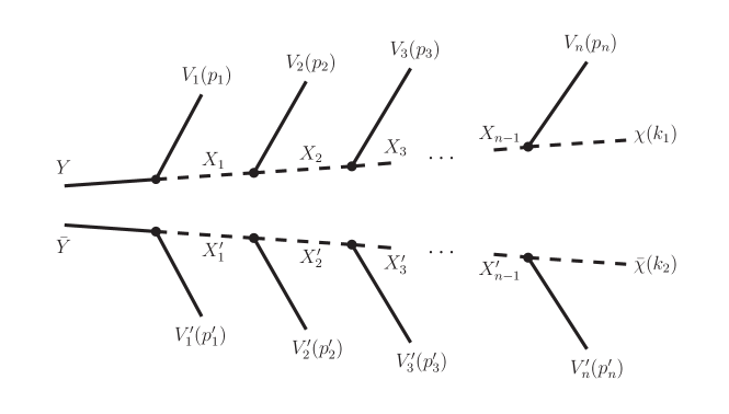
Figure 8: The decay process of eq. (23). The momenta $p_{i}$ and $p^{\prime}_{i}$ are assumed to be measurable, while $k_{i}$ give rise to missing transverse momentum.

On the other hand, to utilize the MAOS-based variables $T_{3}$ and $T_{4}$, the decay process should be at least in two steps, as e.g. the dileptonic $t\bar{t}$ process is. For instance, if $m_{\tilde{q}}<m_{\tilde{g}}$, gluino-pair production will be dominantly followed by two-step decays, i.e., $\tilde{g}\to q\tilde{q}\to qq\tilde{\chi}_{1}^{0}$. In terms of event topology, the cascade decay processes of interest to this discussion can be generalized as

$$Y\bar{Y} \to V_{1}(p_{1})X_{1}+V_{1}^{\prime}(p_{1}^{\prime})X_{1}^{\prime}\to V_{1}(p_{1})V_{2}(p_{2})X_{2}+V_{1}^{\prime}(p_{1}^{\prime})V_{2}^{\prime}(p_{2}^{\prime})X_{2}^{\prime}$$ (23)

$$\to \cdots\to V_{1}(p_{1})\cdots V_{n}(p_{n})\chi(k_{1})+V_{1}^{\prime}(p_{1}^{\prime})\cdots V_{n}^{\prime}(p_{n}^{\prime})\bar{\chi}~{}(k_{2})~{},$$

for $m_{Y}>m_{X_{1}}>m_{X_{2}}>\cdots>m_{\chi}$ and $m_{\bar{Y}}>m_{X_{1}^{\prime}}>m_{X_{2}^{\prime}}>\cdots>m_{\bar{\chi}}$. This decay is also sketched in fig. 8. The rest of the present discussion will also assume $m_{X_{i}}=m_{X_{i}^{\prime}}$, albeit this requirement is renounceable with appropriate modifications of the method.

The second observation is that, in the context of this general event topology, there is, when partitioning the visible particles, an additional type of combinatorial ambiguity with respect to dileptonic $t\bar{t}$. It is the ordering ambiguity, corresponding to the fact that $V_{a}^{(\prime)}$ is produced before $V_{a+1}^{(\prime)}$ ($a=1,\,\cdots,\,n-1$). Of course, there is still, as in dileptonic $t\bar{t}$, the combinatorial ambiguity of pairing the visible particles into two sets, i.e., distinguishing $\{V_{a}\}$ from $\{V_{a}^{\prime}\}$. Then, the total number of partitions of the visible particles is

$$N=(\mbox{number of pairings})\times(\mbox{number of orderings in one chain})^{2}=\frac{{}_{2n}C_{n}}{2}\times(n!)^{2}~{},$$ (24)

if the visible particles are not distinguishable among each other, as is the case for jets (barring taggings etc.). Then, one can calculate the MAOS invariant masses of $2n$ parent particles ($Y,\,X_{1},\,\cdots,\,X_{n-1},\,\bar{Y},\,X_{1}^{\prime},\cdots,\,X_{n-1}^{\prime}$), such that $n$ MAOS-based test variables are defined. We will label them as $T_{a}^{\rm maos}$ ($a=0,\,\cdots,\,n-1$), for a given partition $P_{j}$ ($j=1,\,\cdots,\,N$) and MAOS momenta $k^{\rm maos}$ (we recall that the MAOS determination of the invisible momenta consists in general of several solutions, collectively indicated as $k^{\rm maos}$). Thence, one can define:

$$T_{a}^{\rm maos}(P_{j},\,k^{\rm maos})\equiv\sum_{c=1,2;\,\alpha=+,-}|\Delta_{X_{a}}m_{X_{a}}^{\rm maos}(p_{a\,c},\,k_{c}^{\alpha})|(P_{j})~{},$$ (25)

where

$$\Delta_{X_{a}}m_{X_{a}}^{\rm maos}(p_{a\,c},k_{c}^{\alpha})\equiv m_{X_{a}}^{\rm maos}(p_{a\,c},\,k_{c}^{\alpha})-m_{X_{a}}$$ (26)

with $p_{a\,1}\equiv\sum_{j=a+1}^{n}p_{j}$, $p_{a\,2}\equiv\sum_{j=a+1}^{n}p_{j}^{\prime}$, and $X_{0}=Y$. These correspond to the $T_{3}$ and $T_{4}$ variables discussed in sec. 2.3.3. Actually, each $T_{a}^{\rm maos}(P_{j},\,k^{\rm maos})$ can be obtained in different ways, since the MAOS momenta $k^{\rm maos}$ can be calculated from ${}_{n}C_{2}$ subsystems. In order to account for them in a symmetric way, one may define $T_{a}^{\rm maos}$ as

$$T_{a}^{\rm maos}(P_{j})\equiv\sum_{\forall k^{\rm maos}}T_{a}^{\rm maos}(P_{j},\,k^{\rm maos})~{}.$$ (27)

Each $T_{a}^{\rm maos}$ variable can then be used to decide on the right partition: this partition is likely to have the smallest $T_{a}^{\rm maos}$ value than all the other partitions, irrespective of whether combinatorial ambiguities concern the pairing or the ordering of the visible particle sets.

The $T_{1}$ and $T_{2}$ variables are also usable because one can calculate several subsystem $T_{1}$’s and $T_{2}$’s. For example, in the event topology (23), the subsystem $T_{2}$, or briefly $T_{2}^{\rm sub}$, can be defined as $T_{2}^{Y\bar{Y}},\,T_{2}^{X_{1}X_{1}^{\prime}},\,\cdots,\,T_{2}^{X_{n-1}X_{n-1}^{\prime}}$, such that $T_{2}^{Y\bar{Y}}\leq m_{Y},\,T_{2}^{X_{1}X_{1}^{\prime}}\leq m_{X_{1}}$, $\cdots$, $T_{2}^{X_{n-1}X_{n-1}^{\prime}}\leq m_{X_{n-1}}$ for the right partition. By sequentially testing the partitions in the order $Y\bar{Y}\to\cdots\to X_{n-1}X_{n-1}^{\prime}$ systems, at each step selecting the partition with the smallest $T_{2}^{\rm sub}$, one can find the most likely partition for the full system.

We finally observe that the information from the above test variables can be merged into a combined method in various ways. The simplest algorithm may be

• Calculate all the test variables as explained above. If $T_{1}^{X_{a}X_{a}^{\prime}}>m^{\rm max}_{V_{a+1}\cdots V_{n}}=m_{V_{a+1}^{\prime}\cdots V_{n}^{\prime}}^{\rm max}$ or $T_{2}^{X_{a}X_{a}^{\prime}}>m_{X_{a}}$ for $a=0,\,\cdots,\,n-2$ or there are more complex MAOS solutions in a given partition $P_{j}$ than in any other partition, one should regard $P_{j}$ as the wrong one.

• If the above procedure fails to pick up one partition, one may select the right partition $P_{j}$ from the requirement that it gives the smallest value of $T_{i}$ (with respect to the other partitions) for the largest number of test variables.

We again emphasize that the efficiency of each $T_{i}$ and of the combined method can be further improved by imposing cuts on ‘partition-insensitive’ variables, as discussed in sec. 3.2.

Concrete examples of this generalized method will be the gluino pair-production and decay discussed above, and the pair-production of the second lightest neutralino $\tilde{\chi}_{2}^{0}$, which decays to $\ell^{+}\ell^{-}\tilde{\chi}_{1}^{0}$. We will consider in more details these new physics processes for certain benchmark points in future work futureWork .

4.2 Comments about the method’s dependence on mass information

We would like to conclude this section about generalizations with a few remarks about the question of the method’s dependence on the knowledge of the mass of the pair-produced states, $m_{Y}$, or that of the invisible daughters, $m_{\chi}$. As a first remark, we emphasize again that, of our proposed $T_{i}$, the variables $T_{1}$ as well as $T_{2}$ do not use the information on $m_{Y}$ at all. On the other hand, this information appears necessary for constructing the MAOS-based variables $T_{3}$ and $T_{4}$, at least according to the way they were defined in sec. 2.3.3. In order to be able to use the variables $T_{3,4}$ at all, one would therefore seem to need $m_{Y}$ and $m_{\chi}$ to have been measured already.

It is worth observing that, in many scenarios of new physics, the mass measurements in question are not expected to be affected by combinatorial ambiguities. This holds in particular in the case of the topologies of interest for our method, where one can construct the event variable $M_{T2}$. In fact, if, in absence of combinatorial ambiguities, $m_{Y}$ may be estimated from the endpoint of $M_{T2}$, then, in presence of combinatorial ambiguities, the same estimate can be performed using $M_{T{\rm Gen}}$ Lester:2007fq instead, i.e. the smallest $M_{T2}$ value for all possible partitions, which enjoys the same endpoint position as $M_{T2}$ constructed with the right partition. In cases where the production cross-section is so small, or background contamination so high, that the mass information cannot practically be extracted along the above lines, one can consider using a modified version of our MAOS-based variables, wherein the parametric dependence on the true value of $m_{Y}$ is disposed of. To make an example, in place of the $T_{3}$ definition, given in eq. (17), one may instead use the quantity

$$\tilde{T}_{3}(P_{k})~{}\equiv~{}|m_{t}^{\rm maos}(\mbox{chain 1})-m_{t}^{\rm maos}(\mbox{chain 2})|~{},$$ (28)

which should be close to zero if the partition is the correct one, whereas it can be much larger if the partition is wrong. Hence, again, $\Delta\tilde{T}_{3}(P_{W},P_{R})$ is expected to prefer positive values. We note explicitly that the notation in eq. (28) is, similarly as in eq. (14), incomplete, in that the MAOS solution obtained from the on-shell relations (11) is not unique (see discussion below those relations). On the other hand, on the r.h.s. of eq. (11), one does not necessarily have to choose the parent particle mass. One has in general the following choices Park:2011uz

• MAOS1: $m_{Y}$ Cho:2008tj

• MAOS2: $M_{T2}={\rm min}_{\vec{p}_{\chi_{1},T}+\vec{p}_{\chi_{2},T}=\hbox to0.0pt{\hbox to6.5382pt{\hfil/\hfil}\hss}\vec{p}_{T}}~{}{\rm max}\{M_{T}^{(1)},M_{T}^{(2)}\}$

• MAOS3: $M_{T}^{(i)}$, with $i=1,2$ labeling the decay chain.

The advantage of MAOS3 is that it allows to have a unique MAOS solution for each event, thereby allowing use of the $\tilde{T}_{3}$ variable as defined in eq. (28). In fact, we found the performance of $\Delta\tilde{T}_{3}$ comparable to that of $\Delta T_{3}$, as defined in sec. 2.3.3. The reason why we defined our MAOS-based variables according to the MAOS1 scheme is mostly simplicity.

The other unknown mass besides $m_{Y}$ is $m_{\chi}$, upon which all the $T_{i}$ variables bear dependence. While the necessity to input some $m_{\chi}$ value seems inescapable, we are actually quite confident that our method would perform rather well even in the case where the $m_{\chi}$ mass is yet to be measured at the moment of having to solve the combinatorial problem. We make the following considerations in support of this statement. First, as already mentioned in the general $M_{T2}$ discussion in sec. 2.3.2, an estimate, perhaps an accurate one, of $m_{\chi}$ may be obtained from the $M_{T2}$ kink Cho:2007qv ; Cho:2007dh ; Gripaios:2007is ; Barr:2007hy , which however requires sufficient statistics. Even in absence of such statistics, and in presence of combinatorial ambiguities, the uppermost part of the $M_{T{\rm Gen}}(m_{\chi})$ plot in the $m_{\chi}$ vs. $m_{Y}$ plane may provide a rough idea of the $m_{\chi}$ mass. It is worth emphasizing that a rough input value for $m_{\chi}$ may well be sufficient in many scenarios. It is so at least in the case where $m_{\chi}\ll m_{Y}$: it can be shown in fact Kiwoon_unpub that, in this limit, MAOS solutions have corrections going as $m_{\chi}^{2}/m_{Y}^{2}$ and are, therefore, largely insensitive to the specific value chosen for $m_{\chi}$, so long as the mentioned mass hierarchy holds at least approximately.

Clearly, all the issues mentioned in this section deserve further investigation, which is best carried out within specific new-physics benchmark points. This lies outside the scope of the present paper, mainly meant to propose our method and to apply it to the simplest yet relevant SM example we could think of, namely $t\bar{t}$ production. We will however return to all these issues in a forthcoming paper futureWork .

5 Conclusions and Outlook

In this paper, we have proposed a novel method to resolve combinatorial ambiguities in hadron collider events involving two invisible particles in the final state. This method is based on the kinematic variable $M_{T2}$ and on the MAOS reconstruction of invisible momenta, that are reformulated as test variables $T_{i}$, namely testing the correct combination against the incorrect ones. The efficiency of each single $T_{i}$ in the determination of the correct combination can then be systematically improved in two directions: by combining the information from the different $T_{i}$ and by introducing further cuts on suitable, partition-insensitive, variables. In this sense, our method is completely scalable.

All the above program is illustrated in the specific, and per se interesting example of top anti-top production, followed by a leptonic decay of the $W$ on both sides. We however emphasize that, by construction, our method is also directly applicable to many topologies of interest for new physics, in particular events producing a pair of undetected particles, that are potential dark-matter candidates.

Our method opens a whole spectrum of generalizations and by-product issues, on which work is in progress futureWork . The most urgent include:

• Addressing whether and how the method is affected by the inclusion of effects such as QCD radiation, hadronization and signal degradation due to detector effects. The main challenge of this problem is that, after hadronization, the assignment of a ‘parton’ to a given decay chain or to a certain position within the decay chain is no more well-defined. As such, it requires separate thought.

• Generalizing the method to the combinatorial uncertainty due to the ordering of the visible particles in the decay chain, uncertainty which is not present in dileptonic $t\bar{t}$.

- (1) A. J. Barr and C. G. Lester, A Review of the Mass Measurement Techniques proposed for the Large Hadron Collider, J.Phys.G G37 (2010) 123001, [arXiv:1004.2732].
- (2) A. Rajaraman and F. Yu, A New Method for Resolving Combinatorial Ambiguities at Hadron Colliders, Phys.Lett. B700 (2011) 126–132, [arXiv:1009.2751].
- (3) G. Mahlon and S. J. Parke, Angular correlations in top quark pair production and decay at hadron colliders, Phys.Rev. D53 (1996) 4886–4896, [hep-ph/9512264].
- (4) T. Stelzer and S. Willenbrock, Spin correlation in top quark production at hadron colliders, Phys.Lett. B374 (1996) 169–172, [hep-ph/9512292].
- (5) G. Mahlon and S. J. Parke, Maximizing spin correlations in top quark pair production at the Tevatron, Phys.Lett. B411 (1997) 173–179, [hep-ph/9706304].
- (6) G. Mahlon and S. J. Parke, Spin Correlation Effects in Top Quark Pair Production at the LHC, Phys.Rev. D81 (2010) 074024, [arXiv:1001.3422].
- (7) C. Lester and D. Summers, Measuring masses of semiinvisibly decaying particles pair produced at hadron colliders, Phys.Lett. B463 (1999) 99–103, [hep-ph/9906349].
- (8) A. Barr, C. Lester, and P. Stephens, : The Truth behind the glamour, J.Phys.G G29 (2003) 2343–2363, [hep-ph/0304226].
- (9) W. S. Cho, K. Choi, Y. G. Kim, and C. B. Park, -assisted on-shell reconstruction of missing momenta and its application to spin measurement at the LHC, Phys.Rev. D79 (2009) 031701, [arXiv:0810.4853].
- (10) J. Alwall, M. Herquet, F. Maltoni, O. Mattelaer, and T. Stelzer, MadGraph 5 : Going Beyond, JHEP 1106 (2011) 128, [arXiv:1106.0522].
- (11) M. Aliev, H. Lacker, U. Langenfeld, S. Moch, P. Uwer, et. al., HATHOR: HAdronic Top and Heavy quarks crOss section calculatoR, Comput.Phys.Commun. 182 (2011) 1034–1046, [arXiv:1007.1327].
- (12) P. M. Nadolsky, H.-L. Lai, Q.-H. Cao, J. Huston, J. Pumplin, et. al., Implications of CTEQ global analysis for collider observables, Phys.Rev. D78 (2008) 013004, [arXiv:0802.0007].
- (13) Atlas Collaboration, Measurement of the top quark pair production cross section in collisions at tev in dilepton final states with atlas, Tech. Rep. ATLAS-CONF-2011-100, CERN, Geneva, Jul, 2011.
- (14) K. Choi, D. Guadagnoli and C. B. Park, in preparation.
- (15) J. Smith, W. van Neerven, and J. Vermaseren, The transverse mass and width of the boson, Phys.Rev.Lett. 50 (1983) 1738.
- (16) V. D. Barger, A. D. Martin, and R. Phillips, Perpendicular e neutrino mass from decay, Z.Phys. C21 (1983) 99.
- (17) W. S. Cho, K. Choi, Y. G. Kim, and C. B. Park, Gluino Stransverse Mass, Phys.Rev.Lett. 100 (2008) 171801, [arXiv:0709.0288].
- (18) W. S. Cho, K. Choi, Y. G. Kim, and C. B. Park, Measuring superparticle masses at hadron collider using the transverse mass kink, JHEP 0802 (2008) 035, [arXiv:0711.4526].
- (19) B. Gripaios, Transverse observables and mass determination at hadron colliders, JHEP 0802 (2008) 053, [arXiv:0709.2740].
- (20) A. J. Barr, B. Gripaios, and C. G. Lester, Weighing Wimps with Kinks at Colliders: Invisible Particle Mass Measurements from Endpoints, JHEP 0802 (2008) 014, [arXiv:0711.4008].
- (21) M. M. Nojiri, K. Sakurai, Y. Shimizu, and M. Takeuchi, Handling jets + missing channel using inclusive , JHEP 0810 (2008) 100, [arXiv:0808.1094].
- (22) M. Burns, K. Kong, K. T. Matchev, and M. Park, Using Subsystem for Complete Mass Determinations in Decay Chains with Missing Energy at Hadron Colliders, JHEP 0903 (2009) 143, [arXiv:0810.5576].
- (23) K. Choi, D. Guadagnoli, S. H. Im, and C. B. Park, Sparticle masses from transverse-mass kinks at the LHC: The Case of Yukawa-unified SUSY GUTs, JHEP 1010 (2010) 025, [arXiv:1005.0618].
- (24) K. Choi, J. S. Lee, and C. B. Park, Measuring the Higgs boson mass with transverse mass variables, Phys.Rev. D82 (2010) 113017, [arXiv:1008.2690].
- (25) C. Lester and A. Barr, : Mass scale measurements in pair-production at colliders, JHEP 0712 (2007) 102, [arXiv:0708.1028].
- (26) W. S. Cho, K. Choi, Y. G. Kim, and C. B. Park, Measuring the top quark mass with at the LHC, Phys.Rev. D78 (2008) 034019, [arXiv:0804.2185].
- (27) J. Alwall, K. Hiramatsu, M. M. Nojiri, and Y. Shimizu, Novel reconstruction technique for New Physics processes with initial state radiation, Phys.Rev.Lett. 103 (2009) 151802, [arXiv:0905.1201].
- (28) CDF Collaboration, T. Aaltonen et. al., Top Quark Mass Measurement using in the Dilepton Channel at CDF, Phys.Rev. D81 (2010) 031102, [arXiv:0911.2956].
- (29) P. Konar, K. Kong, K. T. Matchev, and M. Park, Dark Matter Particle Spectroscopy at the LHC: Generalizing to Asymmetric Event Topologies, JHEP 1004 (2010) 086, [arXiv:0911.4126].
- (30) E. L. Berger, Q.-H. Cao, C.-R. Chen, G. Shaughnessy, and H. Zhang, Color Sextet Scalars in Early LHC Experiments, Phys.Rev.Lett. 105 (2010) 181802, [arXiv:1005.2622].
- (31) M. M. Nojiri and K. Sakurai, Controlling ISR in sparticle mass reconstruction, Phys.Rev. D82 (2010) 115026, [arXiv:1008.1813].
- (32) H. Zhang, E. L. Berger, Q.-H. Cao, C.-R. Chen, and G. Shaughnessy, Color Sextet Vector Bosons and Same-Sign Top Quark Pairs at the LHC, Phys.Lett. B696 (2011) 68–73, [arXiv:1009.5379].
- (33) E. L. Berger, Q.-H. Cao, C.-R. Chen, C. S. Li, and H. Zhang, Top Quark Forward-Backward Asymmetry and Same-Sign Top Quark Pairs, Phys.Rev.Lett. 106 (2011) 201801, [arXiv:1101.5625].
- (34) C. B. Park, Reconstructing the heavy resonance at hadron colliders, Phys.Rev. D84 (2011) 096001, [arXiv:1106.6087].
- (35) H. Murayama, M. Nojiri, and K. Tobioka, Improved discovery of nearly degenerate model: MUED using at the LHC, arXiv:1107.3369.
- (36) D0 Collaboration, B. Abbott et. al., Measurement of the top quark mass using dilepton events, Phys.Rev.Lett. 80 (1998) 2063–2068, [hep-ex/9706014].
- (37) D0 Collaboration, V. M. Abazov et. al., Measurement of the top quark mass in final states with two leptons, Phys.Rev. D80 (2009) 092006, [arXiv:0904.3195].
- (38) D0 Collaboration, V. M. Abazov et. al., Measurement of spin correlation in production using dilepton final states, Phys.Lett. B702 (2011) 16–23, [arXiv:1103.1871].
- (39) http://www.hep.phy.cam.ac.uk/~lester/mt2/index.html.
- (40) B. Gripaios, K. Sakurai, and B. Webber, Polynomials, Riemann surfaces, and reconstructing missing-energy events, JHEP 1109 (2011) 140, [arXiv:1103.3438].
- (41) A. J. Barr, B. Gripaios, and C. G. Lester, Measuring the Higgs boson mass in dileptonic W-boson decays at hadron colliders, JHEP 0907 (2009) 072, [arXiv:0902.4864].
- (42) D. R. Tovey, Transverse mass and invariant mass observables for measuring the mass of a semi-invisibly decaying heavy particle, JHEP 1011 (2010) 148, [arXiv:1008.3837].
- (43) W. S. Cho, K. Choi and C. B. Park, unpublished.