Precision measurements of the top quark mass from the Tevatron in the pre-LHC era

Abstract

The top quark is the heaviest of the six quarks of the Standard Model. Precise knowledge of its mass is important for imposing constraints on a number of physics processes, including interactions of the as yet unobserved Higgs boson. The Higgs boson is the only missing particle of the Standard Model, central to the electroweak symmetry breaking mechanism and generation of particle masses. In this Review, experimental measurements of the top quark mass accomplished at the Tevatron, a proton-antiproton collider located at the Fermi National Accelerator Laboratory, are described. Topologies of top quark events and methods used to separate signal events from background sources are discussed. Data analysis techniques used to extract information about the top mass value are reviewed. The combination of several most precise measurements performed with the two Tevatron particle detectors, CDF and DØ, yields a value of ${\it M}_{\mbox{\scriptsize\,t}}=173.2\pm 0.9$ GeV/$c^{2}$.

Angela Barbaro Galtieri
Ernest O. Lawrence Berkeley National Laboratory, Berkeley, California 94720
Fabrizio Margaroli
Purdue University, West Lafayette, Indiana 47907
Igor Volobouev
Texas Tech University, Lubbock, Texas 79409

1 Introduction

The Standard Model of Particle Physics unifies the weak and electromagnetic forces into a single quantum field theory. The addition of Quantum Chromodynamics (QCD), which describes the strong interactions that bind quarks into protons and neutrons, completes the Standard Model (SM). The elements of this unified theory are six quarks, six leptons and five gauge bosons. The gauge bosons are the $W^{\pm}$ and $Z$ (carriers of the weak force), the photon (carrier of the electromagnetic force) and the gluon (carrier of the strong force). An additional neutral scalar boson, the Higgs boson, is necessary to explain electroweak (EWK) symmetry breaking, i.e., the observation of non-zero masses of the $W^{\pm}$ and $Z$ bosons. It also generates quark and lepton masses through the Yukawa interaction. A recent review of EWK symmetry breaking scenarios can be found in an earlier issue of this journal [1].

The top quark is the heaviest fundamental fermion. Prior to its direct observation, its mass was predicted through a fit to a number of EWK observables sensitive to virtual top quark effects. This prediction, however, had a very large uncertainty (for historical details, see a plot of top mass expectations and measurements versus time in [2]). The mass of the still unobserved Higgs boson, $M_{\mbox{\scriptsize\,H}}$, is related within the electroweak theory to the $W$ boson mass, $M_{\mbox{\scriptsize\,W}}$, and the top quark mass, $M_{\mbox{\scriptsize\,t}}$, through quantum loop corrections. Some of the lowest order diagrams that link $M_{\mbox{\scriptsize\,W}}$, $M_{\mbox{\scriptsize\,t}}$, and $M_{\mbox{\scriptsize\,H}}$ are shown in Figure 1.

Figure 1: Lowest order diagrams that correlate $M_{\mbox{\scriptsize\,W}}$, $M_{\mbox{\scriptsize\,t}}$, and $M_{\mbox{\scriptsize\,H}}$.

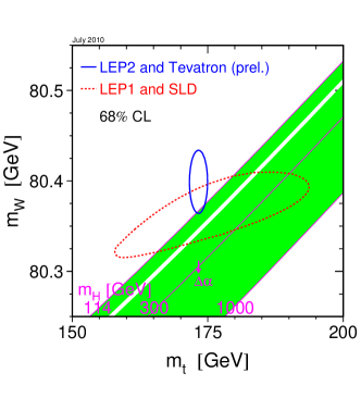
Precision measurements of the masses of the $W$ boson and the top quark are essential to predict the mass of the Higgs boson. An overall fit of EWK observables including the $W$ and the top masses can put constraints on the Higgs mass [3]. Figure 2 illustrates the relationship between the three masses, given current measurements. The Standard Model fit of 18 EWK observables (without the mass measurements) constrains the Higgs mass to lie inside the dashed contour, while the precision with which the $W$ and top masses are currently known constrains the Higgs mass to the smaller solid contour. From the latter we see that a change of 1 GeV/$c^{2}$ in the top mass shifts the predicted central value of the Higgs mass by $\sim 10$ GeV/$c^{2}$.

Figure 2: The relationship between M${}_{\mbox{\scriptsize\,W}}$, ${\it M}_{\mbox{\scriptsize\,t}}$, and M${}_{\mbox{\scriptsize\,H}}$. For each value of M${}_{\mbox{\scriptsize\,H}}$, the Standard Model constraints possible values of $M_{\mbox{\scriptsize\,W}}$ and ${\it M}_{\mbox{\scriptsize\,t}}$ so that they have to lie along the corresponding diagonal band. The dashed contour is the indirect constraint on M${}_{\mbox{\scriptsize\,W}}$ and ${\it M}_{\mbox{\scriptsize\,t}}$ from measurements of 18 EWK observables; the solid contour is the expectation from the M${}_{\mbox{\scriptsize\,W}}$ and ${\it M}_{\mbox{\scriptsize\,t}}$ direct measurements. All contours are for the 68% CL fit result [3].

The discovery of the bottom quark in 1977 [4] set in motion the search for its partner in the third fermion doublet. Experimental lower limits on the top mass slowly increased from a few GeV/$c^{2}$ until the top quark was observed and its mass was directly measured at the Tevatron 18 years later [5, 6]. A first hint for the top quark was reported by the CDF collaboration in [7], together with a mass value of $174\pm 10\pm 13$ GeV/$c^{2}$. Today, the measured value of the top quark mass is not very far from this very early estimate. Increased statistics, better understanding of detector performance, and better measurement techniques have reduced the uncertainty considerably.

The top quark is much heavier than its partner, the bottom quark, whose mass is about $5$ GeV/$c^{2}$ (see [8] for a review on quark masses). The Yukawa coupling of the top quark, $\lambda_{t}$ = 2^3/4 G${}_{F}^{1/2}{\it M}_{\mbox{\scriptsize\,t}}$, is of order unity. This raises the question if the top quark is distinct from the other quarks, i.e., does it have a special role in the electroweak symmetry breaking? A dynamical breaking of EWK theory by a top quark condensate was proposed even before the top quark was discovered [9], later extended to a topcolor model [10]. So far no experimental evidence for the validity of such a model has been found.

1.1 Top mass definition

When referring to quark masses, it is important to define which theoretical framework is used for the given value of the mass. For example, in the overall fit of electroweak measurements the top quark mass needs to be expressed in the ${\overline{MS}}$ renormalization scheme. It is not completely clear how to relate the mass measured in $t\bar{t}$ production experiments with the mass used in the EWK fit. It is normally assumed that what is being measured is the pole mass, $M_{\mbox{\scriptsize\,pole}}$. The relation between $M_{\mbox{\scriptsize\,pole}}$ and the mass in the ${\overline{MS}}$ scheme, $M_{\overline{MS}}$, can be computed within perturbative QCD. Using approximate next-to-next-to-leading order (NNLO) calculations, the difference is about 10 GeV/$c^{2}$, the ${\overline{MS}}$ mass being smaller [11, 12].

The top quark mass can be determined from a measurement of the total $t\bar{t}$ production cross section. The cross section dependence on the mass can be calculated in any renormalization scheme, and the results for the ${\overline{MS}}$ scheme are given in [11]. The DØ collaboration has extracted a top mass in the ${\overline{MS}}$ scheme from such a measurement [13], but the precision of this method is not comparable with that achieved by direct top mass measurements from the top decay products, with a subsequent change from $M_{\mbox{\scriptsize\,pole}}$ to $M_{\overline{MS}}$.

A number of theoretical questions arise in relating the mass measured directly to the pole mass [12, 14]. First, the pole mass is sensitive to an infrared renormalon, which implies that the value of the pole mass is modified by an amount of the order of $\Lambda_{\mbox{\scriptsize\,QCD}}$ as the order in perturbation theory is changed [15]. Second, there are some doubts as to the precise definition of the measured mass. The direct measurements reported here are all calibrated with Monte Carlo generators, therefore what is measured is the mass parameter used in the generators, $M_{\mbox{\scriptsize\,MC}}$. The relationship between $M_{\mbox{\scriptsize\,pole}}$ and $M_{\mbox{\scriptsize\,MC}}$ can be represented in the general form [12, 16]:

$$M_{\mbox{\scriptsize\,pole}}=M_{\mbox{\scriptsize\,MC}}+Q_{0}[\alpha_{s}(Q_{0})c_{1}+...],$$

where the coefficient $c_{1}$ is not known (it depends on parton shower implementation details in each particular generator), but likely to be of the order unity. The main question is what the appropriate value of the scale $Q_{0}$ should be. It has been argued [12] that the cutoff on radiation in the parton shower evolution of order 1 GeV employed by generators like PYTHIA [17] implies that $Q_{0}$ is of order 1 GeV as well. The difference between the measured mass and the pole mass would then be $\cal{O}$(1 GeV/$c^{2}$). Furthermore, it is not clear if other approximations used in the parton shower development alter the resulting mass, as discussed in Appendix C of [16]. Theoretical studies of this problem are in progress along the lines presented in [18]. It is expected that the relation between $M_{\mbox{\scriptsize\,MC}}$ and $M_{\mbox{\scriptsize\,pole}}$ will be understood in the not too distant future.

1.2 Notation

In the subsequent text, we refer to a number of kinematic and physics quantities. The most common ones are denoted by the following symbols:

$\eta$ — Pseudorapidity which characterizes direction of a vector (e.g., particle momentum) with respect to the colliding beam axis (the z axis). It is related to the vector polar angle, $\theta$, by $\eta=-\ln\left[\tan(\theta/2)\right]$.

$\phi$ — Azimuthal angle of a vector.

$\Delta R$ — Distance in the $\eta$-$\phi$ space: $\Delta R=\sqrt{\Delta\eta^{2}+\Delta\phi^{2}}$. Equation $\Delta R<c$, with respect to a certain direction and with some constant $c$, defines a circle in the $\eta$-$\phi$ space. In the context of jet reconstruction algorithms, such circle is usually referred to as a “cone”.

$p_{T}$ — Transverse momentum: $p_{T}=p\sin\theta$, where $p$ is the momentum magnitude.

$E_{T}$ — Transverse energy, usually defined by $E_{T}=E\sin\theta$, where $E$ is the particle energy.

${\not}{E_{T}}$ — Missing transverse energy. It approximates the transverse momentum carried away by neutrinos in the assumption of a fully hermetic particle detector.

$H_{T}$ — Scalar sum of the $E_{T}$ of all charged leptons and jets in the event added to the ${\not}{E_{T}}$.

M${}_{\mbox{\scriptsize\,t}}$ — Experimentally measured mass of the top quark. Unless noted otherwise, ${\it M}_{\mbox{\scriptsize\,t}}\equiv M_{\mbox{\scriptsize\,MC}}$.

$m_{t}$ — An estimate of the top quark mass obtained in a single collider event.

$\int\mathcal{L}dt$ — Integrated luminosity accumulated by an experiment. $\mathcal{L}$ is the instantaneous luminosity.

2 Top production and decay

A precision measurement of the top quark mass relies heavily on the SM predictions for top production and decay processes. It is therefore essential to validate underlying physics and detector response models by comparing experimental measurements with theoretical expectations. Any deviations found will have to be understood and properly represented in the models. Effects not taken into account explicitly are treated as sources of systematics uncertainties (as discussed in Section 6).

2.1 Cross section for $t\bar{t}$ production

The production of top-antitop pairs is a process that can be calculated in perturbative QCD. Figure 3 illustrates some of the leading order (LO) QCD diagrams that contribute to $t\bar{t}$ production. At the Tevatron, the process is dominated by the quark annihilation diagram (leftmost in the figure), whereas the gluon fusion diagrams contribute only 15% of the total cross section [19, 20]. In contrast, at LHC energies the gluon diagrams are expected to contribute more than the quark diagrams.

Figure 3: Some of the Feynman diagrams that contribute to $t\bar{t}$ production.

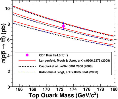
The top cross section measured by CDF at the Tevatron ($\sqrt{s}$ = 1.96 GeV/$c^{2}$) as a function of the top quark mass is shown in Figure 4 [21]. The calculations were performed at NLO+NLL (next-to-leading log) order (Cacciari et al.) [22], at NLO+NNLL (next-to-next-to-leading log) at NLO and approximate NNLO by (Langenfeld et al.) [11] and by (Kidonakis et al.) [23]. The measurement point is placed at ${\it M}_{\mbox{\scriptsize\,t}}$ = 172.5 GeV/$c^{2}$ because this mass value was used to model $t\bar{t}$ production [24]. This measurement, $\sigma_{t\bar{t}}=7.50\pm 0.48$ pb, is the most precise at the time of this writing. It is in a good agreement with the SM calculations.

Figure 4: Top cross section vs. top quark mass as calculated by different authors [11, 22, 23]. For each computation, the middle curve shows the central value for the theoretical prediction, while the upper and lower curves show the $\pm 1\sigma$ computations respectively; the curves from the last two authors are very similar. The data point [21] is the average of two CDF measurements which use the $Z$ boson production cross section to eliminate the luminosity systematics [24].

Measured properties of $t\bar{t}$ events are in agreement with SM expectations (see recent reviews of Tevatron top-quark physics results [25, 26] for more details). Latest confirmations include the correlation between the spins of the top and antitop quarks [27, 28], the fraction of gluon-gluon contribution to the $t\bar{t}$ production cross section [29], and measurements of the $t\bar{t}$ differential cross sections [30, 31] (see Section 4 for a plot). One known exception is the forward-backward asymmetry in top and antitop directions. Recent measurements by both CDF [32] and DØ [33] differ by $\sim 3$ standard deviations from the SM expectation calculated at NLO [34] and approximate NNLO [35]. This anomalous effect is currently under further investigation.

2.2 Top decay modes

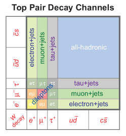
Within the Standard Model, the expected top quark width is $\sim 1.3$ GeV and its lifetime is about $0.5\times 10^{-24}$ seconds. With such a short lifetime ($\ll 1/\Lambda_{\mbox{\scriptsize\,QCD}}$), top quark decays before hadronizing. Observation of its decay products allows for a direct measurement of its mass, a unique feature among quarks [8]. The top quark is expected to decay almost exclusively into a $W$ boson and a bottom quark, so that the intermediate state of a $t\bar{t}$ event is $W^{+}bW^{-}{\bar{b}}$. Each of the two $W$ bosons decays further into a charged lepton and a neutrino or into a quark-antiquark pair (multiple flavor and color assignments are possible), as illustrated in Figure 5. The quarks produced in $W$ decays are not observed as such, but they hadronize producing jets of particles which are subsequently observed and measured in the detectors. At leading order, 10.6% of the $t\bar{t}$ events will have two charged leptons (e, $\mu$, $\tau$), two neutrinos and two jets; 43.9% of the final states will have one charged lepton, one neutrino and four jets, and 45.5% will have six jets. Neutrinos escape direct detection but their presence can be inferred via an excess of missing transverse energy in the event. While $W\rightarrow\ell\nu_{\ell}$ decays, with $\ell=e$ or $\mu$, result in unambiguous experimental signatures, the case $W\rightarrow\tau\nu_{\tau}$ is more complicated as tau leptons subsequently decay in a variety of ways. According to the number of electrons and muons produced in the $W$ decay chains, the final states (“topologies”) of the $t\bar{t}$ system that lead to distinct experimental signatures are called “dilepton”,“$\ell$+jets”, and “all-hadronic”. Taking into account $\sim 35$% leptonic decay branching fraction of the $\tau$, only 6.4% of the events end up in the dilepton category. Similar considerations affect the $\ell$+jets topology which accounts for 34.1% of the events when hadronic $\tau$ decays are excluded.

Figure 5: Final states of the $t\bar{t}$ system.

Measurements of branching fractions of top quark decays [36, 37] have confirmed that the top quark decays predominantly into $Wb$, as predicted by the SM. A number of decay modes of the top quark have been searched for and excluded: decay to a charged Higgs boson (at the level of 10%) and decays through Flavor Changing Neutral Currents (at the level of $10^{-4}$), as summarized in the recent reviews [25, 26]. Other properties of top quarks and their decays, such as $W$ boson helicity fractions [38, 39], top charge [40], and top width [41, 42], have been studied as well, and no significant deviations from the SM expectations have been found.

3 Identifying top events

Stringent requirements are imposed on detectors used for precision measurements of the top quark mass. High resolution charged particle tracking together with high granularity, precise energy determination in calorimeters is necessary for both lepton and jet measurements. Muon momentum measurements and identification are accomplished, in addition to good tracking, with dedicated muon systems located outside the calorimeters. Jet energy measurements require precision calorimetry and good segmentation, as jet shapes play an important role both in the ${\not}{E_{T}}$ measurement and in disambiguation between quark and gluon jets (see Section 7.2). Hermeticity is essential for the ${\not}{E_{T}}$ measurement. High resolution tracking is also needed to identify bottom jets, in particular by reconstructing secondary vertices in jets. Backgrounds to $t\bar{t}$ production are considerably reduced by requiring $b$-jet presence in the event (see Section 3.5).

3.1 Detectors

The CDF detector took its first data in 1985, whereas the DØ detector took its first data in 1992. The top quark was discovered in 1995 and the first direct top mass measurements were made with the initial configuration of these detectors (Tevatron Run I measurements). Both the detectors and the Tevatron accelerator complex went through major upgrades during the 2000-2001 shutdown. Precision measurements of the top mass were performed with the upgraded detectors installed for Run II at the Tevatron.

The Run II CDF detector is shown in Figure 6 [43].

Figure 6: The CDF detector componenents from the collision point outward: the silicon system (purple), the central outer tracker (inner part in orange), the solenoid (yellow), the electromagnetic (red) and hadronic (blue) calorimeters, and the the muon chambers (green) [43].

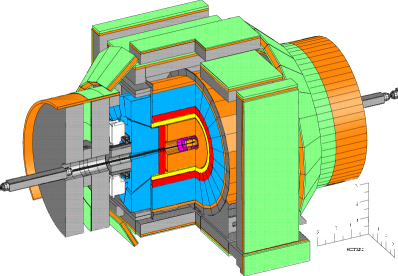
Precision tracking is achieved with: large number of points along the track, high precision space point measurements, long lever arm, and closeness to the production vertex for precision impact parameter determination. Placement of silicon detectors in close vicinity of the beam pipe has allowed CDF to achieve a single-particle transverse momentum determination precision $\frac{\sigma(p_{T})}{p_{T}}=0.07\%p_{T}$ when the primary vertex is included in the track fit [44]. The CDF tracking system consists of a silicon microstrip detector and an open-cell drift chamber immersed in a 1.4 T solenoidal magnetic field. The silicon detector (SVXII) consists of five double sided cylindrical layers of detectors augmented by an inner layer mounted on the beam pipe and two more layers on the outside. They provide precise charged particle tracking in the radial range from 1.5 to 28 cm. Outside this region, the Central Outer Tracker (COT) extends the tracking system to 137 cm providing 96 additional points for track reconstruction. In combination, the COT and the silicon detectors provide excellent tracking up to a pseudorapidity $|\eta|\sim$ 1.0. Additional layers of silicon detectors extend tracking coverage to $|\eta|\sim$ 2.

The central electromagnetic (CEM) calorimeter contains $X_{0}>$ 18 radiation lengths of lead-scintillator layers. Proportional chambers embedded at a depth of $\sim 6X_{0}$ (shower maximum) provide shower shape information for electron identification. The resolution of the CEM calorimeter for electron measurements is $\frac{\sigma(E_{T})}{E_{T}}=\frac{13\%}{\sqrt{E_{T}}}\oplus 1.5\%$. Projective geometry is used: dense segmentation in the CEM, coarser in the hadronic calorimeter. The central hadronic calorimeter is composed of alternating layers of iron plates and scintillators for a total of 4 nuclear interaction lengths. This gives a resolution for charged pions $\frac{\sigma(E_{T})}{E_{T}}=\frac{50\%}{\sqrt{E_{T}}}\oplus 3\%$. In the forward region (1$<|\eta|<$ 3.6) a tile calorimeter is used, with an electron resolution $\frac{\sigma(E)}{E}=\frac{16\%}{\sqrt{E}}\oplus$ 1.0% for the electromagnetic component and a pion resolution $\frac{\sigma(E)}{E}=\frac{80\%}{\sqrt{E}}\oplus 5\%$ for the hadronic component. An additional hadronic calorimeter covers the region between the the central calorimeter and the plug calorimeter, thus providing hermeticity of the detector. Its resolution is $\frac{\sigma(E_{T})}{E_{T}}=\frac{75\%}{\sqrt{E}}\oplus 4\%$ for charged pions that do not interact in the CEM [45].

The muon chambers coverage extends only to $|\eta|<$ 1.0. In the center, two muon detectors cover the $|\eta|<$ 0.6 region. They consist of four layers of proportional chambers each, with the magnet return yoke in between them, thus providing an additional 60 cm of steel absorber. An additional set of four layers of drift chambers cover the region 0.6 $<|\eta|<$ 1.0.

The DØ detector is shown schematically in Figure 7 [46, 47].

Figure 7: The DØ detector [46].

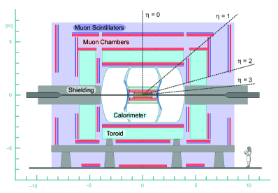
The tracking system consists of a silicon microstrip tracker and a central fiber tracker inside a 2 T solenoid. The silicon detector includes four layers of single and double sided detectors in the central region. In 2006 an additional layer of silicon sensors was added on the beam pipe (the data before and after this addition are identified as Run IIa and Run IIb). In the forward direction disks equipped with silicon detectors complete the tracking system. Outside of the silicon detector system, 16 layers of scintillating fibers (8 axial and 8 stereo), placed in the radial region 20-52 cm, provide additional tracking information. The combination of the tracking devices provides efficient tracking up to pseudorapidity $|\eta|<$ 3. Tracking resolution is $\frac{\sigma(p_{T})}{p_{T}}=0.2\%p_{T}\oplus 1.4\%$.

A preshower detector is placed outside of the magnet and inside the calorimeter. The DØ calorimeter is a Uranium-Liquid-Argon system inside a cryostat. It consists of a central and two endcap components. The EM part has a depth of $\sim$ 20 radiation lengths. The energy resolution for electrons is $\frac{\sigma(E)}{E}=\frac{15\%}{\sqrt{E}}\oplus 4\%$ in the central calorimeter. In the End Cup calorimeter the resolution is $\frac{\sigma(E)}{E}=\frac{21\%}{\sqrt{E}}\oplus 4\%$  [48]. The depth of the hadronic section varies from 7.2 nuclear interaction lengths ($\lambda$) at $|\eta|$ = 0 to $\lambda$ = 10.3 at $|\eta|$ = 1. The calorimeter extends to $|\eta|$ = 4 with a region of low efficiency at $1.0<|\eta|<1.4$.

The muon system surrounds the calorimeter and consists of tracking detectors and scintillators covering a pseudorapidity region up to $|\eta|=1.0$. A toroidal 1.7 T iron magnet completes the central muon system. The forward muon system covers the region 1.0 $<|\eta|<$ 2.0. It consists of mini drift chambers and two toroidal magnets with 1.6 T average field.

Both CDF and DØ use a three-level trigger system to select the events to analyze. The Tevatron delivers collisions to the detectors every 396 ns, which means, at the present luminosity ($\sim 3\times 10^{32}$ cm^-2 s^-1), about $2.5\times 10^{6}$ bunch crossings per second, with an average of five collisions per crossing. The first level hardware trigger reduces the event rate to $\sim 10$ kHz/2 kHz (CDF/DØ). The second level uses trigger processors that reduce the rate to 200 Hz/1000 Hz (CDF/DØ). Finally, the third level is based on limited event reconstruction that reduces the rate to 40 Hz/50 Hz (CDF/DØ). Digitized detector readouts for the accepted events are stored on tape for subsequent offline analysis.

The two detectors have adequate capabilities to perform many precision measurements as well as to explore the vast physics landscape at hand.

3.2 Lepton identification

Electron, muon and neutrino (${\not}{E_{T}}$) reconstruction utilizes event information from all detector subsystems. Electrons are identified using the tracking system ($p_{T}$), the electromagnetic calorimeter ($E_{T}$), the electromagnetic shower shape, and the information from the hadronic calorimeter. CDF obtains the shower shape information from proportional chambers located at shower maximum [43], whereas DØ uses information from finely segmented layers in the liquid argon calorimeter [49]. Electrons that are likely to come from photon conversions are removed using appropriate algorithms. Both experiments have requirements on the $E/p$ ratio to reduce backgrounds from QCD jets. For electrons coming from $W$ decays, an isolation requirement is imposed after all other information is processed. This requirement, which helps in rejecting jets faking electrons, consists in vetoing significant additional energy in a cone of $\Delta R=0.4$ radius around the electron direction. For both experiments, there are several levels of electron criteria: “tight”, “medium”, and “loose”, but most of the top mass measurements use the “tight” electron requirements. Both experiments use $Z\rightarrow e^{+}e^{-}$ decays to calibrate the electron energy.

Muons are identified using information from the muon chambers, the tracking system, and the calorimeters. Having found a signal in the muon chambers, a “muon stub”, i.e., a track segment, is reconstructed. Next step is to match this segment to a track found in the tracking system that extrapolates to the muon chambers within a small distance of the segment. This distance is different for the different components of the muon system for both CDF [43] and DØ [49], as it depends on the resolutions of the chambers and the tracking system as well as on the distance between them. The track is also required to originate from the event primary vertex. The energy deposited in the EM and hadronic calorimeters by the muon is subject to requirements that are different for the two experiments. For muons produced in $W$ decays, a calorimeter isolation as well as a track isolation is required in both experiments. Muons from cosmic rays are removed. The absolute energy calibration is obtained with $Z\rightarrow\mu^{+}\mu^{-}$ decays.

The missing transverse energy, ${\not}{E_{T}}$, is determined from the transverse momentum imbalance in the event. It is calculated by adding vectorially all the calorimeter towers, with the direction defined by the vector connecting the primary vertex to the center of the tower. Corrections to this sum are made for jets and muons in the event. The muon correction is obtained by subtracting the energy deposited by the muon in the calorimeter and by adding its track momentum to the vectorial sum of the tower energies. The energy of the jets in the event is corrected by various coefficients, as described in the next section, and the ${\not}{E_{T}}$ vector is readjusted to take this correction into account.

3.3 Jet reconstruction and calibration

Hadronic jets in $t\bar{t}$ events are reconstructed from the energy flow data collected by the CDF and DØ respective calorimeters. Initially, all energy depositions are grouped into projective “towers” whose size is consistent with the hadronic calorimeter granularity. All towers associated with identified electrons are excluded, electronic noise is subtracted. The remaining towers are clustered into jets using seeded variations of the iterative cone algorithm [50] (which is known as the “mean shift” algorithm [51] in the pattern recognition literature). Although a number of deficiencies have been discovered in the cone-based approach to jet reconstruction [52, 53], extensive studies of various particle processes performed with this algorithm resulted over time in good understanding of jet properties and in consistent calibrations. Fixed jet size permits a very simple correction for the presence of underlying event and multiple interactions occurring in a single bunch crossing.

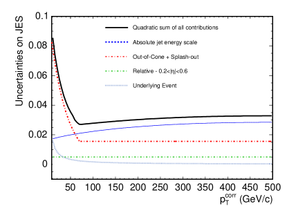
The $\eta$-$\phi$ cone radius used by CDF to reconstruct jets in $t\bar{t}$ events, $\Delta R$ = 0.4, was chosen to optimize efficiency and to minimize energy sharing among different jets. The CDF jet energy resolution is approximately $\sigma(E_{T})$ = (0.1 ($E_{T}$/GeV) + 1.0) GeV for a 0.7 cone radius [45]. The detector response is simulated with the GFLASH parametrization [54] interfaced with GEANT3 [55]. Test beam data, in addition to pion and electron measurements from collider data [56], are used to tune the GFLASH parameters. The $E/p$ distributions at several energies for pions and electrons are compared to the Monte Carlo expectation to obtain the tuning parameters. The jet energy scale is set by the 50 GeV/$c$ test beam data point for pions and by the $Z\rightarrow e^{+}e^{-}$ collider data for electrons. The jets are corrected for non-linear response of the calorimeter; poorly instrumented regions; “multiple interactions”, i.e., the extra energy from the additional collisions occurring in the same bunch crossing (pile-up); “underlying event”, i.e., the energy from the $p\bar{p}$ remnants; and “out-of-cone” energy. After tuning the simulation to the individual particle response, an “absolute” jet correction is derived from simulation. This correction is obtained by comparing the jet $p_{T}$ at the particle level to the jet $p_{T}$ after simulation. The same cone algorithm is used in both cases. The derived correction is valid if the number of tracks and the $p_{T}$ distribution of the tracks in data and in simulations are the same. This was verified using PYTHIA Monte Carlo (MC) samples with jet $p_{T}$ up to 600 GeV/$c$. The uncertainty of this procedure contributes 1% to the jet systematic uncertainty, independent of $p_{T}$. Calibration, done in the central part of the detector (0.2 $<|\eta|<$ 0.6), is extended to all the $\eta$ regions using a dijet imbalance algorithm. Systematic uncertainties arise from uncertainties on the corrections, stability of calorimeter response, calorimeter simulation for EM particles, and calorimeter simulation for hadrons. The different components that contribute to the jet energy scale (JES) uncertainty are shown in Figure 8. The corrections and systematics have been validated using several data samples: dijet, $\gamma$+jets, $Z$+jets, and with hadronic $W$ boson decays in $t\bar{t}$ events [56].

Figure 8: Systematic uncertainties on the jet energy scale for the CDF experiment [56].

The DØ jet energy resolution is $\sigma(E_{T}$) = 9% at 100 GeV for a 0.7 cone radius. The $p_{T}$ dependence is parameterized as $\frac{\sigma(p_{T})}{p_{T}}=\sqrt{\frac{N^{2}}{p_{T}^{2}}+\frac{S^{2}}{p_{T}}+C}$, where $N$ determines the magnitude of the noise term, $S$ is the stochastic term, and $C$ is a constant. The three parameters are evaluated at several $\eta$ intervals [57]. DØ uses the “midpoint” version of the cone algorithm with a radius of 0.5 for top analyses. The multiple interaction correction is determined from events taken with a zero bias trigger during physics data taking. It accounts for noise and energy pile-up. Additional corrections for muons in jets and for radiation outside of the cone are also made. The jet response for jets with $\eta<0.4$ is derived from a high statistics $\gamma$+jets sample, using the $p_{T}$ imbalance of these events. The photon energy scale is assumed to be the same as that of the electrons calibrated with $Z\rightarrow e^{+}e^{-}$ collider data. The extension beyond $\eta=0.4$ is obtained by $p_{T}$ imbalance of dijet events, with one jet in the $\eta<0.4$ region.

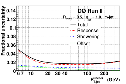
The methods employed for the top mass measurements use jets of particles obtained with Monte Carlo generators followed by a GEANT-based simulation [55]. The jet energy scale is evaluated in the data and in the simulation. The differences are found to be independent from jet $p_{T}$ and $\eta$ and are taken into account in the systematic uncertainties [58, 59]. Figure 9 shows the major components of the systematic uncertainties.

Figure 9: Systematic uncertainties on the jet energy scale for the DØ experiment [46].

Both CDF and DØ use hadronic $W$ decays to determine an overall value of the jet energy scale from the $t\bar{t}$ data, as will be described in more detail in Sections 6 and 7.

3.4 Tagging $b$ jets

One very important ingredient of precision top mass measurements is identification (tagging) of heavy flavor jets. It is essential for suppressing backgrounds from QCD processes as well as for reducing the combinatorics in top events with high jet multiplicity.

Tagging of heavy flavor jets is done in several ways: (a) by identifying muons or electrons originating from bottom or charm hadron decays within the jet; (b) by reconstructing a secondary vertex in jets, due to the decay of a heavy flavor hadrons; (c) by identifying tracks within the jet that originate away from the primary vertex. Most of the top mass measurements performed at the Tevatron use methods (b) and (c) for $b$-jet identification, i.e., use the L${}_{\mbox{\scriptsize\,xy}}$ distance of the secondary vertex or the impact parameter (d₀) of each track, as illustrated in Figure 10.

Figure 10: Secondary vertex reconstruction. L${}_{\mbox{\scriptsize\,xy}}$ is the distance of the secondary vertex from the primary vertex in the plane orthogonal to the proton beam direction. The impact parameter of a track is marked as d₀.

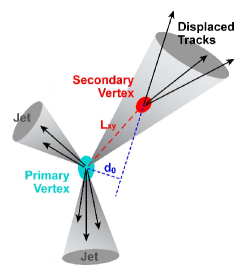
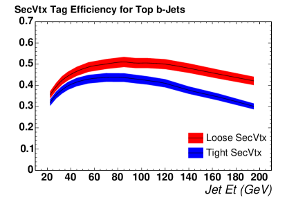
The impact parameter resolution of the CDF tracking system is 35 $\mu$m for tracks with $p_{T}>2$ GeV/$c$ [44]. DØ tracking provides impact parameter measurements with respect to the primary vertex with a precision between 20 and 50 $\mu m$, depending on the number of hits in the silicon detector [60]. The reconstruction of the secondary vertex follows a similar procedure for the CDF [61] and DØ [60] algorithms. A primary vertex for the event is reconstructed using tracks with a small impact parameter significance, $d_{0}/\sigma_{d_{0}}<$ 3. The tracks in jets within a cone of $\Delta R<$ 0.4 (CDF) or 0.5 (DØ) and with large impact parameter significance $d_{0}/\sigma_{d_{0}}>$ 3.5 are used to find a secondary vertex. Additional criteria are set for the significance of the L${}_{\mbox{\scriptsize\,xy}}$ measurement. A jet is tagged as a heavy-flavor jet if all criteria, including a good fit of the secondary vertex, are met. The probability that the displaced vertex is produced by a charm jet is also evaluated, assessing the invariant mass of the tracks that form the secondary vertex. Both MC and data samples are used to evaluate the efficiency of the tagger in top events and the mistag rate, i.e., the probability that a light quark jet is tagged as a heavy flavor jet. The CDF $b$-tagging efficiency as a function of jet $E_{T}$ is shown in Figure 11  [62]. The efficiency for a “tight” $b$-tagging requirement used for the top mass measurements is about 40%. The mistag rate is increasing from 0.4% at 15 GeV to 2.3% at 180 GeV.

Figure 11: The CDF $b$-tag efficiency for “tight” and “loose” $b$-tagging requirements [62]. The average $E_{T}$ of $b$ jets in $t\bar{t}$ events produced at the Tevatron is $\sim 70$ GeV.

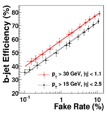
Both CDF and DØ  have developed more sophisticated algorithms for $b$-tagging. They use more information than just the secondary vertex fit result. These neural network (NN) algorithms help reduce the background from light quark jets that mimic heavy flavor jets. The CDF algorithm [63] employs other variables in addition to secondary vertex information, but has not been used for top mass measurements. The DØ NN algorithm [64] was used for top mass measurements. It takes into account information from impact parameter measurements, the secondary vertex tagger, and the soft lepton tagger (SLT). The SLT attempts to identify semileptonic decays within a jet. Separate efficiencies for $b$ and $c$ quark jets as a function of $p_{T}$ and $\eta$ are obtained, and the mistag rate as a function of the same variables is evaluated [64]. The NN is trained on QCD $b\bar{b}$ jets and on light quark Monte Carlo samples, and its performance is measured in data. Figure 12 shows the fake (mistag) rate-vs-efficiency for jets in two different regions of $p_{T}$ and $\eta$.

Figure 12: DØ $b$-tag efficiency vs. fake rate for two $p_{T}$ and $\eta$ regions [60].

3.5 Major background sources

There are two substantially different types of backgrounds: physics processes that have topologies similar to $t\bar{t}$ events and instrumental backgrounds originating from processes that have incompatible final states but can nevertheless appear top-like due to detector imperfections. Physics backgrounds are difficult to eliminate completely, but their rates can be usually reduced by imposing requirements that exploit the differences between signal and background kinematic distributions. Modeling of physics backgrounds is discussed in Section 4.2. Instrumental backgrounds are caused by misidentification of charged leptons, neutrinos (${\not}{E_{T}}$), or $b$ jets. These backgrounds can be reduced by stringent requirements on particle identification criteria (charged leptons), topological cuts for the ${\not}{E_{T}}$ (neutrinos), and sophisticated algorithms for $b$-tagging.

Backgrounds are different for the three major topologies in which the $t\bar{t}$ candidate events are found. A brief description of the major backgrounds in each of these topologies is provided below. Additional details will be given in Section 7, where the actual top mass measurements are discussed.

The background in the dilepton topology (e and $\mu$) is mostly due to Drell-Yan processes ($Z/\gamma^{*}\rightarrow\ell^{+}\ell^{-}$); diboson production: $WW$ and $WZ$ where a lepton from the $Z$ decay is lost and appears as ${\not}{E_{T}}$ (oppositely charged leptons of the same type coming from $Z$ decays are rejected with a $Z$ mass veto); $W+\geq 2$ jets (where one jet mimics an electron or a muon); single top production (lepton +$\geq$ 3 jets where one jet mimics an electron). In addition, “fake” muons can originate from punch-through or from hadrons decaying in flight. Details of instrumental backgrounds for electron and muon identification can be found in [65, 66]. The $t\bar{t}$ decay chains with a $\tau$ lepton are included in the $\ell$+jets or dilepton channels only if the $\tau$ decays leptonically (in $\sim$ 35% of the cases). Studies of the processes involving the $\tau$ lepton are discussed in more detail in Section 7.3.

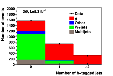
The major background in the $\ell$+jets topology is $W$+jets production which has a much larger cross section than $t\bar{t}$ production. This background is further classified into $W$+light flavor and $W$+heavy flavor. The first one can be reduced considerably by requiring one or more jets to be tagged as a $b$ jet. Another large background (often called non-$W$ QCD) is due to multijet production, where a jet fakes an electron or a muon. Rate estimations for these backgrounds are performed with data driven methods, developed for top cross section measurements. Details can be found in [67, 24] for the CDF analyses and in [64] for DØ analyses. A good review of these methods can be found in [25]. Other instrumental backgrounds are due to mismeasurements of jets which occur in poorly instrumented regions of the detector and increase the value of ${\not}{E_{T}}$. Requiring a certain minimum angle between the jet and the ${\not}{E_{T}}$ direction helps to suppress these backgrounds. Finally, diboson production, i.e., $WW$, $WZ$ and $ZZ$ final states with the same topology as $t\bar{t}$, and single top production also contribute to the background. The dependence of the background rate on the number of $b$-tagged jets can be seen in Figure 13. See Section 7.1 for the contributions of each of these backgrounds to the candidate event samples after application of all selection requirements.

Figure 13: Number of candidate $t\bar{t}$ events vs. the number of tagged jets in the $\ell$+jets topology for events with at least four energetic jets [68].

QCD multijet production is the major background in the all-hadronic topology. Without $b$-tagging requirements, this background is three orders of magnitude larger than the signal. The sample signal fraction is significantly improved by demanding that at least two jets are tagged as a $b$ jet. Additional kinematic requirements, e.g., a neural network selection which combines a number of discriminating variables, are used to suppress the background further, as described in Section 7.2.

Table 1 shows the signal-to-background ratio (S/B) for simple event selection criteria as a rough estimate. For the dilepton and $\ell$+jets channels: $E_{T}(leptons)>20$ GeV, ${\not}{E_{T}}>20$ GeV, jets with $E_{T}>20$ GeV are required; for the all-hadronic final state $E_{T}>15$ GeV for the 6-8 jets in the event is required. The values of S/B for the $\ell$+jets channel can be improved using additional kinematics requirements, similar to those used for the all-hadronic topology. See Section 7 for the background rates achieved in various analyses.

Table 1: S/B for different channels. All samples have a nominal M${}_{\mbox{\scriptsize\,t}}$ of 175 GeV/$c^{2}$.

Sample	Dilepton	$\ell$+jets	All-hadronic
	(e,$\mu$)	(e,$\mu$)	NN selection
BR	6.4%	34%	46%
Signature	2$\ell$+2$\nu$+2 jets	1$\ell$+1$\nu$+4 jets	6 jets
Major Back.	DY, $W/Z$+jets	QCD, $W/Z$+jets	QCD multijets
0-$b$-tags S/B	1/1	1/4	1/20
1-$b$-tags S/B	4/1	4/1	1/5
2-$b$-tags S/B	20/1	20/1	1/1
Events in 1 fb-1	25	180	150 (2 b-tags)
( $\geq$ 1 b-tag)

[hbtp]

In summary, the $\ell$+jets channel is the most propitious for measuring the mass of the top quark at the Tevatron. With the $b$-tagging requirement, there are three signatures for signal identification (a charged lepton, large ${\not}{E_{T}}$, $b$ hadrons in the event). With the appropriate selection, the S/B ratio can be reasonably high, and from the branching ratios 34% of $t\bar{t}$ events are expected to manifest themselves as e, $\mu$ + jets. In the dilepton channel there are fewer events but the S/B ratio is good even without $b$-tagging. Tagging of $b$-jets can help increase the S/B ratio even further. Finally, the top mass measurement in the the all-hadronic channel, with optimal choice of variables used for background discrimination, has recently surpassed the precision obtained with the dilepton events (see Section 7.2).

4 Monte Carlo modeling of signal and backgrounds

To perform a precision measurement, it is important to have the most complete understanding of the physics under study as well as the best possible description of the detector response formalized through its computer simulation. The CDF and DØ  collaborations use Monte Carlo generator programs to model a number of physics processes relevant to $t\bar{t}$ production and decay: the hard scattering of the incoming partons, multiple parton interactions, underlying event arising from the remnants of the $p\bar{p}$ system, color reconnection of final state partons, multiple interactions which happen in the same bunch-crossing, parton shower, and subsequent hadronization. Events are subsequently passed through a complete detector response simulation. The resulting simulated samples are treated just like the recorded $p\bar{p}$ collision data, using the same reconstruction software and particle identification algorithms.

A variety of Monte Carlo generators are used to model the signal and the background and thereby to estimate the event selection efficiencies, kinematic distributions, etc. Among the generators that include all processes mentioned earlier are PYTHIA [17] and HERWIG [69]. These are leading order tree-level generators of $2\to 2$ parton processes. The parton shower is modeled using DGLAP (Dokshitzer-Gribov-Lipatov-Altarelli-Parisi) evolution [70, 71, 72], while the hadronization process is simulated using a string model in PYTHIA and a cluster model in HERWIG. Decays of tau leptons are simulated using the TAUOLA library [73]. Decays of hadrons containing $c$ and $b$ quarks are handled with the EVTGEN package [74]. Other generators, such as ALPGEN [75] and MadEvent [76], generate only the hard scattering reaction and rely on PYTHIA or HERWIG for simulation of other processes.

4.1 Modeling of $t\bar{t}$ events

The CDF collaboration employs PYTHIA v6.2 as its default Monte Carlo generator to model $t\bar{t}$ production and decay as well as parton fragmentation and hadronization. The DØ  collaboration uses instead ALPGEN v2 [75] in which the probability to radiate additional partons is calculated according to the tree-level matrix elements of the relevant processes. The subsequent showering and hadronization is performed with PYTHIA which requires the use of a matching scheme to avoid double-counting of possible final states [77]. Other Monte Carlo packages, such as HERWIG, MadEvent [76] and MC@NLO [78], are used for studies of systematic uncertainties. The underlying event is modeled with PYTHIA, with relevant parameters tuned to reproduce CDF Run I and Run II observations. This set of parameters is commonly referred to as Tune A [79, 80]. PYTHIA v6.4 includes color reconnections models tuned to collider data [81] that have been employed in systematic uncertainty studies.

Multiple hadron-hadron interactions within the same bunch-crossing are modeled with PYTHIA by the CDF collaboration, while the DØ collaboration takes extra interactions into account by overlaying data from random $p\bar{p}$ crossings on top of the MC events. CDF normally uses the CTEQ5L [82] set of parton distribution functions (PDFs), while DØ uses the CTEQ6L1 set [83]. Other PDFs used are CTEQ6M [83], MRST72 and MRST75 [84].

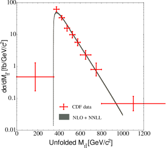
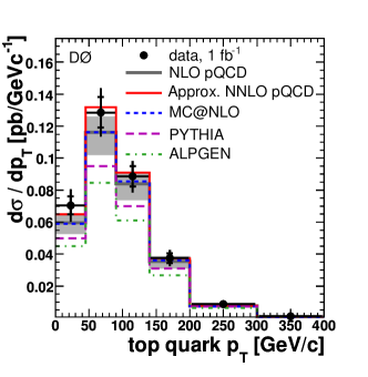
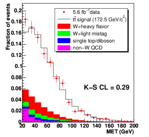
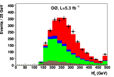
The measurements described in this Review use up to 5.8 fb^-1 of $p\bar{p}$ collision data. This corresponds to about $4\times 10^{4}$ $t\bar{t}$ events produced at each detector site. The size of this dataset allows for a thorough validation of the signal kinematics and acceptance modeling. Measurements of the inclusive $t\bar{t}$ cross section [24, 68, 85, 86, 87, 88, 89] indicate that applying an NLO-to-LO K-factor to the PYTHIA/ALPGEN simulations results in a very good agreement between predicted and observed rates of the $t\bar{t}$ signal and background processes. Measurements of $t\bar{t}$ differential cross sections [30, 31] attest to the correctness of recent Monte Carlo predictions which incorporate NLO and approximate NNLO computations, as illustrated in Figure 14. Consistency between observations and Monte Carlo predictions has been verified for a large number of experimental distributions, with two examples provided in Figure 15.

Figure 14: Example tests of the top quark pair production modeling at CDF and DØ. The left plot shows the differential $\sigma_{t\bar{t}}$ as a function of the invariant mass of the $t\bar{t}$ system, together with the approximate NNLO SM predictions [30, 200]. The plot on the right shows the ratio between data and NLO theoretical prediction of the distribution of the top quark $p_{T}$, together with approximate NNLO predictions and expectations from several Monte Carlo generators [31].

Figure 15: Distribution of the ${\not}{E_{T}}$ (left plot) modeled in the CDF top mass measurement [90] and $\mathrm{H_{T}^{l}}$ (right plot) in top-antitop events in the $\ell$+jets final state in the DØ  top cross section measurement. The $\mathrm{H_{T}^{l}}$ variable is defined as the scalar sum of the transverse energies of the jets and of the charged lepton [68].

4.2 Modeling of the physics backgrounds

The CDF and DØ  collaborations employ several Monte Carlo generators to model $t\bar{t}$ backgrounds processes. Both collaboration use ALPGEN for simulating $W$+jets production, with parton showering and hadronization performed by PYTHIA. The event samples are generated with the renormalization and factorization scale, $Q^{2}$, set to $M_{\mbox{\scriptsize\,W}}^{2}+\sum_{partons}p_{T}^{2}$. The overall normalization of the $W$+jets background is obtained from data by subtracting other physics and instrumental backgrounds and the $t\bar{t}$ signal as a function of jet multiplicity. The $W$+jets background is subdivided into three exclusive categories according to the flavor of the partons produced in association with the $W$ boson: (i) $W+b\bar{b}/c\bar{c}$ is the agglomeration of all final states which include the $W$ boson, the $b\bar{b}$ or $c\bar{c}$ quark pair, and any number of additional jets; (ii) $W+c$ consists of events with a $W$ boson produced with a single charm quark and any number of additional jets; and (iii) events in which the $W$ bosons are produced together with light flavor jets. The relative contributions from these three classes of events are determined using NLO QCD calculations based on the MCFM generator [91].

The diboson processes ($WW$, $WZ$, $ZZ$) are simulated using PYTHIA. Single top quark $s$- and $t$-channel production is simulated with COMPHEP [92] for DØ  measurements, and with MadEvent [76] for CDF measurements. The contributions from these background sources are normalized to the corresponding NLO predictions.

QCD multijet production is the major background to $t\bar{t}\to q_{1}\bar{q}_{2}bq_{3}\bar{q}_{4}\bar{b}$. The production of six or more partons is poorly understood at the theoretical level. In addition, the large multijet production cross section combined with the powerful background rejection needed to isolate the all-hadronic $t\bar{t}$ signal translates into a computationally prohibitive demand to generate an enormous number of events. For the above reasons, the multijet background is modeled using data in a region depleted of $t\bar{t}$ signal. Application of $b$-tagging techniques is necessary in the all-hadronic channel to achieve a reasonable S/B ratio. CDF uses collisions with at least six jets in the final state to model the QCD background, and corrects for the bias introduced by $b$-tagging using a parametrization of the $b$-tag rate derived with an independent dataset devoid of QCD events. The validity of this model is tested in large-statistics control samples deprived of top-antitop events.

5 Data analysis techniques

In this section we utilize the following notation. The symbol ${\bf x}$ is used to denote the collection of parton-level kinematic quantities needed in order to completely define an inelastic hard scattering reaction at the leading order perturbation theory (i.e., to specify a point in the reaction phase space). In all data analysis methods described, it is always assumed that points ${\bf x}$ in different collisions are independent and identically distributed (i.i.d.). The symbol ${\bf y}$ refers to one or more “observed” quantities inferred from detector data on event-by-event basis. Both the probabilistic nature of ${\bf x}$ and the nondeterministic detector response contribute to the randomness of ${\bf y}$. Even though we call ${\bf y}$ an “observed” quantity, it is usually a product of a sophisticated event reconstruction procedure which involves pattern recognition, tracking, clustering of jets, kinematic fitting, etc. It is commonly assumed that values of ${\bf y}$ are also i.i.d., and efforts are made to ensure effective i.i.d. behavior if this is not the case.

5.1 Major issues for different $t\bar{t}$ topologies

In the process of analyzing collision data for the purpose of measuring M${}_{\mbox{\scriptsize\,t}}$, several important decisions have to be made about statistical and computational techniques applied, signal and background modeling, measurement calibration, trade-off between expected statistical and systematics uncertainties, etc. Different techniques adopted by different authors resulted in a variety of substantially distinct data analysis approaches, with both complementary and competing features. In each approach, the following major issues have to be considered and addressed in a consistent manner:

• Choice of the $t\bar{t}$ final state. The traditional taxonomy of dilepton, $\ell$+jets and all-hadronic final states dictated by distinct event kinematics and different levels of background contamination is maintained by most authors, although joint measurements which combine events with different final states started to appear in the literature [93, 94, 65]. The main advantage of such joint measurements is the ability to apply the detector jet energy scale calibration obtained in the final states with hadronic $W$ decays to the dilepton channel.

• Event sample selection. Less strict event selection criteria can result in improved statistical uncertainty at the cost of increased background fraction and more complicated calibration.

• Degree to which the method depends on the calibration of the detector jet energy scale — the largest source of systematic uncertainty in the most precise CDF and DØ  measurements of M${}_{\mbox{\scriptsize\,t}}$.

• Level of detail in the statistical model of detector response to jets (for methods which do rely on jet energy reconstruction).

• Mapping of the objects reconstructed in the detector to the leading order parton-level entities. The difficulty here is due to the fact that the charge and the flavor of jets produced in top decays and associated processes (e.g., initial and final state QCD radiation) can not be measured with certainty. This leads not only to the ambiguity of assigning jets to the $t\bar{t}$ decay products but also to the problem of choosing a correct set of jets when the number of jets observed exceeds the number of strongly interacting partons produced in the leading order perturbation theory. In the $\ell$+jets and dilepton channels, additional ambiguities arise when multiple solutions of kinematic equations for the $\nu$ momenta exist. In the top mass measurement literature, multiple acceptable mappings between partons and detected objects are called “permutations”.

The feasibility of a simple kinematical analysis of the $p\bar{p}\rightarrow t\bar{t}\rightarrow W^{+}bW^{-}\bar{b}$ process can be determined using the following considerations. Charged leptons in decays of $W$ bosons are produced in association with neutrinos. Lepton presence, while allowing for powerful discrimination of QCD background, leads to complications in the reconstruction of event kinematics due to undetected neutrinos. We assume for the moment that the four-momenta of all charged final state partons are reasonably well measured, that masses of initial state partons and final state neutrinos are zero, that the transverse momentum of the incoming partons is zero, and that all of the event transverse missing energy is taken away by escaping neutrinos. With these assumptions, the neutrino 3-momenta and the longitudinal components of the momentum of the incoming partons are the only kinematical quantities not known, and then the total number of additional kinematic constraints needed in order to completely specify the reaction is $2+3n_{\nu}$, where $n_{\nu}$ is the number of neutrinos in the final state. Four of these constraints come from the energy-momentum conservation, and three additional constraints can be introduced by using the narrow width approximation for top and $W$: the invariant masses of the $W$ decay products are required to be consistent with the mass of the $W$ and the invariant masses of top decay products are set to M${}_{\mbox{\scriptsize\,t}}$. M${}_{\mbox{\scriptsize\,t}}$ itself is considered unknown, so the latter requirement generates only one effective constraint for the two top quarks present in the process. With these seven constraints, the total number of kinematical degrees of freedom (DoF) is $3n_{\nu}-5$. This gives 1 DoF for the dilepton final state, $-2$ for $\ell$+jets (the system is overconstrained), and $-5$ for the all-hadronic channel. This indicates that kinematic fitting techniques based on $\chi^{2}$ minimization can be utilized for the analysis of both $\ell$+jets and all-hadronic final states. In the dilepton channel kinematical equations are underconstrained, so this channel has to be treated in a substantially different manner. Kinematical analysis of $t\bar{t}$ events in different final states is described in more detail in Section 5.3.

From the statistical point of view, the result of any M${}_{\mbox{\scriptsize\,t}}$ measurement is an interval estimate of this parameter. Most authors utilize frequentist confidence intervals [95] by numerically studying the distribution of the point estimator with Monte Carlo simulations. Use of Bayesian credible intervals for top mass estimation has also appeared in the literature [96, 97, 98, 99]. Techniques used for constructing the point estimator itself are described in detail in the remainder of this section.

5.2 Methods based on distribution fitting

An unbiased point estimator of M${}_{\mbox{\scriptsize\,t}}$ can be obtained by fitting a distribution of some observed quantity ${\bf y}$ to a sum of signal and background contributions. In principle, any quantity whose distribution depends on the parameter of interest can be used to build an estimate of that parameter. In practice, one strives to choose ${\bf y}$ satisfying the following conditions:

• The sensitivity of the combined (signal plus background) distribution of ${\bf y}$ to M${}_{\mbox{\scriptsize\,t}}$ is high. A quantitative measure of such a sensitivity can be provided, for example, by Fisher information [95]. All other factors being equal, a measurement which uses a distribution with higher sensitivity to M${}_{\mbox{\scriptsize\,t}}$ will have lower statistical uncertainty.

• Modification of distribution nuisance parameters, such as detector calibration constants and sample signal fraction, does not lead to a noticeable change of the M${}_{\mbox{\scriptsize\,t}}$ estimate (i.e., off-diagonal elements of the Fisher information matrix which involve M${}_{\mbox{\scriptsize\,t}}$ should be small).

It can be easily appreciated that, in the case of M${}_{\mbox{\scriptsize\,t}}$ measurements at CDF and DØ, these conditions are contradictory. For example, an M${}_{\mbox{\scriptsize\,t}}$ estimate with high sensitivity can be obtained by calculating the invariant mass of three jets produced in the decay $t\rightarrow Wb\rightarrow jjb$ (assuming for the moment that the jets can be chosen correctly). This invariant mass is proportional to the detector jet energy scale with coefficient of proportionality close to unity. As discussed in Section 3.3, a few percent relative uncertainty is typical for standard jet energy scale calibrations. This uncertainty immediately translates into a strong limitation on the precision of the M${}_{\mbox{\scriptsize\,t}}$ determination in such a measurement.

For any particular M${}_{\mbox{\scriptsize\,t}}$ measurement technique, the relative contributions of statistical and systematic uncertainties vary with the amount of available data. To first order, the statistical uncertainty is expected to scale in proportion to $1/\sqrt{\int\mathcal{L}dt}$. Due to improvements in detector calibration and Monte Carlo simulations, the systematic uncertainty also decreases as $\int\mathcal{L}dt$ increases, albeit at a slower rate. Combined with the rich set of possible ${\bf y}$ choices, this variability resulted, over time, in a large number of studies which use distribution fitting for the M${}_{\mbox{\scriptsize\,t}}$ determination. Both signal and background distributions of ${\bf y}$ are constructed from Monte Carlo samples, for a set of discrete values of M${}_{\mbox{\scriptsize\,t}}$. Recent works also include the jet energy scale as the second parameter, so that the set of distributions is initially defined on a 2-d parameter grid. These Monte Carlo-derived distributions are called “templates”, and the whole technique of distribution fitting is referred to as “the template method” in the top mass measurement literature. The following ${\bf y}$ quantities have been utilized:

• Event-by-event top mass estimates $m_{t}$. Due to its relative simplicity and adequate sensitivity, this is by far the most popular approach [100, 101, 102, 103, 104, 105, 106, 107, 108, 109, 110, 111, 112, 87, 113]. Kinematical techniques used to obtain these estimates are presented in Section 5.3. An example set of $m_{t}$ templates is shown in Figure 16, taken from [114].

  

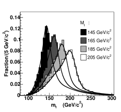
  Figure 16: Reconstructed $m_{t}$ distributions from simulated $p\bar{p}\rightarrow t\bar{t}$ events, for several different M${}_{\mbox{\scriptsize\,t}}$ values. Events in the samples used to build these templates have exactly one $b$-tagged jet. The overlayed curves are continuous template parameterizations [114].

• The transverse mass $m$${}_{\mbox{\scriptsize\,T2}}$ [115]. This kinematic variable approximates $m_{t}$ in a manner appropriate for use with two missing neutrinos in the dilepton final state.

• Combination of $m_{t}$ and $W$ mass [116, 114, 117, 93]. The $W$ mass is included in order to decrease the sensitivity to changes in the jet energy scale. Two $m_{t}$ values (which correspond to the best and second best jet-to-parton assignment) are used in [65, 118] which results in a 3-dimensional template.

• $m_{t}$ and the scalar sum of the $p_{T}$ of the four leading jets [119].

• $m_{t}$ and $H_{T}$ [93].

• $m_{t}$ and $m$${}_{\mbox{\scriptsize\,T2}}$ [65].

• $m_{t}$ and its estimated resolution, $\sigma$ [112, 66].

• Invariant mass of the charged lepton and the $b$ quark or energy of the two highest $E_{T}$ jets (early dilepton channel measurement [120]).

Several template techniques have been developed with the explicit goal of minimizing the dependence of the M${}_{\mbox{\scriptsize\,t}}$ estimate on the calorimeter jet energy scale. These techniques rely on the tracking information alone which eliminates the jet-related systematic uncertainty but also results in a substantial degradation of the measurement sensitivity. The following quantities have been employed for this purpose:

• The transverse decay length of $b$-tagged jets, L${}_{\mbox{\scriptsize\,xy}}$ [121, 122]. Average L${}_{\mbox{\scriptsize\,xy}}$ is increased with M${}_{\mbox{\scriptsize\,t}}$ because $b$ jets receive stronger transverse boost from heavier top quarks.

• The transverse momentum of leptons ($e$ and $\mu$) from $W$ decays [123, 122, 124, 125]. Example distributions of this and the previous quantity are shown in Figure 17.

  

  

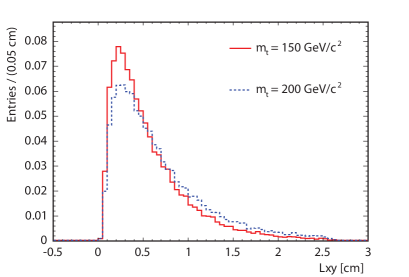
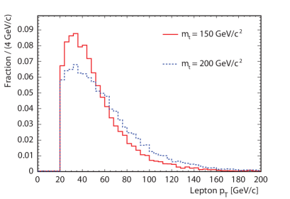
  Figure 17: The transverse decay length of $b$-tagged jets (left) and the transverse lepton momentum (right) for two different values of M${}_{\mbox{\scriptsize\,t}}$ separated by 50 GeV/c² [122].

• The invariant mass of the charged lepton from the $W$ decay and the muon from the semileptonic decay of the $b$ quark [126].

A number of measurements of the top quark mass in the dilepton channel by the DØ collaboration [127, 128, 110] utilized a unique template approach which does not quite fit in any of the categories already described. In this approach, weights are assigned to all $m_{t}$ values in each event according to the $\nu$WT algorithm (see Section 5.3 for the description of this procedure). In this algorithm, the $t{\bar{t}}$ production and decay processes are not modeled in sufficient detail and background contamination is not accounted for, so in practice the weights can not be treated as $m_{t}$ likelihoods. Instead, a method has been developed in which the probability of the complete $m_{t}$ weight distribution is estimated for each event as a function of M${}_{\mbox{\scriptsize\,t}}$. For the purpose of dimensionality reduction, the normalized weight curve is split into $N_{b}$ bins, weights are integrated in each bin, and the ($N_{b}-1$)-dimensional vector of integrated weights is used as ${\bf y}$ (due to the imposed normalization, $N_{b}-1$ weights are independent). According to [127], this approach improves the statistical sensitivity of the measurement by $\approx$25% in comparison with $m_{t}$ templates.

For any choice of ${\bf y}$, initial template construction is performed by nonparametric density estimation techniques. Simple histogramming is sufficient in case ${\bf y}$ is one-dimensional, while multivariate templates are usually built by kernel density estimation [129]. Fitting of the template distributions to the observed data is performed by the maximum likelihood method, with MINUIT [130] being the common choice of the optimization and error analysis engine. To ensure proper fit convergence, it is highly desirable for the likelihood to have at least two continuous derivatives as a function of each parameter. However, Monte Carlo-derived templates are only defined for a discrete parameter set. Two distinct solutions to this problem have been identified:

• A continuous parametric statistical model is fitted to the templates so that they become continuous functions, together with their first few derivatives, of both their parameters and ${\bf y}$. In this approach, the likelihood for the data can be determined for arbitrary parameter values, and it is continuous.

• The log-likelihood is initially determined for the parameter values for which templates were defined. Then the log-likelihood itself is interpolated to other parameter values using, for example, local polynomial regression [131], or by simply fitting the log-likelihood to a second or third degree polynomial near the peak. The smoothness assumptions are thus introduced directly into the likelihood curve.

The second solution is also widely employed by the phase space integration methods described in Section 5.4. There, direct calculation of the likelihood for arbitrary parameter values becomes too expensive CPU-wise, so one has to resort to interpolation.

Let’s assume that a continuous representation of the signal and background templates, $S({\bf y}|M_{\mbox{\scriptsize t}},{\bf\theta})$ and $B({\bf y}|M_{\mbox{\scriptsize t}},{\bf\theta})$, respectively, is available. Here, ${\bf\theta}$ represents nuisance parameters of the measurement other than the sample signal fraction (typically, jet energy scale). Then a simple likelihood for the observed sample can be written as

$$\begin{array}[]{ll}L(M_{\mbox{\scriptsize t}},{\bf\theta},f_{s})=\prod_{j=1}^{N}&{\!\!\!\!\!}\left[f_{s\,}S({\bf y}_{j}|M_{\mbox{\scriptsize t}},{\bf\theta})\right.\\ &{\!\!\!\!\!}\left.+\,(1-f_{s})B({\bf y}_{j}|M_{\mbox{\scriptsize t}},{\bf\theta})\right],\\ \end{array}$$ (1)

where $j=1,2,...,N$ is the event number in the sample and $f_{s}$ is the sample signal fraction. The subsequent elimination of the nuisance parameters ${\bf\theta}$ and $f_{s}$ is performed either by profiling or by marginalization. The profiling procedure consists in maximizing the likelihood (1) with respect to ${\bf\theta}$ and $f_{s}$ for each value of M${}_{\mbox{\scriptsize\,t}}$. Marginal likelihood is instead calculated by introducing a prior distribution for the nuisance parameters (such a prior distribution usually takes into account uncertainties of existing estimates of these parameters) and integrating the likelihood over ${\bf\theta}$ and $f_{s}$ with the prior. Mixed treatments have been utilized as well, in which the likelihood is initially profiled over $f_{s}$ and then ${\bf\theta}$ is marginalized. Relative merits of likelihood profiling and marginalization are discussed, for example, in [132].

Various modifications of the basic likelihood (1) have been employed in a number of M${}_{\mbox{\scriptsize\,t}}$ measurements. These modifications take into account uncertainties in the $S({\bf y}|M_{\mbox{\scriptsize t}},{\bf\theta})$ and $B({\bf y}|M_{\mbox{\scriptsize t}},{\bf\theta})$ shapes due to the limited number of Monte Carlo events available [103, 107] as well as binning effects in case histogramming is used to build the templates [104, 133]. In addition, the observed event sample is often split into several non-overlapping subgroups (which differ, e.g., by the number of $b$-tagged jets) with different template shapes and expected background fractions. This allows for more precise template modeling in each subgroup as well as for the introduction of separate $f_{s}$ priors. After elimination of the nuisance parameters by profiling or marginalization, the M${}_{\mbox{\scriptsize\,t}}$ log-likelihoods from different subgroups are added together to obtain the final result.

The “ideogram” technique is a modification of the template method which attempts to take into account the resolution of the $m_{t}$ estimate on event-by-event basis [59, 134, 135, 136]. All M${}_{\mbox{\scriptsize\,t}}$ measurements which utilized this technique so far lacked a consistent likelihood formulation owing to the absence of the resolution prior, as discussed in detail in [137]. Perhaps, this is the reason why such measurements did not demonstrate convincing uncertainty improvements over results obtained with templates.

The top quark mass can also be estimated indirectly from the measurement of the $t{\bar{t}}$ production cross section [138, 111, 139], assuming that the cross section dependence on M${}_{\mbox{\scriptsize\,t}}$ can be determined with sufficient precision from the Standard Model theoretical calculations.

5.3 Kinematic reconstruction of the top mass

In the $\ell$+jets and all-hadronic channels the number of available kinematic constraints exceeds the number of unknown quantities (including M${}_{\mbox{\scriptsize\,t}}$ itself), therefore these channels are amenable to kinematic fitting using $\chi^{2}$ minimization. The $\chi^{2}$ is constructed using transverse momenta of detected leptons and jets as well as the missing transverse energy:

$$\begin{array}[]{rl}\chi^{2}=&\sum_{i=\ell,4jets}\frac{(p_{T}^{i,fit}-p_{T}^{i,meas})^{2}}{\sigma_{i}^{2}}\\ &+\sum_{j=x,y}\frac{(p_{j}^{UE,fit}-p_{j}^{UE,meas})^{2}}{\sigma_{UE}^{2}}\\ &+\,\frac{(M_{\ell\nu}-M_{W})^{2}}{\Gamma_{W}^{2}}+\frac{(M_{jj}-M_{W})^{2}}{\Gamma_{W}^{2}}\\ &+\,\frac{(M_{b\ell\nu}-m_{t})^{2}}{\Gamma_{t}^{2}}+\frac{(M_{bjj}-m_{t})^{2}}{\Gamma_{t}^{2}}.\end{array}$$ (2)

This particular expression is appropriate for the $\ell$+jets channel (the notation follows [114]). Symbols with superscript fit denote fitted parton-level variables which determine leading order $t\bar{t}$ production and decay kinematics, while superscript meas refers to quantities measured in the detector. The quantities used to form this expression are:

• $p_{T}^{i}$ are transverse momenta of leptons and quarks (fitted) or jets (measured).

• $p_{j}^{UE}$ are the transverse components of the unclustered energy. The transverse momenta of the jets, neutrino, and unclustered energy are related at the parton level by ${\vec{p}}_{T}^{\,\nu}=-\left({\vec{p}}_{T}^{\,\ell}+\sum{\vec{p}}_{T}^{\,jet}+{\vec{p}}_{T}^{\,UE}\right)$, assuming that the initial transverse momentum of the colliding particles is ${\vec{0}}$.

• $M_{\ell\nu}$, $M_{jj}$ are invariant masses of $W$ decay products constructed using parton-level quantities.

• $M_{b\ell\nu}$, $M_{bjj}$ are invariant masses of top quark decay products constructed using parton-level quantities.

The $\chi^{2}$ for the all-hadronic channel is similar, with light jets used everywhere instead of $\ell$ and $\nu$, the first sum running over 6 jets, and the $p_{j}^{UE}$ terms omitted [87, 105].

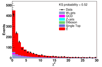
In (2), Gaussian resolution functions are employed for magnitudes of all transverse momenta, missing energy, as well as for the mass constraints. The method does not take into account angular resolutions of lepton and jet directions (these directions are assumed to be perfectly measured), asymmetry of jet $p_{T}$ resolution functions, or expected event population in the reaction phase space. The $\chi^{2}$ is minimized with respect to all parton-level kinematic quantities (magnitudes of the transverse momenta of $b$ and light quarks, 3-momentum of the neutrino) as well as $m_{t}$. This minimization is performed separately for all jet-to-parton assignments (permutations) consistent with the observed set of $b$ tags. Typically, two solutions are obtained in the $\ell$+jets channel when kinematic equations are solved for the $t\rightarrow Wb\rightarrow\ell\nu_{\ell}b$ decay sequence, thus increasing the number of effective permutations by a factor of two. The value of $m_{t}$ at the $\chi^{2}$ minimum over all permutations and parton-level kinematic variables is usually taken as the top mass estimate for the event. Distributions of the $\chi^{2}$ minimum values are illustrated in Figure 18 for the $\ell$+jets channel.

Figure 18: Minimum $\chi^{2}$ distribution for events with at least one $b$ tag in the CDF 5.6 fb${}^{\mbox{\scriptsize-1}}$ event sample [65].

Several modifications of this basic approach were explored, typically resulting in a more complicated method with only a slight improvement in the measurement sensitivity:

• Use of $m_{t}$ estimates from more than one permutation [104, 140, 65].

• Inclusion of the jet angular resolution terms [101, 104, 103, 119].

• Use of a separate jet energy scale factor for each permutation [119].

• Addition of a term which models the $b$ tagging probability [103].

• Replacement of Gaussian mass constraints with Breit-Wigner constraints [104].

Another possible modification that has not been tested yet in the context of M${}_{\mbox{\scriptsize\,t}}$ measurements consists in replacing the mass constraints in (2) with the term $-2\ln[\,p({\bf x}|m_{t})\,J^{-1}\,p_{tag}]$, where $p({\bf x}|{\it M}_{\mbox{\scriptsize\,t}})$ represents the phase space density of the process normalized by the total observable cross section, $J=\left|\frac{\partial\,{\bf p}^{fit}}{\partial\,{\bf x}}\right|$ is the Jacobian which relates the fitted quantities as well as the quantities which are assumed to be perfectly measured to the phase space variables, and $p_{tag}$ is the permutation-specific probability of the observed $b$ tag configuration (see Section 5.4). The goal is to find the most probable values of all fitted quantities taking into account theoretical assumptions about the reaction and thereby to profile the $m_{t}$ likelihood over the complete parton-level phase space.

For the dilepton channel, the number of constraints is insufficient to determine $m_{t}$. It would be possible to infer $m_{t}$ if at least one additional kinematic quantity or constraint was available. This suggests the following method of $m_{t}$ determination: values of some unobserved kinematic quantities $\xi$ are assumed, kinematic equations are solved, and allowed values of top mass, $m_{t}^{\prime}(\xi,{\bf y})$, are determined (in addition to $\xi$, $m_{t}^{\prime}(\xi,{\bf y})$ depends on some or all quantities ${\bf y}$ measured in the detector). $\xi$ values are scanned within their kinematic limits. Obtained $m_{t}^{\prime}(\xi,{\bf y})$ values are assigned weights proportional to the probability density, $\rho(\zeta)$, of some other kinematic quantities $\zeta(\xi,{\bf y})$ (variable sets $\xi$ and $\zeta$ may overlap partially, completely, or not at all). $\rho(\zeta)$ is determined in advance, either from theoretical considerations or by estimating this density numerically using large samples of Monte Carlo events. While it is not strictly necessary, this method operates in the most transparent manner if $\rho(\zeta)$ has little or no dependence on M${}_{\mbox{\scriptsize\,t}}$. The distribution of possible $m_{t}$ values, $\rho(m_{t})$, is thus formed, proportional to $\int\rho(\zeta(\xi,{\bf y}))\,\delta(m_{t}^{\prime}(\xi,{\bf y})-m_{t})\,d\xi$. The location parameter of this distribution (usually the mode) is used as the top mass estimate for this particular event. This approach is very general, and a judicious choice of $\xi$ and $\zeta$ variables will produce an estimate with good sensitivity to M${}_{\mbox{\scriptsize\,t}}$ while maintaining a relatively simple statistical model for $\rho(\zeta)$ (inclusion of all parton-level phase space variables in both $\xi$ and $\zeta$ leads to techniques described in Section 5.4).

The following choices of $\xi$ and $\zeta$ have been explored:

• $\xi=(\eta_{\nu},\eta_{\bar{\nu}})$: a two-dimensional variable, where $\eta_{\nu}$ and $\eta_{\,\bar{\nu}}$ are pseudorapidities of the neutrinos. $\zeta=(\eta_{\nu},\eta_{\bar{\nu}},{\not}{\vec{E}_{T}})$, where ${\not}{\vec{E}_{T}}$ is the two-dimensional missing transverse energy. This method is called neutrino weighting algorithm ($\nu$WT) [128, 102, 107, 110, 112, 66, 65, 142]. Weight distributions for the six dilepton events from [128] are shown in Figure 19.

  

  Figure 19: Weights for the individual events in the DØ Run I dilepton $\nu$WT analysis as a function of $m_{t}$ [128].

• $\xi=(\varphi_{\nu},\varphi_{\bar{\nu}})$, where $\varphi_{\nu}$ and $\varphi_{\bar{\nu}}$ are neutrino azimuthal angles in the plane transverse to the beam. A $\chi^{2}$ variable formed in a manner similar to (2) is utilized as $\zeta$ (since values of two variables are assumed, the number of constraints exceeds the number of unknowns by 1, so it becomes possible to construct a meaningful $\chi^{2}$). Weights proportional to $e^{-\chi^{2}/2}$ are assigned to $m_{t}(\xi,{\bf y})$ solutions. This method is referred to as the neutrino $\varphi$ weighting algorithm (PHI) [107, 108].

• $\xi=(m_{t}^{\prime},p_{\ell^{+}},p_{\ell^{-}},p_{b},p_{\,\bar{b}})$, $\zeta={\bf x}$, where ${\bf x}$ represents all leading order parton-level variables which determine the reaction kinematics. Directions of the charged leptons and $b$ quarks are assumed to be perfectly measured, while magnitudes of their momenta (inverse magnitude in the case of $\mu$) are varied within their expected Gaussian resolutions. Neutrino momenta are calculated from kinematic constraints in the narrow width approximation for $t$ and $W$ and zero transverse momentum assumption for the $t\bar{t}$ system. Values of $m_{t}=m_{t}^{\prime}$ are weighted by the phase space density of the process at ${\bf x}$, summed over all possible kinematical solutions for the neutrinos and jet-to-quark assignments. This approach is known as the matrix element weighting algorithm (${\mathcal{M}}$WT) [143, 128, 110, 112]. It is a direct precursor of the phase space integration methods described in Section 5.4.

• $\xi=\zeta=(p_{z}^{t\bar{t}},E_{b},E_{\bar{b}},{\not\!E}_{T})$, where $p_{z}^{t\bar{t}}$ is the z component (along the beam) of the $t\bar{t}$ system, while $E_{b}$ and $E_{\bar{b}}$ are the energies of the $b$ and $\bar{b}$ quarks, respectively. The probability density of $\zeta$ is factorized into the product of probabilities for individual components, with all marginals represented by Gaussian distributions and correlations neglected. This method is known as the full kinematic analysis (KIN) [107].

It appears that the M${}_{\mbox{\scriptsize\,t}}$ sensitivity of the ${\mathcal{M}}$WT and $\nu$WT algorithms is similar [112] and slightly exceeds that of both PHI and KIN methods [107]. In order to increase the overall sensitivity, results obtained in the dilepton channel on the same data with multiple template methods are often combined using the “best linear unbiased estimator” (BLUE) approach [144, 145]. In this case correlation coefficients between different methods are determined using common pseudo-experiments.

5.4 Phase space integration methods

The technique of calculating event observation probabilities by integrating over all parton-level quantities in the reaction phase space was introduced into the high energy physics data analysis practice in the pioneering Run I measurement of the top quark mass by the DØ collaboration [96]. This method can be understood as an application of the Bayesian principle of integrating over all unobserved degrees of freedom with a well-motivated informative prior provided by the Standard Model theory (i.e., event-by-event marginalization of ${\bf x}$). The prior is proportional to the matrix element squared of the process, so the technique is often referred to as the “matrix element method” (MEM). The probability of observing quantities ${\bf y}$ in a particle detector, $P_{\mbox{\scriptsize\,ev}}({\bf y}|{\bf a})$, is determined according to

$$P_{\mbox{\scriptsize\,ev}}({\bf y}|{\bf a})=\sum_{i}f_{i}P_{i}({\bf y}|{\bf a}),$$ (3)

where ${\bf a}$ is the set of model parameters. This set includes M${}_{\mbox{\scriptsize\,t}}$ and can also include detector jet energy scale as well as other theoretical and instrumental quantities. $f_{i}$ are the fractions of different non-interfering production channels consistent with ${\bf y}$ and constrained by $\sum_{i}f_{i}=1$. In the context of M${}_{\mbox{\scriptsize\,t}}$ measurements, the probability to measure ${\bf y}$ in each channel $i$ is most often estimated from

$$\begin{array}[]{ll}P_{i}({\bf y}|{\bf a})=&{\!\!\!\!\!}\frac{\Omega({\bf y})}{\sigma_{i}({\bf a})A_{i}({\bf a})}\\ &{\!\!\!\!\!}\times\int_{\Phi_{i}}W_{i}({\bf y}|{\bf x},{\bf a})\,|M_{i}({\bf x},{\bf a})|^{2}\,T_{i}({\bf x},{\bf a})\,d{\bf x},\end{array}$$ (4)

where the following notation is utilized:

$\Omega({\bf y})$ — Indicator function for the analysis acceptance (1 for events which pass the event selection criteria, 0 otherwise). This term can be replaced by 1 in case only accepted events are considered.

${\bf x}$ — Variables which uniquely specify a point in the channel phase space $\Phi_{i}$, ${\bf x}\in\Phi_{i}$.

$d{\bf x}$ — Differential element of the phase space $\Phi_{i}$.

$\sigma_{i}({\bf a})$ — Channel cross section:

$$\sigma_{i}({\bf a})=\int_{\Phi_{i}}|M_{i}({\bf x},{\bf a})|^{2}\,T_{i}({\bf x},{\bf a})\,d{\bf x}.$$

$A_{i}({\bf a})$ — Overall experimental acceptance for channel $i$.

$W_{i}({\bf y}|{\bf x},{\bf a})$ — Detector transfer function (TF). This is the probability density for observing detector response ${\bf y}$ from the space of possible measurements $Y$ when the “true” phase space coordinate of the event is ${\bf x}$. This function should be normalized for every value of $i$, ${\bf x}$, and ${\bf a}$ either by $\int_{Y}W_{i}({\bf y}|{\bf x},{\bf a})\,d{\bf y}=1$ or by $\int_{Y}\Omega({\bf y})W_{i}({\bf y}|{\bf x},{\bf a})\,d{\bf y}=\epsilon_{i}({\bf x},{\bf a})$, where $\epsilon_{i}({\bf x},{\bf a})$ is the efficiency to detect an event with phase space coordinate ${\bf x}$. The difference between these TF normalization conditions and their effect on TF modeling is discussed in [146].

$|M_{i}({\bf x},{\bf a})|^{2}$ — Squared matrix element of the process.

$T_{i}({\bf x},{\bf a})$ — Other factors which do not depend on ${\bf y}$ (e.g., flux of colliding beams, parton distribution functions).

In a compact symbolic notation, (4) can be represented as

$$P_{i}({\bf y}|{\bf a})=\frac{1}{\sigma_{i,obs}({\bf a})}\frac{d\sigma_{i,obs}({\bf y}|{\bf a})}{d{\bf y}},$$ (5)

where $\frac{d\sigma_{i,obs}({\bf y}|{\bf a})}{d{\bf y}}$ is the differential observable cross section for channel $i$. Parameter set ${\bf a}$ is estimated by maximizing the likelihood which is constructed by multiplying probabilities for all events in the sample: $L({\bf a})=\prod_{j=1}^{N}P_{\mbox{\scriptsize\,ev}}({\bf y}_{j}|{\bf a})$. The denominator term $\sigma_{i,obs}({\bf a})=\sigma_{i}({\bf a})A_{i}({\bf a})=\int_{Y}\frac{d\sigma_{i,obs}({\bf y}|{\bf a})}{d{\bf y}}d{{\bf y}}$ (total observable cross section) ensures proper likelihood normalization.

The MEM statistical model of a particle physics process is significantly more precise than the models employed by the distribution fitting methods, as it takes into account the process phase space density. Detailed shapes of detector transfer functions can be utilized, while techniques based on $\chi^{2}$ minimization essentially assume Gaussian resolutions. These and other advantages of MEM [146] result in an improved statistical precision of the parameter estimates. On the other hand, efficient calculation of the phase space integral (4) is nontrivial, as it can not be performed with standard phase space sampling schemes developed for Monte Carlo event generation because of the presence of transfer functions which alter the peak structure of the integrand. This situation resulted in a development of a number of ad hoc dimensionality reduction and phase space sampling schemes for calculating (4) in the context of the $t\bar{t}$ production and decay. A recent study [147] attempts to address this problem in a systematic manner for a number of processes.

All M${}_{\mbox{\scriptsize\,t}}$ measurements performed so far integrate (4) over the leading order parton phase space, so that the final state “soft QCD” processes (parton showering and hadronization) are combined together with the detector response, and this combination is subsequently modeled empirically by the detector transfer function. For each channel, the transfer function of the process is factorized into a product of transfer functions for $K$ individual partons traced in the detector (neutrinos are excluded):

$$W({\bf y}|{\bf x},{\bf a})=\sum_{\pi[m_{1},...,m_{K}]}\prod_{k=1}^{K}p_{m_{k}k}W_{k}({\bf y}_{m_{k}}|{\bf x}_{k},{\bf a}),$$ (6)

where ${\bf x}_{k}$ is the phase space coordinate of the $k$${}^{\mbox{\scriptsize th}}$ parton, ${\bf y}_{m_{k}}$ are the measured quantities for the “physics object” with index $m_{k}$ (jet, lepton candidate) obtained in the event reconstruction and pattern recognition process, $p_{m_{k}k}$ are the prior probabilities for associating parton $k$ with physics object $m_{k}$, and the channel index $i$ is omitted for brevity. The sum is performed over $K!$ possible assignments of indices $[m_{1},...,m_{K}]$ to permutations of $[1,...,K]$. For $t\bar{t}$ signal modeling, it can be assumed that leptons are identified unambiguously (i.e., $p_{m_{k}k}$ is reduced to Kronecker $\delta_{qk}$ in case the lepton has the index $q$ in the list of physics objects), but jet charge and flavor can not be determined with complete certainty. A number of measurements [148, 149, 98, 99] utilized the following $p_{m_{k}k}$ assignment scheme:

$p_{m_{k}k}=p_{\mbox{\scriptsize\,tag}}({\bf y})$ if $k$ refers to a $b$ or $\bar{b}$ quark in the final state and $m_{k}$ refers to a $b$-tagged jet reconstructed in the detector. $p_{\mbox{\scriptsize\,tag}}({\bf y})$ is the probability to flavor tag a $b$ jet as a function of its reconstructed momentum and other measured quantities (such as the number of tracks).

$p_{m_{k}k}=1-p_{\mbox{\scriptsize\,tag}}({\bf y})$ if $k$ refers to a $b$ or $\bar{b}$ quark in the final state and $m_{k}$ refers to an untagged jet.

$p_{m_{k}k}=p_{\mbox{\scriptsize\,mistag}}({\bf y},f)$ if $k$ refers to a light ($f=u$, $d$, or $s$) or charm ($f=c$) quark in the final state and $m_{k}$ refers to a $b$-tagged jet. $p_{\mbox{\scriptsize\,mistag}}({\bf y},f)$ is the probability to mistag a jet originating from a quark with flavor $f\neq b$ as a $b$ jet.

$p_{m_{k}k}=1-p_{\mbox{\scriptsize\,mistag}}({\bf y},f)$ if $k$ refers to a light or charm quark in the final state and $m_{k}$ refers to an untagged jet.

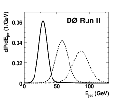
Although in practice the priors $p_{m_{k}k}$ are derived as functions of ${\bf y}_{m_{k}}$, their dependence on ${\bf y}$ is usually mild and can be neglected in comparison with the fast variation of $W_{k}({\bf y}|{\bf x}_{k},{\bf a})$. It is also commonly assumed that the overlap between phase space regions which contribute to different permutations is negligible. With these approximations, the transfer functions for individual partons can be normalized either by $\int_{Y_{k}}W_{k}({\bf y}_{k}|{\bf x}_{k},{\bf a})\,d{\bf y}_{k}=1$ or by $\int_{Y_{k}}\Omega_{k}({\bf y}_{k})W_{k}({\bf y}_{k}|{\bf x}_{k},{\bf a})\,d{\bf y}_{k}=\epsilon_{k}({\bf x}_{k},{\bf a})$. Both of these normalization conditions assume (either implicitly or explicitly) that the factorization model can also be applied to acceptance and efficiency. An example jet energy transfer function is shown in Figure 20.

Figure 20: Jet transfer functions for light quark jets, $|\eta|<0.5$, for parton energies $E_{p}=30$ GeV (solid curve), 60 GeV (dashed curve), and 90 GeV (dash-dotted curve). Perfect angular resolution is assumed [97].

Appropriate normalization for $p_{m_{k}k}$ depends, in general, on the precise meaning of these coefficients. For the flavor tagging scheme outlined above, it becomes $\sum p_{tag}=1$, where $p_{tag}=\prod_{k=1}^{K}p_{m_{k}k}$ is the permutation-specific probability of a certain heavy flavor tag assignment and the sum is performed over all $2^{K}$ possible assignments. Note the absence of the sum over permutations, contrary to the convention used by some authors [97]. Different permutations correspond to different phase space points, and the overall transfer function has to be normalized for each phase space point separately.

On top of the product model (6) for the detector transfer function, additional correction terms were utilized in a number of M${}_{\mbox{\scriptsize\,t}}$ measurements:

• Simplifying assumptions about jet transfer functions (e.g., perfect angular resolutions and independence of jet response from proximity to other jets) were partially compensated for either by adjusting the process phase space density (the “effective propagators” approach of [148]) or by introducing transfer functions which model smearing of the angular distances between jets [150].

• Presence of the initial state QCD radiation was modeled either with a prior on the transverse momentum of the $t\bar{t}$ system [148, 149, 151, 117] or with an explicit transfer function which takes into account additional energy visible in the detector and not associated with the $K$ most energetic physics objects expected at the leading order [152].

Out of the 32 variables needed to specify the phase space point for the $p\bar{p}\rightarrow t\bar{t}\rightarrow 6$ partons reaction, only the masses of initial partons and outgoing charged leptons and neutrinos can be considered exactly known. Taking into account the energy-momentum conservation, this leads to 22, 24, and 26-dimensional phase space integrals in the dilepton, $\ell$+jets, and all-hadronic channels, respectively. In case the integral (4) is evaluated by Monte Carlo integration, the relative precision of the result is $\delta_{rel}=(\sigma_{I}/\left<I\right>)\,N^{-1/2}$, where $\left<I\right>$ and $\sigma_{I}$ are, respectively, the average value and the standard deviation of the integrand, and $N$ is the number of integrand evaluations. $I$ is sharply peaked over small regions of phase space which leads to a large prefactor $\sigma_{I}/\left<I\right>$. For example, for the $W$ mass Breit-Wigner distribution integrated between 0 and M${}_{\mbox{\scriptsize\,t}}$, $\sigma_{I}/\left<I\right>\approx 3.5$, so that reaching relative precision of $10^{-3}$ requires $\sim 10^{7}$ integrand evaluations. Efficient Monte Carlo calculation of such integrals can be performed by applying convergence acceleration techniques, such as importance sampling and stratified sampling. These techniques, however, only work well if the peak structure of the integrand is factorizable in terms of integration variables. In (4), the peaks are not aligned with the momenta of final state particles in terms of which the phase space integration is formally defined. Instead, the transfer functions are concentrated around the observed directions of leptons and jets, while propagators in the matrix element are strongly peaked around $t$ and $W$ masses. Thus a change to a new, efficient variable set is necessary.

Another technique commonly used to make the prefactor smaller is dimensionality reduction: a constraint is imposed on the integration variables, and the integrand is evaluated only for the subspace defined by that constraint. A number of assumptions have been introduced by different authors for this purpose, in various combinations:

1. Assume that some or all of the quarks are on shell (i.e., masses of the light and $b$ jets are fixed). This assumption removes $n_{q}$ integration variables, where $n_{q}$ is the number of quarks in the final state.

2. Ignore individual transverse momenta of the incoming partons and consider only the transverse momentum of the $t\bar{t}$ system ($-2$ integration variables).

3. Assume that $t\bar{t}$ transverse momentum is 0 (this assumption is stronger than the previous one, $-4$ variables).

4. Assume that jet directions are perfectly measured in the detector. In this case, jet transfer functions are proportional to $\delta^{2}(\Omega-\Omega_{meas})$ ($-2\,n_{q}$ variables).

5. Assume that charged lepton momenta are perfectly measured ($-3\,n_{\ell}$ variables).

6. Use narrow width approximations for $t$ ($-2$ variables) and/or $W$ (also $-2$).

In principle, any such assumption reduces the fidelity of the statistical model, but practical considerations (in particular, the need to evaluate a large number of integrals for a set of parameter values using limited CPU resources) often take priority. For example, in the original MEM M${}_{\mbox{\scriptsize\,t}}$ measurement by DØ  in the $\ell$+jets channel [96], (i), (iii), (iv), and (v) were assumed which leads to a 5-d integral. Masses of $W$ and top resonances, as well as the momentum magnitude for one of the partons in the hadronic $W$ decay were chosen as integration variables. This resulted in a reasonably well factorized phase space peak structure, so the integrals could be subsequently evaluated automatically by the VEGAS [153] adaptive numerical integration program. In a recent $\ell$+jets M${}_{\mbox{\scriptsize\,t}}$ measurement by CDF [149], only (ii) and (v) were assumed which allowed the authors to employ detailed transfer function models and resulted in a 19-d integral. The convergence was accelerated by appropriate variable transformations (importance sampling), by early pruning of jet permutations with small contributions into the overall integral, and by use of low-discrepancy sequences [154] for points in which the integrand was evaluated (Quasi-Monte Carlo).

The Dynamical Likelihood Method (DLM) [155, 156] is a phase space integration technique which evaluates (4) in a particular manner. Note that the integral can be formally written as

$$\begin{array}[]{l}P_{i}({\bf y}|{\bf a})=\frac{\Omega({\bf y})}{\sigma_{i}({\bf a})A_{i}({\bf a})}\left<|M_{i}({\bf x},{\bf a})|^{2}\,T_{i}({\bf x},{\bf a})\right>_{G_{i}}\\ \times\int_{\Phi_{i}}W_{i}({\bf y}|{\bf x},{\bf a})d{\bf x},\end{array}$$ (7)

where $\left<...\right>_{G_{i}}$ stands for averaging over points ${\bf x}\in\Phi_{i}$ distributed in the phase space with density $G_{i}({\bf x}|{\bf y},{\bf a})\equiv\frac{W_{i}({\bf y}|{\bf x},{\bf a})}{\int_{\Phi_{i}}W_{i}({\bf y}|{\bf x},{\bf a})d{\bf x}}$. Following the naming convention of [156], we refer to $G_{i}({\bf x}|{\bf y},{\bf a})$ as posterior transfer function (PTF). Phase space sampling according to PTF efficiently takes into account all structure present in the integrand due to detector resolution (peaks in the matrix element still require special treatment). In principle, PTF can be derived from Monte Carlo simulations of the physics process and detector, using joint distributions of ${\bf x}$ and ${\bf y}$ in the region defined by $\Omega({\bf y})=1$, where every event enters with the weight $\left(|M_{i}({\bf x},{\bf a})|^{2}\,T_{i}({\bf x},{\bf a})\right)^{-1}$. In practice, however, due to large dimensionalities of ${\bf x}$ and ${\bf y}$, some kind of a PTF product model must be employed. When the terms in the PTF product expansion, such as jet posterior transfer functions, are derived, correlations between different ${\bf x}$ dimensions (caused, e.g., by energy-momentum conservation and complicated phase space boundaries) are ignored. During Monte Carlo integration, lepton and jet variables are sampled first, while proper kinematics is subsequently enforced by imposing constraints on invisible particles (neutrinos). In addition, the factor $\int_{\Phi_{i}}W_{i}({\bf y}|{\bf x},{\bf a})d{\bf x}$ which depends on ${\bf a}$ and normalizes $P_{i}({\bf y}|{\bf a})$ in (7) is usually neglected (i.e., assumed to be constant). Compounded, these approximations result in some degradation of the statistical model and a biased maximum likelihood estimator of M${}_{\mbox{\scriptsize\,t}}$ [157, 158, 159]. The estimator bias is subsequently removed by a calibration procedure (see Section 5.6).

5.5 Background handling

In addition to optimizing event sample selection requirements and heavy flavor tagging, a number of methods have been developed for the purpose of strengthening the background suppression and for taking into account background contamination in the M${}_{\mbox{\scriptsize\,t}}$ estimates. Increase in the signal fraction $f_{s}$ improves sample sensitivity to M${}_{\mbox{\scriptsize\,t}}$. At the same time, background discrimination should preferably be implemented in such a manner that this fraction (a nuisance parameter in the measurement) is not correlated strongly with the M${}_{\mbox{\scriptsize\,t}}$ estimate. The relative importance of these arguments in the context of any particular M${}_{\mbox{\scriptsize\,t}}$ measurement method is not obvious a priori. As the results (with the notable exceptions of [105, 160]) are usually presented without describing the extent to which different background suppression options were explored, relative merits of different background handling techniques are difficult to compare.

Correlation reduction between $f_{s}$ and M${}_{\mbox{\scriptsize\,t}}$ was emphasized in [101, 104]. With this purpose in mind, one can not rely upon the most distinguishing properties of $t\bar{t}$ events, the invariant masses of various jet combinations and the large amount of energy visible in the detector, for background rejection. Topological event characteristics have to be exploited instead, such as differences between angular distributions of $t\bar{t}$ decay products and particles produced in background processes. Even though there appears to be no simple kinematic variable of this kind with high discriminating power, optimized combinations of multiple variables have been used in practice with considerable success. For example, the “low bias discriminant” technique of [101, 104] developed for the $\ell$+jets channel employed a likelihood ratio discriminant in the form of a cut on D${}_{\mbox{\scriptsize\,LB}}({\bf y})=\frac{p_{s}({\bf y})}{p_{s}({\bf y})+p_{b}({\bf y})}$, where $p_{s}({\bf y})$ and $p_{b}({\bf y})$ are the quasi-probability densities of the signal and background, respectively. The set of observed variables y (missing transverse energy, aplanarity, centrality, and one other variable which characterizes average angular separation between jets) was chosen and the shapes $p_{s}({\bf y})$ and $p_{b}({\bf y})$ were tuned in such a manner that the distributions of D${}_{\mbox{\scriptsize\,LB}}({\bf y})$ were independent from M${}_{\mbox{\scriptsize\,t}}$. The discriminant distributions for simulated samples of signal and background events are shown in Figure 21.

Figure 21: The D${}_{\mbox{\scriptsize\,LB}}$ discriminant plotted for the ${\it M}_{\mbox{\scriptsize\,t}}=175$ GeV/$c^{2}$ $t\bar{t}$ sample (hatched) and the simulated background (not hatched). The histograms are normalized to the same area [104].

The D${}_{\mbox{\scriptsize\,LB}}({\bf y})$ cut was then optimized for the best overall statistical uncertainty while encumbering little correlation between $f_{s}$ and M${}_{\mbox{\scriptsize\,t}}$. The use of a neural network with the same input variables was explored as well, with similar results.

Neural networks have also found their use in the M${}_{\mbox{\scriptsize\,t}}$ measurements which do rely, at least partially, upon energy-dependent variables for background discrimination. According to this approach, better signal/background separation is valued over reduced correlation between $f_{s}$ and M${}_{\mbox{\scriptsize\,t}}$. These studies include [148, 149] in the $\ell$+jets channel and [106, 87, 105, 113] in the all-hadronic channel.

An advanced investigation of the effect of background suppression on the precision of M${}_{\mbox{\scriptsize\,t}}$ measurement in the dilepton channel has been carried out in [160]. In this study, a neural network with six input variables was directly optimized for the best statistical uncertainty of the M${}_{\mbox{\scriptsize\,t}}$ estimator. The estimator itself was obtained by MEM in which the background probability was calculated for the $Z/\gamma^{*}+2$ jets and $WW+2$ jets production as well as for jets faking leptons in $W+3$ jets. The NN optimization algorithm (neuroevolution) allowed for modification of both NN topology and weights. As a result, the space of potential selection requirements was explored in considerable detail. Counter to prior expectations, the best discriminator permitted a significant fraction of background events (about 65%) to remain in the sample. The loose selection resulted in $\approx$20% improvement in the a priori statistical uncertainty in comparison with the previous dilepton sample definition employed in [151].

A number of M${}_{\mbox{\scriptsize\,t}}$ measurements performed with MEM did not evaluate background probability explicitly. The event observation probability was formed using the signal hypothesis only, so background did not contribute to (3) and had to be taken into account by other means. It is common for such measurements to discard events whose peak M${}_{\mbox{\scriptsize\,t}}$ likelihood magnitude is below a certain cutoff. This requirement discriminates the signal not only against the background but also against $t\bar{t}$ events in which an incorrect set of jets was selected to form the $t\bar{t}$ system (this can happen, for example, due to a presence of an energetic initial state radiation jet). Several distinct approaches can be employed in order to form a consistent M${}_{\mbox{\scriptsize\,t}}$ estimate. One can fall back onto the template method [117], adjust the likelihood so that the background contribution is removed on average [148, 149], or just correct for background presence in the calibration procedure [157]. The template method can handle an arbitrary background mix and therefore it was used in the background-dominated all-hadronic channel; however, event-by-event resolution information was discarded by using only the peak mass instead of the complete likelihood curve. The other approaches can function in signal-dominated samples due to an important feature of the Breit-Wigner mass shape of the top quark (which limits the M${}_{\mbox{\scriptsize\,t}}$ resolution that can be achieved in a single event even by a perfect detector): the slope of its log-likelihood is bounded. Because of this, any noise event, no matter how far away from the signal, can have only a limited impact on the estimate. In other words, if the MEM analysis does not employ the narrow width approximation for the top quark, the maximum likelihood estimate of M${}_{\mbox{\scriptsize\,t}}$ is guaranteed to be robust and can tolerate certain deficiencies in the background modeling.

5.6 Calibration and statistical uncertainty

Due to the complexity of the physical processes both in the $t\bar{t}$ production/decay and in the detector response, their statistical descriptions invariably involve a number of approximations and simplifications. The assumptions built into such descriptions, combined with the limited amount of available data, result in biased point estimators of M${}_{\mbox{\scriptsize\,t}}$ and/or incorrect interval estimator coverage prior to calibration. Fortunately, the consequences of such model misspecifications can be studied by testing the estimator performance with artificial event samples produced by combinations of physics Monte Carlo generators and detector simulation packages. The problem of the M${}_{\mbox{\scriptsize\,t}}$ estimator calibration is thereby split into two parts which could be analyzed independently: derivation of corrections with simulated samples and characterization of the differences between simulated samples and observed data. While the first part of the problem is specific to a particular measurement, the second part is studied intensively over the whole lifetime of the experiment (about 25 years for CDF and DØ) which eventually results in a well tuned, highly detailed detector response simulation model. Therefore, authors of all M${}_{\mbox{\scriptsize\,t}}$ measurements described in this article assume that their detector simulations can accurately predict both the average detector response and its inherent randomness for the purpose of evaluating the bias and the statistical uncertainty of their M${}_{\mbox{\scriptsize\,t}}$ estimators from the simulated samples.

When the expected statistical uncertainty of the measurement is small, it is sufficient to utilize a linear approximation to the behavior of a biased point estimator, ${\hat{\bf a}}$, as a function of the “true” estimated parameter ${\bf a}$ (which can include, for example, M${}_{\mbox{\scriptsize\,t}}$ and $JES$): ${\hat{\bf a}}({\bf a})={\hat{\bf a}}({\bf a}_{\,0})+J_{0}({\bf a}-{\bf a}_{\,0})$. The Jacobian matrix $J_{0}\equiv\left(\frac{\partial{\hat{\bf a}}}{\partial{\bf a}}\right)$ is evaluated numerically, with simulated samples, for the parameter value ${\bf a}_{\,0}$ close to the expected measurement result. Assuming that $J_{0}$ is not singular, a consistent point estimator is obtained by ${\hat{\bf a}}_{\mbox{\scriptsize\,c}}={\bf a}_{\,0}+J_{0}^{\,-1}({\hat{\bf a}}-{\hat{\bf a}}({\bf a}_{\,0}))$. This transformation is often referred to as the “mapping function”. As a rule, the estimator ${\hat{\bf a}}$ is accompanied by an uncalibrated estimate of the parameter covariance matrix, ${\hat{V}}_{\mbox{\scriptsize\,u}}$ (which can be obtained, for example, from the Hessian matrix of the sample log-likelihood at the maximum). After application of the mapping function, this matrix is adjusted according to the standard error propagation formula: ${\hat{V}}=J_{0}^{\,-1}{\hat{V}}_{\mbox{\scriptsize\,u}}J_{0}^{\,-1T}$. Even if the resulting ${\hat{V}}$ estimate is asymptotically correct, its finite sample behavior is typically not well understood. In the M${}_{\mbox{\scriptsize\,t}}$ measurements, the parameter correlation coefficients which can be extracted from ${\hat{V}}$ are usually not of interest, and the complete calibration of ${\hat{V}}$ is not performed. Instead, the standard deviations of individual parameters are scaled so that the pull distributions of these parameters (with all other parameters eliminated by profiling or marginalization) have unit width. These pull distributions are obtained with a large number of “pseudo-experiments” in which ${\hat{\bf a}}_{\mbox{\scriptsize\,c}}$ is evaluated for simulated event samples whose number of entries and sample composition is consistent with that expected in the data. Resampling techniques are commonly utilized to increase the effective number of pseudo-experiments without simulating additional events [161].

6 Sources of systematic uncertainties

In addition to the actual event samples used to determine the mass of the top quark, the M${}_{\mbox{\scriptsize\,t}}$ measurement results depend on a number of inputs, both theoretical and experimental. A number of limitations on the expected precision is thus imposed, either due to the finite size of data samples which could be used for detector calibration or due to the incomplete description of perturbative and non-perturbative parts of the relevant QCD processes. To characterize such a lack of knowledge, possible sources of systematic uncertainties are divided into a number of categories which, for all practical purposes, can be considered independent. Systematic uncertainty contributions from each category are subsequently added in quadrature.

Several different methods are used to evaluate the effect of the independent uncertainty sources on M${}_{\mbox{\scriptsize\,t}}$ estimates. The first step usually consists in identifying a nuisance parameter associated with a certain particular source in the relevant theoretical or detector model. It is commonly assumed that this parameter has a Gaussian prior with a range of variations, $\sigma$, determined from a number of consistency checks between the observations and the model. One of the following approaches is employed afterwards:

• The event sample likelihood is evaluated as a function of this parameter. The parameter is then marginalized or the likelihood is profiled. This procedure results in a statistically efficient treatment of the uncertainty source under study: the events are combined in an optimal manner which takes into account the system response to the nuisance parameter variations for the particular kinematic configuration encountered. This method is CPU-intensive, and so far it has been applied only to the most important nuisance parameter in the M${}_{\mbox{\scriptsize\,t}}$ measurement: the detector jet energy scale.

• Large simulated event samples are produced with $-1$, $0$, and $+1\sigma$ changes in the parameter, and with the input top mass close to the obtained result. Corresponding M${}_{\mbox{\scriptsize\,t}}$ estimates are obtained: $M_{\mbox{\scriptsize\,t}}^{-}$, $M_{\mbox{\scriptsize\,t}}^{0}$, and $M_{\mbox{\scriptsize\,t}}^{+}$. These estimates are then sorted in increasing order. If, after sorting, $M_{\mbox{\scriptsize\,t}}^{0}$ lies between $M_{\mbox{\scriptsize\,t}}^{-}$ and $M_{\mbox{\scriptsize\,t}}^{+}$ then the estimator systematic uncertainty associated with this source is taken to be $|M_{\mbox{\scriptsize\,t}}^{+}-M_{\mbox{\scriptsize\,t}}^{-}|/2$. If, on the other hand, $M_{\mbox{\scriptsize\,t}}^{0}$ ends up outside the interval defined by the $M_{\mbox{\scriptsize\,t}}^{-}$ and $M_{\mbox{\scriptsize\,t}}^{+}$ endpoints then the uncertainty is evaluated as $\mathrm{max}(|M_{\mbox{\scriptsize\,t}}^{+}-M_{\mbox{\scriptsize\,t}}^{0}|/2,|M_{\mbox{\scriptsize\,t}}^{-}-M_{\mbox{\scriptsize\,t}}^{0}|/2)$. The main advantage of this method is its simplicity. It works well on average if the M${}_{\mbox{\scriptsize\,t}}$ estimator can be reasonably expected to change linearly as a function of the nuisance parameter and if the $|M_{\mbox{\scriptsize\,t}}^{+}-M_{\mbox{\scriptsize\,t}}^{-}|$ shift is much larger than the statistical uncertainty of the $M_{\mbox{\scriptsize\,t}}^{+}$ or $M_{\mbox{\scriptsize\,t}}^{-}$ determination.

• Instead of generating three separate simulated samples, an event reweighting scheme is applied to the $0\sigma$ sample in such a manner that the effective value of the parameter under study is shifted in either direction while other parameters are kept intact. The changes in the M${}_{\mbox{\scriptsize\,t}}$ estimator response are processed as in the previous method. While designing such a reweighting scheme can be a complicated problem in itself, this technique can be used to study very small systematic shifts because the statistical uncertainty of the $M_{\mbox{\scriptsize\,t}}^{+}$ and $M_{\mbox{\scriptsize\,t}}^{-}$ determination mostly cancels out in the $M_{\mbox{\scriptsize\,t}}^{+}-M_{\mbox{\scriptsize\,t}}^{-}$ difference.

It is not always possible to identify a limited set of nuisance parameters or to define reasonable ranges of their variations. For example, when there are only two reasonable hypotheses available for comparison, the full extent of the change in the M${}_{\mbox{\scriptsize\,t}}$ estimator between these hypotheses is used as the systematic uncertainty.

6.1 Jet energy scale

As the $t\bar{t}$ signature contains at least two jets in the final state and most measurement techniques make explicit use of the jet transverse momenta, imperfect calibration of the detector jet energy scale has traditionally resulted in the single largest systematic uncertainty of the top quark mass estimates. In the analysis of Tevatron Run I data it was found that 1% change in the jet energy scale corresponds, as a rule of thumb, to a 1-1.5 GeV/$c^{2}$ shift in the M${}_{\mbox{\scriptsize\,t}}$ estimate. Given the 2-3% jet energy calibration uncertainties the DØ and CDF collaborations quote, this translates into about 3 GeV/$c^{2}$ limitation on the M${}_{\mbox{\scriptsize\,t}}$ measurement precision [162].

Recent M${}_{\mbox{\scriptsize\,t}}$ measurements have by far surpassed this precision by calibrating the jet energy scale in situ with the mass of the $W$ boson. Both top quark and $W$ boson masses can be simultaneously estimated in $t\bar{t}$ events in which at least one of the $W$s decays hadronically. If the correlations between these estimates are known, a constraint imposed on the $W$ mass estimate leads to an improvement in the top mass determination. Technically, this idea is more conveniently realized by introducing an overall factor, $JES$, which is used to scale four-momenta of all jets in the event sample with respect to their reference values obtained with a standard calibration [119, 114]. The $t\bar{t}$ samples accumulated by CDF and DØ are sufficient to estimate $JES$ defined in this manner with a significantly higher precision than that provided by the standard jet calibration.

Although the automatic adjustment of the overall $JES$ factor improves the most important jet-related systematic uncertainty, notable differences remain in the parton fragmentation and hadronization dynamics between light quarks produced in the $W$ boson decays and $b$ quarks. Four additional sources of systematic uncertainties have been considered to account for these differences: 1) the uncertainties on the branching fraction of semi-leptonic decays of $b$ and $c$ quarks as measured by the LEP experiments; 2) the uncertainties on $b$ quark fragmentation parameters [163] computed as the difference between the parameters measured by the SLD collaboration [164] and the ALEPH, DELPHI, and OPAL collaborations [165, 166, 167]; 3) the uncertainty in the calorimeter response difference between light and heavy flavor quarks; and 4) the calorimeter response non-linearity which contributes an uncertainty due to different transverse energy spectra of $b$ quarks and $W$ decay products.

In a number of recent M${}_{\mbox{\scriptsize\,t}}$ measurements [114, 93, 149, 65], $JES$ is related to the fractional systematic uncertainty from prior calibration, $\sigma_{jet}$, by

$$JES=1+\Delta_{JES}\cdot\sigma_{jet},$$ (8)

where $\Delta_{JES}$ is the underlying nuisance parameter which represents the relative jet energy shift in units of $p_{T}$-dependent $\sigma_{jet}$ (see Figures 8 and 9). This formula explicitly manifests the assumption that energies of jets with different transverse momentum or flavor are completely correlated. Subsequent treatment of the $\Delta_{JES}$ parameter (e.g., elimination by profile likelihood) minimizes the dependence of the M${}_{\mbox{\scriptsize\,t}}$ estimate on this fully correlated component of the jet energy scale uncertainty. It is worth mentioning that this treatment can be extended so that it takes into account all important uncertainties related to jet reconstruction in a uniform and consistent manner. The prior knowledge of the jet energy systematic uncertainty can be quantified not only with a $p_{T}$-dependent $\sigma_{jet}$ but with a complete covariance function which depends on jet $p_{T}$ and flavor. According to the Karhunen-Loeve theorem [168], such a covariance function permits a decomposition of the jet energy systematic uncertainty into orthogonal independent components. Components corresponding to several largest eigenvalues of the covariance function could then be treated as measurement nuisance parameters, by in situ calibration or by other techniques. Another important advantage of this decomposition stems from the simplicity with which various jet-related measurements performed with the same detector can be cross-calibrated (i.e., component constraints obtained in one measurement can be immediately applied in another). We therefore encourage derivation and use of such covariance functions (or covariance matrices in case the jet $p_{T}$ range is binned) for representing jet energy scale uncertainties in future measurements of M${}_{\mbox{\scriptsize\,t}}$ and other jet-related quantities.

After calibration of an overall JES factor as described above, the next step is to evaluate the systematic uncertainty due to the uncertainties on the individual jet corrections. These are shown in Figures 8 and 9 for CDF and DØ, respectively. The $p_{T}$ dependence of the systematic uncertainties on the individual corrections are very different. A “Residual JES” systematic uncertainty (see Tables 3 and 4 in Section 7.1) is evaluated by adding in quadrature the uncertainties for each component. These are obtained in the usual manner, i.e., by generating samples with the correction shifted by $\pm 1\sigma$ to obtain the corresponding mass shifts. The procedure described earlier is then followed to obtain a final uncertainty.

6.2 Lepton-related uncertainties

The response of the detectors to leptons is calibrated using $J/\Psi$ decays and $Z\rightarrow\ell^{+}\ell^{-}$ events. The uncertainty on the overall lepton $p_{T}$ scale in $t\bar{t}$ events is conservatively estimated to be $1\%$. As in the case of jet energy response determination, there are additional effects to consider. The muon momentum resolution is found to be better in MC than in data. Appropriate extra smearing is applied to the muon $p_{T}$ in the simulated samples in order to estimate the corresponding M${}_{\mbox{\scriptsize\,t}}$ systematic uncertainty. Further, for $\ell$+jets and dilepton channels, the complete data acquisition chain is triggered by the presence of a charged lepton in the detector. The trigger turn-on curve is computed with its uncertainty, and the uncertainty is propagated to the M${}_{\mbox{\scriptsize\,t}}$ estimate. These additional M${}_{\mbox{\scriptsize\,t}}$ variations are small, and they are neglected if their magnitude is below 100 MeV/$c^{2}$.

6.3 Uncertainties from Monte Carlo generators

Signal Modeling. CDF evaluates the signal modeling systematics by comparing the M${}_{\mbox{\scriptsize\,t}}$ measurement calibrations obtained with PYTHIA and HERWIG. DØ uses the difference in reconstructed $M_{t}$ values obtained with their default generator, ALPGEN interfaced to PYTHIA, and with PYTHIA proper. Recently, DØ has evaluated the uncertainty due to ignoring higher order Feynman diagrams for $t\bar{t}$ production by comparing $t\bar{t}$ samples generated by MC@NLO and by ALPGEN + HERWIG [99] (see Table 4 in Section 7.1).

Color Reconnection (CR). As the top quark and $W$ bosons decay quickly on the timescale associated with the parton shower and fragmentation processes (i.e., $1/\Gamma_{t},1/\Gamma_{W}\ll 1/\Lambda_{\mbox{\scriptsize\,QCD}}$), it is possible that the decay products from the different top quarks interact with each other via color reconnections. Color reconnection effects were first investigated at LEP [169] as a possible source of systematic uncertainty in precision measurements of the $W$ mass in $WW$ events; no evidence of color reconnections was found in these studies. The partons emerging from the Tevatron $p\bar{p}$ initial state carry color charge, thus phenomenological color reconnection modeling is significantly more complicated than for the $e^{+}e^{-}$ initial state at LEP. Recently, a new version of PYTHIA (v6.4) with improved description of parton shower ($p_{T}$-ordered), multiple parton interactions, underlying event, and color reconnection (CR) effects has been released [170] and subsequently tuned to collider data [81]. The CR systematic uncertainty is calculated as the difference between the M${}_{\mbox{\scriptsize\,t}}$ estimators obtained with the event samples generated by PYTHIA 6.4 tune “A-pro” and PYTHIA 6.4 tune “ACR-pro”. These tunes differ in the color reconnection model but use the same mass-ordered parton shower model as the one used in the default PYTHIA 6.2. This approach was cross-checked with the $p_{T}$-ordered parton shower, and compatible top mass difference was found. The difference between the mass-ordered and the $p_{T}$-ordered parton shower prescriptions is not taken into account in the signal systematics, as preliminary versions of the latter did not match CDF jet shape evolution [171]. More studies of the $p_{T}$-ordered parton shower model are in progress.

Multi Hadron Interactions (Pile-up). The luminosity profile, i.e., the number of interactions per bunch crossing, is different in the data and in the simulated samples used to calibrate the M${}_{\mbox{\scriptsize\,t}}$ measurements. This disagreement leads to imperfect pile-up modeling. To first order, appropriate dependence of the jet energy corrections on the number of primary vertices (NPV) found in the event cancels this effect out, so the corresponding systematic uncertainty is expected to be small. Nevertheless, a conservative estimate of the uncertainty due to multiple interactions is made by studying the dependence of the M${}_{\mbox{\scriptsize\,t}}$ measurements on NVP in the simulated samples as well as by comparing the jet response as a function of NPV in the simulated $t\bar{t}$ samples and in minimum bias events.

Initial and Final State Radiation (ISR/FSR). Default Monte Carlo generators used by the CDF and DØ collaborations to simulate $t\bar{t}$ production and decays utilize LO matrix element of the process. NLO effects appear in the form of additional initial (ISR) and final state radiation (FSR) as well as loop corrections. To evaluate the systematic uncertainty associated with the imprecise radiation modeling, additional $t\bar{t}$ samples are generated by PYTHIA with increased/decreased amount of ISR and FSR. The uncertainty on the parameters which control the strength of the ISR was estimated by CDF using $p\bar{p}\to Z^{*}/\gamma^{*}+$jets $\to\mu^{+}\mu^{-}$+jets collisions [114]. Just as $t\bar{t}$ events, these are produced predominantly via $q\bar{q}$ annihilation. The transverse momentum of the muon-antimuon system, $p_{T}^{\mu^{+}\mu^{-}}$, depends on the ISR presence in the event. The $p_{T}^{\mu^{+}\mu^{-}}$ distribution was used to constrain the generator parameters affecting the ISR modeling. As both the initial and the final state radiation (FSR) processes are subject to DGLAP evolution, the same parameters determine the amount of FSR in the generated samples. Thus, the $\pm 1\sigma$ changes to these parameters, which are used to derive corresponding $M_{\mbox{\scriptsize\,t}}^{+}$ and $M_{\mbox{\scriptsize\,t}}^{-}$, affect both ISR and FSR simultaneously.

Parton Distribution Functions (PDFs). The PDFs used to model $t\bar{t}$ production are determined by fitting multiple observations performed at a number of $ep$ and $p\bar{p}$ collider experiments. Statistical uncertainties of these fits, together with the approximations used to derive the PDF functional representations, contribute to the M${}_{\mbox{\scriptsize\,t}}$ measurement systematic uncertainty. CTEQ5L [82] is used as the default PDF set for the CDF $t\bar{t}$ Monte Carlo generators. This set is compared to the MRST72 [84] set in order to estimate the uncertainty arising from the possibility of multiple functional representations. The PDF sets MRST72 and MRST75 [84] are compared to each other in order to estimate the M${}_{\mbox{\scriptsize\,t}}$ uncertainty due to the imprecisely known $\alpha_{s}$ value. The CTEQ6M PDF sets are produced together with the eigenvectors of the parameter covariance matrix (i.e., the 20 principal components) [83]. Both CDF and DØ evaluate the M${}_{\mbox{\scriptsize\,t}}$ uncertainty due to the imprecisely known PDF parameters by using the CTEQ6M sets in which parameters are shifted along these eigenvectors and by combining in quadrature the resulting shifts of the M${}_{\mbox{\scriptsize\,t}}$ estimate.

Background Modeling. For simulation of the $W$+jets samples, there is an ambiguity associated with the choice of factorization and renormalization scales, represented in the literature as $\mu_{F}$, $\mu_{R}$, and/or $Q^{2}$, at which to evaluate the relevant matrix elements. A set of additional $W$+jets samples is generated by doubling and halving the $Q^{2}$. The background fraction and kinematic distributions are re-evaluated using these samples. Corresponding M${}_{\mbox{\scriptsize\,t}}$ estimator shifts are included in the systematic uncertainty of the measurement.

Background Normalization. A number of SM processes involving high mass particles appear as backgrounds to $t\bar{t}$ production, as described in Section 3.5. As a rule, backgrounds are generated at LO. It was found that background kinematic distributions relevant for M${}_{\mbox{\scriptsize\,t}}$ measurements do not change appreciably between LO and NLO simulations. The LO shapes of such distributions (e.g., $m_{t}$ in the template-based measurements) are therefore normalized to NLO (or NNLO if available) theoretical cross sections. The M${}_{\mbox{\scriptsize\,t}}$ systematic uncertainty due to background normalization is obtained by studying the response of the M${}_{\mbox{\scriptsize\,t}}$ estimator as these normalizations are varied within their theoretical uncertainties. For $W$+jets production, an additional uncertainty is contributed by the imprecisely known fraction of $b$ jets in the sample. This fraction is measured in the $W$ + 1 jet data and then extrapolated to the $t\bar{t}$ event selection together with the uncertainties obtained [24, 64]. The QCD multijet background kinematics and normalization is evaluated using an independent dataset, and the uncertainty on its normalization is propagated to the M${}_{\mbox{\scriptsize\,t}}$ estimate [87].

6.4 Other uncertainties in detector modeling

The DØ collaboration finds a small difference in the jet reconstruction efficiency for data and Monte Carlo samples. The corresponding uncertainty on M${}_{\mbox{\scriptsize\,t}}$ was found to be very small [99].

The consistency in the jet energy resolution between data and simulated events has been studied by DØ for the $\gamma$+jet sample. It was found that the resolution is a few percent better in the simulation. DØ smears the jet energies to match the resolution observed in the $\gamma$+jet events, and then estimates a systematic shift on M${}_{\mbox{\scriptsize\,t}}$  by varying the smearing function within its uncertainty [99]. For CDF, this effect is of the order of a few tens of MeV/$c^{2}$ and is thus neglected.

Top-antitop events are collected by triggering data acquisition and recording using a certain set of requirements. The trigger efficiency uncertainties are small and their effects on M${}_{\mbox{\scriptsize\,t}}$  measurements are usually neglected, as the physics objects requirements in the data analysis procedures are chosen to be sufficiently above the trigger thresholds.

The $b$-tagging algorithm efficiency has been studied in QCD $b\bar{b}$ events. The systematic uncertainty has been assigned for the difference between the efficiency found in the data and in simulated events. This uncertainty has been subsequently propagated to M${}_{\mbox{\scriptsize\,t}}$  measurements. This effect is usually negligible in comparison with other systematic uncertainties [99].

6.5 Uncertainties from the measurement method

This category includes all uncertainties stemming from the finite size of simulated event samples used to calibrate the measurement, such as the uncertainty in the parameters of the mapping function. For template-based measurements in which templates are represented by continuous probability densities, this also includes the template parameterization uncertainties estimated from a $\chi^{2}$ or maximum likelihood fit of the template distributions.

7 Tevatron Run II measurements

From the first Tevatron collisions in October 1985 and until the start-up of LHC 2.36 TeV center-of-mass collision operations in December 2009, the Tevatron collider at Fermilab was the only place on Earth where top quarks were copiously produced. It is thus not surprising that until 2011 all direct measurements of the top quark mass utilized the data collected by the two main Tevatron experiments, CDF and DØ. About 160 pb${}^{\mbox{\scriptsize-1}}$ of integrated luminosity was delivered to these experiments during the 1.8 TeV collision operation period known as “Run I” (1992-1996). By the time of this writing (June 2011), about 11 fb${}^{\mbox{\scriptsize-1}}$ of data were accumulated at $\sqrt{s}=1.96$ TeV during the “Run II” period which commenced in March 2001 and is still in progress. In this section we discuss in greater detail the most advanced Tevatron measurements of M${}_{\mbox{\scriptsize\,t}}$ performed so far with the Run II data.

7.1 Lepton+jets topology

Measurements performed in the $t\bar{t}\rightarrow\ell$+jets channel, $\ell=e$ or $\mu$, have traditionally resulted in the most precise estimates of the top quark mass at the Tevatron. This particular channel is favored by its relatively large branching fraction ($\approx 34$%) and presence of a lepton and missing energy in the final state which allows for efficient background suppression. In addition, $W$ boson decays into two jets provide an important reference point for detector jet energy calibration.

At the time of this writing, the most precise single measurement of M${}_{\mbox{\scriptsize\,t}}$ is performed with 5.6 fb${}^{\mbox{\scriptsize-1}}$ of data collected by the CDF detector during Run II of the Fermilab Tevatron [149]. Most of the events used in this measurement are collected with high transverse momentum lepton triggers that require a well-reconstructed electron or muon candidate with $p_{T}>18$ GeV/$c$ in the central detector region [172]. The lepton $p_{T}$ cutoff in the sample selection criteria is increased to 20 GeV/$c$ in order to avoid the difficult to model trigger turn-on curve. The sample also contains a fraction of events with loosely identified muons collected with a missing transverse energy trigger.

Exactly four jets with transverse energy $E_{T}>20$ GeV are required within the pseudorapidity region $|\eta|<2.0$, with at least one jet tagged as a $b$ jet using a secondary vertex tagging algorithm. The presence of the neutrino in the final state is exploited by imposing the requirement ${\not}{E_{T}}>20$ GeV. The overall $t\bar{t}$ selection efficiency with these criteria (including the $\ell$+jets branching fraction and trigger acceptance) is about 2%, while the resulting S/B ratio in the selected sample is 3.6. The expected sample composition is shown in Table 2.

Table 2: Expected sample composition for the CDF $\ell$+jets M${}_{\mbox{\scriptsize\,t}}$ measurement with $\int\mathcal{L}dt=5.6$ fb${}^{\mbox{\scriptsize-1}}$. The $t\bar{t}$ contribution is estimated using a cross section of 7.4 pb and ${\it M}_{\mbox{\scriptsize\,t}}=172.5$ GeV/$c^{2}$ [149].

Event Type	1 $b$ Tag	$\geq$ 2 $b$ Tags
$W$ + Heavy Flavor	$129.5\pm 42.1$	$15.7\pm 5.5$
Non-$W$ QCD	$50.1\pm 25.5$	$5.5\pm 3.8$
$W$ + Light Flavor Mistag	$48.5\pm 17.1$	$1.0\pm 0.4$
Diboson ($WW$, $WZ$, $ZZ$)	$10.5\pm 1.1$	$1.0\pm 0.1$
Single Top	$13.3\pm 0.9$	$4.0\pm 0.4$
$Z\rightarrow\ell\ell$ + jets	$9.9\pm 1.2$	$0.8\pm 0.1$
Total Background	$261.8\pm 60.6$	$28.0\pm 9.6$
$t\bar{t}$ Signal	$767.3\pm 97.2$	$276.5\pm 43.0$
Total Expected	$1029\pm 115$	$304.5\pm 44.1$
Events Observed	1016	247

The subsequent analysis of the event sample is performed by the matrix element method. A highly detailed statistical model of the $p\bar{p}\rightarrow t\bar{t}\rightarrow\ell$+jets signal process and of the detector response is developed and utilized. The process density in the parton phase space, $\Phi_{0}$, is described by a leading order matrix element which includes both $q\bar{q}\rightarrow t\bar{t}$ and $gg\rightarrow t\bar{t}$ production processes, as well as $t\bar{t}$ spin correlations [173]. Lepton momenta are assumed to be well-measured. The detector response to jets is modeled by nonparametric statistical techniques as a function of parton transverse momentum and jet mass. A dedicated kinematical mapping is used to relate the leading order parton-level phase space to a more realistic phase space, $\Phi_{1}$, in which jets can be massive. Both angular and transverse momentum jet resolutions are represented, and corresponding degrees of freedom are integrated over $\Phi_{1}$ together with the matrix element evaluated in $\Phi_{0}$ with the aid of the $\Phi_{1}\rightarrow\Phi_{0}$ mapping. To improve the convergence rate, the 19-dimensional numerical integration is performed by Quasi-Monte Carlo (the dimensionality reduction assumptions leading to this integral were described in Section 5.4).

The detector transverse momentum jet response is calibrated in situ with $W$ decays by employing a special parameterization of the transfer functions:

$$W_{f}(u|{\bf x},\Delta_{JES})=\varrho_{f}(u\cdot JES|{\bf x})\left(JES+u\frac{d\,JES}{du}\right),$$ (9)

where $u=p_{T,jet}/p_{T,parton}$, $JES$ depends on $\Delta_{JES}$ according to (8), and ${\bf y}_{m_{k}}\equiv u$, ${\bf a}\equiv\Delta_{JES}$ in relation to (6). The reference transfer functions, $\varrho_{f}(u|{\bf x})$, are derived separately for light and heavy flavor jets in several different pseudorapidity regions from well-tuned Monte Carlo detector simulations assuming $\Delta_{JES}=0$. The subscript $f$ enumerates jet flavors and $\eta$ regions used. The transfer functions are normalized by the corresponding phase space jet reconstruction efficiencies: $\int_{u_{\mbox{\scriptsize\,min}}({\bf x},\Delta_{JES})}^{\infty}W_{f}(u|{\bf x},\Delta_{JES})du=\epsilon_{f}({\bf x},\Delta_{JES})$, where the lower integration limit $u_{\mbox{\scriptsize\,min}}({\bf x},\Delta_{JES})$ depends on $p_{T,parton}$ and on the effective $p_{T,jet}$ cutoff for the given $\Delta_{JES}$. The efficiencies $\epsilon_{f}({\bf x},\Delta_{JES})$ are derived from Monte Carlo simulations by nonparametric logistic regression.

The background contamination remaining after event selection is estimated on event-by-event basis with a neural network discriminant. The network classification performance is illustrated in Figure 22.

Figure 22: Neural network output, $q$, for simulated signal and background samples. The network is trained with 10 kinematic variables [90].

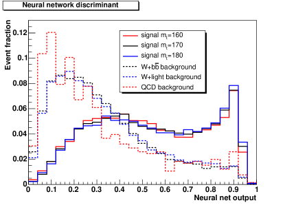
Compared to calculating the background contribution into the observed event probability using matrix element techniques, this method results in a significantly simpler background treatment at the cost of some degradation of the M${}_{\mbox{\scriptsize\,t}}$ estimator statistical uncertainty. The overall sample likelihood is adjusted to remove the expected background contribution according to

$$\begin{array}[]{ll}\ln L_{\mbox{\scriptsize\,adj}}(M_{t},\Delta_{JES})=\sum_{j}&{\!\!\!\!\!}\left[\ln L({\bf y}_{j}|M_{t},\Delta_{JES})\right.\\ &{\!\!\!\!\!}-\left.f_{\mbox{\scriptsize\,b}}(q_{j})\,\overline{\ln L_{\mbox{\scriptsize\,b}}(M_{t},\Delta_{JES})}\,\right].\end{array}$$

Here, $L_{\mbox{\scriptsize\,adj}}$ is the adjusted total likelihood for a given set of events, $L({\bf y}_{j}|M_{t},\Delta_{JES})$ is the signal likelihood calculated for each event $j$, and $f_{\mbox{\scriptsize\,b}}(q_{j})$ is the background fraction for a given event estimated from the neural network output: $f_{\mbox{\scriptsize\,b}}(q_{j})=B(q_{j})/(S(q_{j})+B(q_{j}))$. In this ratio, the $B(q)$ and $S(q)$ distributions are normalized to the overall expected background and signal fractions, respectively. A simulated signal sample with ${\it M}_{\mbox{\scriptsize\,t}}=170$ GeV/$c^{2}$ is used to define $S(q)$, as shown in Figure 22. $\overline{\ln L_{\mbox{\scriptsize\,b}}(M_{t},\Delta_{JES})}$ is the average background log-likelihood estimated from a large sample of simulated Monte Carlo events.

Figure 23: Measured 2D likelihood on the CDF data events, with the contours corresponding to a 1-, 2-, and 3-$\sigma$ uncertainty in the final M${}_{\mbox{\scriptsize\,t}}$ measurement from the profile method. The marker shows the point of maximum likelihood. For consistency with other results, the sign of $\Delta_{JES}$ plotted is reversed w.r.t. (8), (9) [149].

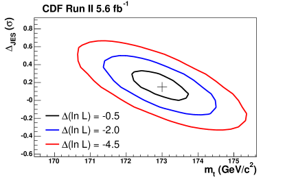
A calibration (mapping function) is applied to $L_{\mbox{\scriptsize\,adj}}$ in order to remove the remaining bias and to ensure proper frequentist coverage of the interval estimate. The calibrated adjusted likelihood is shown in Figure 23. The $\Delta_{JES}$ nuisance parameter is eliminated by profiling.

The systematic uncertainty of the CDF measurement takes into account a number of sources, according to the discussion presented in Section 6. The breakdown of the assigned systematic uncertainty in a set of independent components combined in quadrature is reproduced in Table 3.

Table 3: Systematic uncertainties of the CDF $\ell$+jets M${}_{\mbox{\scriptsize\,t}}$ measurement with 5.6 fb${}^{\mbox{\scriptsize-1}}$ of data [149].

Systematic Source	Uncertainty (GeV/$c^{2}$)
Calibration	0.10
Monte Carlo Generator	0.37
ISR and FSR	0.15
Residual JES	0.49
$b$-JES	0.26
Lepton $p_{T}$	0.14
Multiple Hadron Interactions	0.10
PDFs	0.14
Background Modeling	0.33
Color Reconnection	0.37
Total	0.88

The overall result is ${\it M}_{\mbox{\scriptsize\,t}}=173.0\pm 0.7\,(\mbox{stat.})\pm 0.6\,(\mbox{JES})\pm 0.9\,(\mbox{syst.})$ GeV/$c^{2}$, with a total uncertainty of 1.2 GeV/$c^{2}$.

The current most precise DØ measurement of the top quark mass employs the matrix element method to analyze 3.6 fb${}^{\mbox{\scriptsize-1}}$ of Run II data in the $\ell$+jets channel [99]. The presence of one well-reconstructed charged lepton is required by the event sample selection criteria, together with exactly four high energy jets and substantial missing transverse momentum. A neural network is utilized for heavy flavor tagging [60]. At least one $b$-tagged jet is required resulting in about 70% signal content in the final sample.

A parametric model is employed for the jet energy transfer functions, while jet angles are assumed to be well-measured. The parameterizations are derived for a number of pseudorapidity regions separately for light jets, $b$ jets, and $b$ jets with a soft muon tag (in the latter case, a fraction of the energy of the jets is carried away by a neutrino which escapes detection). The jet energy scale is included in the transfer functions as an overall multiplicative factor, $JES$, which is not related to the prior systematic uncertainty:

$$W_{f}(E_{\mbox{\scriptsize\,jet}}|E_{\mbox{\scriptsize\,parton}},JES)=\frac{1}{JES}\,\varrho_{f}\!\left(\left.\frac{E_{\mbox{\scriptsize\,jet}}}{JES}\right|E_{\mbox{\scriptsize\,parton}}\right).$$

In this analysis, the reference transfer functions $\varrho_{f}(E_{\mbox{\scriptsize\,jet}}|E_{\mbox{\scriptsize\,parton}})$ are represented by the double Gaussian formula:

$$\begin{array}[]{l}\varrho_{f}(E_{\mbox{\scriptsize\,jet}}|E_{\mbox{\scriptsize\,parton}})=\frac{1}{\sqrt{2\pi}(p_{2}+p_{3}p_{5})}\\ \times\left[\exp\left(-\frac{(E_{\mbox{\scriptsize\,jet}}-E_{\mbox{\scriptsize\,parton}}-p_{1})^{2}}{2\,p_{2}^{2}}\right)\right.\\ \left.+\,p_{3}\exp\left(-\frac{(E_{\mbox{\scriptsize\,jet}}-E_{\mbox{\scriptsize\,parton}}-p_{4})^{2}}{2\,p_{5}^{2}}\right)\right].\end{array}$$ (10)

These transfer functions are normalized by

$$\int_{-\infty}^{\infty}\varrho_{f}(E_{\mbox{\scriptsize\,jet}}|E_{\mbox{\scriptsize\,parton}})\,dE_{\mbox{\scriptsize\,jet}}=1$$

for all possible values of $E_{\mbox{\scriptsize\,parton}}$ and of parameters $p_{k}$, $k=1,...,5$. The parameters $p_{k}$ are linear functions of the parton energy: $p_{k}=a_{k}+E_{\mbox{\scriptsize\,parton}}\cdot b_{k}$. The coefficients $a_{k}$ and $b_{k}$ are determined by fitting the jet response in fully simulated Monte Carlo events. It remains unclear how faithfully this model represents the energy response of low $p_{T}$ jets: as emphasized in [146], transfer functions normalized in this manner are unavoidably affected by the jet reconstruction inefficiencies which alter the reference jet energy distributions. Transfer functions are also constructed for the electron energy and muon $p_{T}^{-1}$. The latter quantity is proportional to the muon track curvature in the detector magnetic field (curvature resolution determines the $p_{T}$ uncertainty of the reconstructed muon).

A number of assumptions are introduced to reduce the dimensionality of the signal phase space integral to ten. The following variables are chosen for integration: the transverse momenta of the colliding partons (for which priors are derived from PYTHIA), the energy associated with one of the quarks from the hadronic $W$ boson decay, the masses of the two $W$ bosons and the two top quarks, and either the energy of the electron or $1/p_{T}$ of the muon. The signal matrix element models the dominant $q\bar{q}\rightarrow t\bar{t}$ production process [174], while $t\bar{t}$ spin correlations are ignored.

The background contribution into the event probability is calculated using the $W$ + 4 jets matrix element provided by VECBOS [175]. It is assumed that this contribution alone is sufficient to model the shape of the background likelihood, while other backgrounds (mainly QCD multijet events) are not treated explicitly. The background normalization is adjusted so that the correct $t\bar{t}$ signal fraction can be reproduced in the analysis of simulated event samples. The overall event sample likelihood is profiled over the signal fraction nuisance parameter. $JES$ is marginalized with a Gaussian prior consistent with the $JES$ uncertainty from jet energy calibrations.

Systematics uncertainties of the DØ M${}_{\mbox{\scriptsize\,t}}$ measurement with Run IIb data are shown in Table 4. The source breakdown is substantially different from that utilized by CDF. The generator systematic uncertainty, here called Higher Order Effects, was calculated comparing ALPGENv2+HERWIG with MC@NLO.

Table 4: Systematic uncertainties of the DØ $\ell$+jets M${}_{\mbox{\scriptsize\,t}}$ measurement with 2.6 fb${}^{\mbox{\scriptsize-1}}$ of Run IIb data [99].

Systematic Source	Uncertainty (GeV/$c^{2}$)
Higher Order Effects	0.25
ISR and FSR	0.26
Hadronization and UE	0.58
Color Reconnection	0.28
Multiple $p\bar{p}$ Interactions	0.07
Background Modeling	0.16
$W$+jets Heavy Flavor	0.07
Scale Factor
$b$-jet Modeling	0.09
PDF	0.24
Residual JES	0.21
Data-MC Jet Response	0.28
Difference
$b$-tagging Efficiency	0.08
Trigger Efficiency	0.01
Lepton Momentum Scale	0.17
Jet Energy Resolution	0.32
Jet Identification Efficiency	0.26
QCD Background	0.14
Signal Fraction	0.10
MC Calibration	0.20
Total	1.02

The overall result (Run IIa and Run IIb combined) is ${\it M}_{\mbox{\scriptsize\,t}}=174.94\pm 0.83\,(\mbox{stat.})\pm 0.78\,(\mbox{JES})\pm 0.96\,(\mbox{syst.})$ GeV/$c^{2}$, with a total uncertainty of 1.49 GeV/$c^{2}$. The sample likelihood as a function of M${}_{\mbox{\scriptsize\,t}}$ and $JES$ (labelled by m${}_{\mbox{\scriptsize\,t}}$ and k${}_{\mbox{\scriptsize\,JES}}$, respectively, on the axes) is shown in Figure 24.

Figure 24: Calibrated DØ result obtained with the Run IIb data in the $\ell$+jets channel. The JES prior factor is included into the likelihood. The boxes, representing the bins in the two-dimensional histograms of the likelihoods, have areas proportional to the bin contents [99].

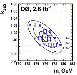
A set of representative Tevatron M${}_{\mbox{\scriptsize\,t}}$ measurements in the $\ell$+jets channel is collected in Table 5 which illustrates the evolution of analysis techniques and attained precision with integrated luminosity.

Table 5: Representative Tevatron M${}_{\mbox{\scriptsize\,t}}$ measurements in the $\ell$+jets channel. If a reference is marked by (*) then the $JES$ calibration uncertainty is included as a part of statistical rather than systematic uncertainty.

Experiment	Method	$\int\mathcal{L}dt$	M${}_{\mbox{\scriptsize\,t}}$	$\sigma_{\mbox{\scriptsize\,stat}}$	$\sigma_{\mbox{\scriptsize\,syst}}$	Ref.
		(fb${}^{\mbox{\scriptsize-1}}$)	(GeV/$c^{2}$)	(GeV/$c^{2}$)	(GeV/$c^{2}$)
CDF (Run I)	template	0.02	174	10	$\mbox{}^{+13}_{-12}$	[7]
DØ (Run I)	template	0.05	199	$\mbox{}^{+19}_{-21}$	22	[6]
CDF (Run I)	template	0.07	176	8	10	[5]
CDF (Run I)	template	0.11	176.1	5.1	5.3	[100, 103]
DØ (Run I)	template	0.13	173.3	5.6	5.5	[101, 104]
DØ (Run I)	MEM	0.13	180.1	3.6	3.9	[96]
CDF	template	0.16	179.6	$\mbox{}^{+6.4}_{-6.3}$	6.8	[119]
CDF	DLM	0.16	177.8	$\mbox{}^{+4.5}_{-5.0}$	6.2	[176]
DØ	template	0.16	170.0	6.5	$\mbox{}^{+10.5}_{-6.1}$	[136]
DØ	ideogram	0.16	177.5	5.8	7.1	[136]
DØ	template	0.23	170.6	4.2	6.0	[177]
CDF	DLM	0.32	173.2	$\mbox{}^{+2.6}_{-2.4}$	3.2	[116, 157]
CDF	template	0.32	173.5	$\mbox{}^{+3.7}_{-3.6}$	1.3	[116, 114]*
DØ	template	0.32	169.5	4.4	$\mbox{}^{+1.7}_{-1.6}$	[178]*
DØ	MEM	0.37	170.3	$\mbox{}^{+4.1}_{-4.5}$	$\mbox{}^{+1.2}_{-1.8}$	[97]*
DØ	ideogram	0.43	173.7	4.4	$\mbox{}^{+2.1}_{-2.0}$	[59]*
CDF	MEM	1.0	170.8	2.2	1.4	[179]*
CDF	template	1.0	168.9	2.2	4.2	[140]
DØ	MEM	1.0	171.5	1.8	1.1	[98]*
CDF	DLM	1.7	171.6	2.0	1.3	[158]*
CDF	MEM	1.9	172.7	1.2	1.8	[148]
CDF	template	1.9	171.8	1.9	1.1	[93]*
DØ	MEM	2.2	172.2	1.0	1.4	[180]
CDF	template	3.2	172.2	1.1	1.5	[94]
CDF	MEM	3.2	172.4	1.4	1.3	[150]*
DØ	MEM	3.6	174.9	0.8	1.2	[99]
CDF	MEM	5.6	173.0	0.7	1.1	[149]
CDF	template	5.6	172.2	1.2	0.9	[65]*

[hbtp] Recent CDF and DØ results are in good agreement with each other.

7.2 All-hadronic topology

The all-hadronic branching fraction of about 46% is the largest among all $t\bar{t}$ decay channels. Due to the absence of neutrinos, this final state is kinematically constrained, and in principle, the $t\bar{t}$ event can be reconstructed. The challenges are reduction of the very large QCD background due to multijet production and reduction of the 90 possible permutations that can be made in assigning 2 jets to b quarks and pairing the remaining 4 jets.

Dedicated trigger requirements are needed in order to enhance the top quark signal contribution over the overwhelming background. Even after surviving such trigger requirements, the background is about three orders of magnitude larger than the signal. In order to reconstruct the $t\bar{t}$ events, at least six high-$p_{T}$ jets must be present in the detector, while charged and neutral leptons are vetoed. Identifying jets originated from $b$ quarks helps both in suppressing the QCD background and in reducing the number of possible permutations in reconstructing the final state kinematics according to the $t\bar{t}\to W^{+}bW^{-}\bar{b}\to q_{1}\bar{q}_{2}bq_{3}\bar{q}_{4}\bar{b}$ hypothesis. The distinct kinematic properties of $t\bar{t}$ events are further exploited to bring the S/B ratio to an acceptable level.

Due to the unique challenges, the observation of this decay mode was achieved only after $t\bar{t}$ events were seen in the $\ell$+jets and dilepton channels, by analyzing the full Tevatron Run I dataset of 110 pb^-1. CDF utilized a combination of $b$-tagging and kinematic/topological cuts to select a relatively clean sample of top quark pair events subsequently used to estimate M${}_{\mbox{\scriptsize\,t}}$ [181]. DØ used neural networks to exploit the S/B discriminating power of several kinematic and topological observables [106].

Table 6: Tevatron M${}_{\mbox{\scriptsize\,t}}$ measurements in the all-hadronic channel.

Experiment	Method	$\int\mathcal{L}dt$	M${}_{\mbox{\scriptsize\,t}}$	$\sigma_{\mbox{\scriptsize\,stat}}$	$\sigma_{\mbox{\scriptsize\,syst}}$	Ref.
		(fb${}^{\mbox{\scriptsize-1}}$)	(GeV/$c^{2}$)	(GeV/$c^{2}$)	(GeV/$c^{2}$)
CDF (Run I)	template	0.11	186	10	12	[181]
DØ  (Run I)	template	0.11	178.5	13.7	7.7	[106]
CDF	ideogram	0.31	177.1	4.9	4.7	[134]
CDF	template	1.0	174.0	2.2	1.8	[105]
CDF	MEM-assisted	1.0	171.1	2.8	3.2	[117]
CDF	template	2.9	174.8	1.7	2.0	[87]
CDF	template	5.8	172.5	1.4	1.4	[113]

[hbtp] The $t\bar{t}$ events in the all-hadronic final state were observed again during the Run II by both CDF [182, 105, 87] and DØ [88] collaborations. The new measurements of M${}_{\mbox{\scriptsize\,t}}$ and $t\bar{t}$ production cross section benefited from the larger center-of-mass energy resulting in $\sim 30\%$ higher cross section, from improved detectors, and from better analysis techniques. For both data taking periods, the QCD multijet background is estimated from data; the much larger event sample collected in Run II allows for a very accurate control of the background modeling.

The Tevatron publications of M${}_{\mbox{\scriptsize\,t}}$  measurements in the all-hadronic channel are listed in Table 6. So far, only the CDF collaboration measured the top quark mass with the Run II data.

The CDF multijet trigger requires four energetic jets in the event and large energy deposit in the calorimeter in order to select all-hadronic $t\bar{t}$ decays while suppressing the much more common QCD multijet production. The use of a neural network to obtain a cleaner sample of top quark hadronic decays resulted in a large improvement in the statistical sensitivity of the measurement [105]. Similar to the $\ell$+jets channel, hadronic decays of the $W$ bosons are used to measure the jet energy scale in situ with the available dataset. This technique provides an important reduction in the systematic uncertainty that would otherwise limit the precision of the M${}_{\mbox{\scriptsize\,t}}$ estimate in this channel to $\sim 3\%$.

The latest and most precise M${}_{\mbox{\scriptsize\,t}}$  measurement in this channel [87, 113] uses several kinematic and topological properties of the events as inputs to a neural network to separate the signal from the background. It also exploits the fact that all-hadronic top quark events produce at first approximation only quark jets, while the QCD background produces on average several gluon jets in the final state. Signal-like quark jets can be statistically discriminated from background-like gluon jets using calorimeters with sufficient granularity. In fact, observed differences in quark and gluon jet widths have been previously reported by experiments at the KEK $e^{+}e^{-}$ collider (TRISTAN) [183] and the CERN $e^{+}e^{-}$ collider (LEP) [184, 185]. A cut is placed on the neural network output shown in Figure 25, and on the quality of the fit that assigns the jets to the final state partons when the top quark pair decay chain is reconstructed. Both cuts were chosen to minimize the statistical uncertainty on the top quark mass measurement. The event sample is split into two subsamples: with one $b$-tagged jet and with two or more $b$-tagged jets. For the latter subsample, S/B$\,\approx 1$.

Figure 25: Output of the neural network used to discriminate $t\bar{t}\to q_{1}\bar{q}_{2}bq_{3}\bar{q}_{4}\bar{b}$ events from QCD multijet production [87].

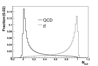
Multiple collisions occurring in the same bunch crossing often produce extra jets, and thus extra energy in the calorimeter. For this reason, as the collider instantaneous luminosity increased over time, so did the trigger rate. The data collected until the end of year 2007 has been obtained with the Tevatron colliding particles with an average instantaneous luminosity at the beginning of the store of about $10^{32}$ cm^-2 s^-1. Under these conditions, the trigger rate was relatively low and the event selection efficiency is about 4%, higher than in the $\ell$+jets case but with much higher backgrounds. Starting from 2008, the instantaneous luminosity at the beginning of the store was on average three times larger, thus the trigger rates and as a consequence the multijet background increased by a factor of 3. This was dealt with at the event selection level, by tightening the neural network output cut and the cut on the kinematic fitter goodness-of-fit. This tighter set of cuts provides better reconstructed events at the cost of a lower event selection efficiency. The reconstructed top quark mass and the reconstructed $W$ boson mass distributions can be seen in Figure 26.

Figure 26: Distribution of the reconstructed top quark mass (left) and $W$ mass (right) for events surviving the event selection. The plots show the events with at least one $b$-tagged jet passing the neural network event selection and the goodness-of-fit requirement. These two criteria are optimized to reduce the statistical uncertainty on the M${}_{\mbox{\scriptsize\,t}}$  and $JES$ measurements, respectively [113].

Figure 27: Simultaneous measurement of the top quark mass and the jet energy scale in the all-hadronic channel. The $\Delta_{JES}$ parameter is related to the jet energy scale according to (8) [113].

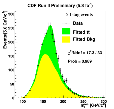
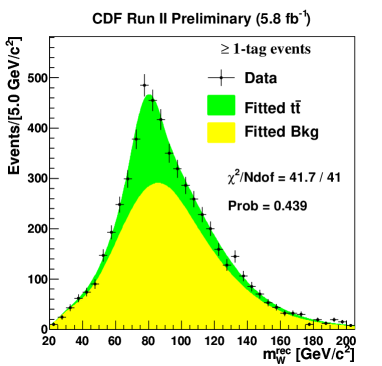
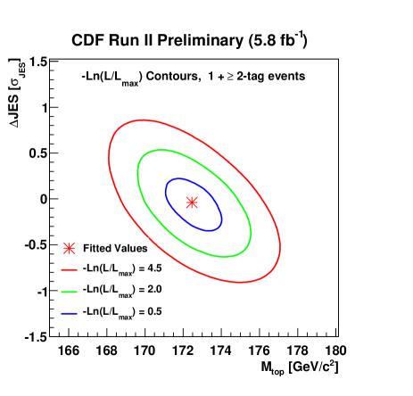
Owing to the improved analysis techniques, the statistical precision of the M${}_{\mbox{\scriptsize\,t}}$ measurement scaled better than with $1/\sqrt{\int\mathcal{L}dt}$, while the dominant systematic uncertainty due to the jet energy scale has been linked to $1/\sqrt{\int\mathcal{L}dt}$. The most precise determination of the top quark mass in the all-hadronic channel as of this writing gives ${\it M}_{\mbox{\scriptsize\,t}}=172.5\pm 1.4\,(\mbox{stat.})\pm 1.0\,(\mbox{JES})\pm 1.2\,(\mbox{syst.})$ GeV/$c^{2}$, or ${\it M}_{\mbox{\scriptsize\,t}}=172.5\pm 2.0\,(\mbox{total})$ GeV/$c^{2}$. The ultimate precision that can be reached in this channel is now limited by 1.1 GeV/$c^{2}$ due to the systematic uncertainties other than the overall jet energy scale. It can be appreciated from Figure 27 that the measured value of $\Delta_{JES}$ is consistent with the prior expectation (mean value close to zero) with the precision a factor of three better than the prior constraint.

7.3 Events with taus

About 35% of decays of the tau lepton are pure leptonic, with an electron or a muon and two neutrinos in the final state. Charged leptons produced in such decays often pass standard electron or muon selection requirements. Therefore, the $t\bar{t}$ event selection criteria in the $\ell$+jets and dilepton channels actually accept a fraction of events which contain leptonically decaying taus. On the other hand, explicit identification of tau leptons which decay hadronically is difficult: these decays resemble common hadronic jets originating from quarks and gluons. For this reason, hadronic tau identification algorithms typically have to operate at low efficiency. For signals with many jets in the final state, as the $t\bar{t}$ decays under consideration here, the explicit tau identification is often not sufficient to suppress the QCD background in the sample. One can instead rely upon the experimental signature characterized by multiple jets and large ${\not}{E_{T}}$ in the final state as an efficient way to collect the $t\bar{t}$ events with tau leptons.

The first measurement of the $t\bar{t}$ cross section which utilized events with large ${\not}{E_{T}}$ and multiple jets, with at least one $b$-tagged jet, was performed by the CDF collaboration using 310 pb^-1 of Tevatron Run II data [186]. A more recent CDF study of this experimental signature utilized 2.2 fb^-1 of Run II data [89]. In both measurements, a veto on the presence of reconstructed electrons or muons was applied in order to avoid overlap with other channels. The more recent study utilized a neural network for background rejection achieving a S/B ratio of about 4. About 90% of the signal sample was composed of $t\bar{t}\to W^{+}bW^{-}\bar{b}\to\ell\nu+$4 jets events, with $\ell=\tau$ in 40% of the cases.

In this sample, one of the two top quarks is expected to decay into $\ell\nu b$, with charged lepton not identified. This decay provides little information about the top quark mass. Still, the other top quark in the event produces three jets which can be used to reconstruct its decay chain and to measure the jet energy scale in situ. This feature is exploited in the recent CDF M${}_{\mbox{\scriptsize\,t}}$ measurement [118]. The kinematic analysis starts by identifying decay products of the hadronically decaying $W$. All pairwise combinations of jets without $b$ tags are considered, and the pair which gives the invariant mass closest to the world average $W$ mass is chosen. Then the jet with the highest $E_{T}$ is chosen among the remaining jets and added to the pair in order to construct a 3-jet system whose invariant mass is correlated with the top quark mass. Another such system is built by adding the jet with the second highest $E_{T}$ to the pair. 3-dimensional templates are constructed using the di-jet and the two tri-jet invariant masses.

Table 7: Tevatron M${}_{\mbox{\scriptsize\,t}}$ measurements in the ${\not}{E_{T}}$+jets channel (all by CDF).

$\int\mathcal{L}dt$	M${}_{\mbox{\scriptsize\,t}}$	$\sigma_{\mbox{\scriptsize\,stat}}$	$\sigma_{\mbox{\scriptsize\,syst}}$	Ref.
(fb${}^{\mbox{\scriptsize-1}}$)	(GeV/$c^{2}$)	(GeV/$c^{2}$)	(GeV/$c^{2}$)
0.3	172.3	10.2	10.8	[187]
5.7	172.3	1.8	1.8	[118]

Figure 28: Distribution of the reconstructed top quark mass for events with at least one $b$-tagged jet. The events are required to satisfy the neural network event selection and the goodness-of-fit criterion [118].

Figure 29: Simultaneous measurement of the top quark mass and of the jet energy scale in the ${\not}{E_{T}}$+jets channel. The $\Delta_{JES}$ parameter is related to the jet energy scale according to (8) [118].

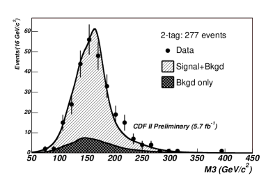
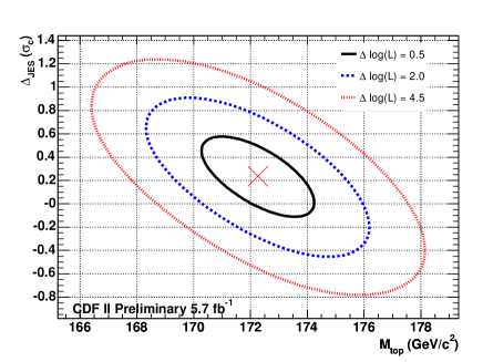
Owing to the large signal acceptance, the good S/B ratio, and the capability to constrain in situ the jet energy scale uncertainty, this measurement achieves a precision superior to that attainable in the dilepton channel. The result is ${\it M}_{\mbox{\scriptsize\,t}}=172.3\pm 1.8\,(\mbox{stat.})\pm 1.5\,(\mbox{JES})\pm 1.0\,(\mbox{syst.})$ GeV/$c^{2}=172.3\pm 2.6\,(\mbox{total})$ GeV/$c^{2}$, in agreement with the M${}_{\mbox{\scriptsize\,t}}$ estimates in other decay modes. This result is shown in Figure 29, together with the jet energy scale estimate.

It should be noted that for this channel, just as for the $\ell$+jets and all-hadronic signatures, the uncertainty on the JES shift is much lower than the typical 3% uncertainty of the prior calibration. In other words, the collective light quark JES measurements obtained with about 5,000 $t\bar{t}$ events in the $\ell$+jets, all-hadronic and ${\not}{E_{T}}$+jets final states, validated the data-to-MC correspondence of the overall JES at better than one percent level. The Tevatron experiments did not use this value in data analyses other than the M${}_{\mbox{\scriptsize\,t}}$ measurements where they were derived, conservatively assuming that different jet multiplicities could alter the jet shapes and result in a systematic uncertainty different from the one quoted here. Still, the M${}_{\mbox{\scriptsize\,t}}$ measurements in these three channels utilize events that range in jet multiplicity from four to eight, with compatible results. Even though the details of the $p_{T}$ and $\eta$ dependence of the light quark jet response remain to be understood at this level of precision, the Tevatron results suggest that, with the larger dataset available at the LHC, it should be possible to calibrate light quark jets using the hadronically decaying $W$s from $t\bar{t}$ events with uncertainty of 1% or better.

7.4 Dilepton measurements

Due to the presence of two charged leptons and two neutrinos in the final state, the event samples used to measure M${}_{\mbox{\scriptsize\,t}}$ in the dilepton channel have excellent signal purity. Compared to other $t\bar{t}$ final states, physics effects beyond the SM affecting the M${}_{\mbox{\scriptsize\,t}}$ estimate are easier to detect. However, a relatively low branching fraction ($\approx 5$%, not counting events with the $\tau$ lepton) and the absence of the hadronic $W$ decay which provides a natural reference point for jet energy calibration in other channels limit achievable statistical and systematic precision of the M${}_{\mbox{\scriptsize\,t}}$ estimate. The dilepton measurements thus complement more precise results obtained in other channels.

At the time of this writing, the dilepton M${}_{\mbox{\scriptsize\,t}}$ measurement with the smallest uncertainty is performed with 5.4 fb${}^{\mbox{\scriptsize-1}}$ of data collected by the DØ detector in Tevatron Run II [188]. The events are naturally split into subsamples with $ee$, $e\mu$, or $\mu\mu$ in the final state, with different expected backgrounds. For the $ee$ and $\mu\mu$ final states, the events are selected by a set of single-lepton triggers. For the $e\mu$ channel, a mix of single and multilepton triggers and lepton+jet triggers is utilized. The events are required to have two oppositely charged isolated leptons with $p_{T}>15$ GeV/$c$, and either $|\eta|<1.1$ or $1.5<|\eta|<2.5$ for electrons and $|\eta|<2$ for muons, ensuring high efficiency and low fake rate for lepton identification. At least two jets are required with $p_{T}>20$ GeV/$c$ and $|\eta|<2.5$. Background is further suppressed by the $H_{T}>115$ GeV requirement in the $e\mu$ final state and by requiring substantial missing transverse momentum in the $ee$ and $\mu\mu$ states. 479 candidate events are selected with 73, 266, and 140 events, respectively, in the $ee$, $e\mu$, and $\mu\mu$ channels, of which about $13\pm 5$, $48\pm 15$, and $56\pm 15$ events, respectively, are expected to arise from background. The sample purity (S/B $\approx$ 3) is already sufficient so that explicit $b$ flavor identification is not required for jets.

The M${}_{\mbox{\scriptsize\,t}}$ estimate is constructed by the matrix element method. In the calculation of event observation probability, two contributions are taken into account: the $q\bar{q}\rightarrow t\bar{t}$ signal process and $p\bar{p}\rightarrow Z$ + 2 jets production which is expected to be the dominant source of background. The jet energy transfer functions are modeled according to (10). Directions of all jets and charged leptons, as well as electron energies, are assumed to be perfectly measured. The uncertainty of the muon track curvature determination is modeled by a Gaussian resolution function. Transfer functions are also constructed for the fraction of parent energy carried by electrons and muons produced in the $\tau\rightarrow\ell\nu_{\ell}\nu_{\tau}$ decays (relevant for the $Z\rightarrow\tau^{+}\tau^{-}$ decay mode). Under the assumption that the direction of the charged lepton coincides with the direction of the parent tau and that the daughter leptons are massless, the appropriate laboratory spectrum is described in [189].

The phase space integration for the signal hypothesis is performed over the following variables: transverse momentum of the $t\bar{t}$ system with a prior derived from the ALPGEN event generator [75], energies of the $b$ quarks, the lepton-neutrino invariant masses, the differences between neutrino transverse momenta, and the muon track curvature ($p_{T}^{-1}$).

The background matrix element is calculated using VECBOS [175]. The background phase space is sampled over the energies of the two partons that produce the jets and, in the case of $Z\rightarrow\tau^{+}\tau^{-}$ decays, over the energy fractions of the charged leptons produced in tau decays. The $p_{T}$ probability of the $Z$ + 2 jets system is used as the additional weight, together with the leading order matrix element, parton distribution functions, and appropriate phase space factors. Background normalization is adjusted in a manner similar to that employed in the DØ M${}_{\mbox{\scriptsize\,t}}$ measurement in the $\ell+$jets channel (Section 7.1). The likelihood as a function of M${}_{\mbox{\scriptsize\,t}}$ is obtained by profiling over the $t\bar{t}$ signal fraction. The bias and pulls of the final estimate are corrected by a mapping function, and the Bayesian credible interval is extracted. The calibrated likelihood is shown in Figure 30.

Figure 30: Calibrated and normalized likelihood for data as a function of M${}_{\mbox{\scriptsize\,t}}$ with best estimate as well as 68% confidence level region marked by the shaded area [188].

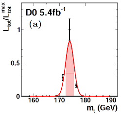
In this measurement, the largest component (2.2 GeV/$c^{2}$) of the systematic uncertainty is contributed by the calibration of the jet response. The overall result is ${\it M}_{\mbox{\scriptsize\,t}}=174.0\pm 1.8\,(\mbox{stat.})\pm 2.4\,(\mbox{syst.})$ GeV/$c^{2}$, or ${\it M}_{\mbox{\scriptsize\,t}}=174.0\pm 3.1\,(\mbox{total})$ GeV/$c^{2}$.

The current most precise CDF M${}_{\mbox{\scriptsize\,t}}$ measurement in the dilepton channel is performed by simultaneous application of the template method in the $\ell$+jets and dilepton final states which allows for in situ calibration of the jet energy scale in both channels [65]. 5.6 fb${}^{\mbox{\scriptsize-1}}$ of data collected by the CDF detector in Tevatron Run II is used, with $\ell$+jets selection criteria similar to those described in Section 7.1. The dilepton events are required to have two well-identified oppositely charged leptons and at least two jets with $E_{T}>15$ GeV and $|\eta|<2.5$. To further reject backgrounds, both missing transverse energy and $H_{T}$ requirements are imposed: ${\not}{E_{T}}>25$ GeV and $H_{T}>200$ GeV.

Two-dimensional templates are constructed for the M${}_{\mbox{\scriptsize\,t}}$ determination by kernel density estimation (KDE). The variables used are the event-by-event $m_{t}$ values obtained with the neutrino weighting algorithm ($\nu$WT, described in Section 5.3) and the transverse mass $m$${}_{\mbox{\scriptsize\,T2}}$. Distributions of these quantities in the data and in a simulated sample with ${\it M}_{\mbox{\scriptsize\,t}}=170$ GeV/$c^{2}$ are shown in Figure 31.

Figure 31: Distributions of $m_{t}$ values obtained with the $\nu$WT method (left) and of the transverse mass $m_{\mbox{\scriptsize\,T2}}$ (right) using CDF $b$-tagged events. The data is overlaid with KDE templates [65].

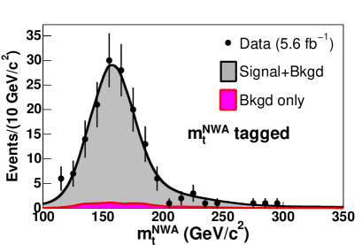
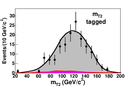
In the $\ell$+jets channel, $m_{t}$ values are obtained by kinematic fitting based on $\chi^{2}$ minimization (Section 5.3). Twelve jet-to-parton assignments are considered which result in distinct $\chi^{2}$. The $m_{t}$ values from the two fits with the lowest $\chi^{2}$ are combined with $m_{jj}$ (for jets assumed to come from the hadronic $W$ decay) from the lowest $\chi^{2}$ permutation, and three-dimensional templates are built by KDE. As both signal and background template shapes depend on the presence of $b$-tagged jets in the sample, the templates are made separately for a number of subsamples: 1-tag and 2-tag for $\ell$+jets events (at least one secondary vertex $b$ tag is required), non-tagged and tagged for dilepton events. The overall likelihood is obtained as a function of M${}_{\mbox{\scriptsize\,t}}$ and $\Delta_{JES}$ by multiplying together the likelihoods from all subsamples. The $\Delta_{JES}$ nuisance parameter is then eliminated by profiling. Finally, remaining biases and pulls are corrected by a mapping function.

Despite cross-calibration from the $\ell$+jets channel, the systematic uncertainty of this measurement is still dominated by jet response modeling (of $b$ jets in particular) which contributes 3.0 GeV/$c^{2}$. The obtained result is ${\it M}_{\mbox{\scriptsize\,t}}=170.3\pm 2.0\,(\mbox{stat.})\pm 3.1\,(\mbox{syst.})$ GeV/$c^{2}$, with a total uncertainty of 3.7 GeV/$c^{2}$. Tevatron M${}_{\mbox{\scriptsize\,t}}$ measurements in the dilepton channel are summarized in Table 8.

Table 8: Representative Tevatron M${}_{\mbox{\scriptsize\,t}}$ measurements in the dilepton channel. The “+” sign between the methods indicates that the overall result is obtained by combining multiple techniques. “$\otimes$” joins variables used in multivariate templates.

Experiment	Method	$\int\mathcal{L}dt$	M${}_{\mbox{\scriptsize\,t}}$	$\sigma_{\mbox{\scriptsize\,stat}}$	$\sigma_{\mbox{\scriptsize\,syst}}$	Ref.
		(fb${}^{\mbox{\scriptsize-1}}$)	(GeV/$c^{2}$)	(GeV/$c^{2}$)	(GeV/$c^{2}$)
CDF (Run I)	$\nu$WT	0.11	167.4	10.3	4.8	[102]
DØ (Run I)	${\mathcal{M}}$WT + $\nu$WT	0.13	168.4	12.3	3.6	[127, 128]
DØ	${\mathcal{M}}$WT	0.23	155	$\mbox{}^{+14}_{-13}$	7	[190]
CDF	MEM	0.34	165.2	6.1	3.4	[191, 151]
CDF	DLM	0.34	166.6	$\mbox{}^{+7.3}_{-6.7}$	3.2	[159]
CDF	$\nu$WT + KIN + PHI	0.36	170.1	6.0	4.1	[107]
DØ	${\mathcal{M}}$WT + $\nu$WT	0.37	178.1	6.7	4.8	[110]
DØ	${\mathcal{M}}$WT + $\nu$WT	1.0	174.7	4.4	2.0	[112]
CDF	MEM	1.0	164.5	3.9	3.9	[152]
CDF	KIN + cross section	1.2	170.7	$\mbox{}^{+4.2}_{-3.9}$	3.5	[111]
CDF	$\nu$WT	1.9	172.0	$\mbox{}^{+3.6}_{-3.4}$	3.8	[93]
CDF	MEM	2.0	171.2	2.7	2.9	[160]
DØ	MEM	2.8	172.9	3.6	2.3	[192]
CDF	PHI	2.9	165.5	$\mbox{}^{+3.4}_{-3.3}$	3.1	[108]
CDF	$\nu$WT $\otimes$ $m_{\mbox{\scriptsize\,T2}}$	3.4	169.3	2.7	3.2	[115]
DØ	MEM	3.6	174.8	3.3	2.6	[193]
DØ	$\nu$WT	5.3	173.3	2.4	2.1	[142]
DØ	MEM	5.4	174.0	1.8	2.4	[188]
CDF	$\nu$WT $\otimes$ $m_{\mbox{\scriptsize\,T2}}$	5.6	170.3	2.0	3.1	[65]

7.5 Measurements which do not use jets

A number of unconventional top quark mass measurement ideas were proposed in the recent literature and tested on the Run II Tevatron data. These proposals aim to reduce the systematic uncertainty (especially its part related to the jet energy response calibration), often at the cost of a substantial degradation in the statistical precision. Even though at this time such methods are not competitive with the “traditional” techniques described earlier in this section, their special features could make them attractive for the analysis of massive $t\bar{t}$ event samples which will be accumulated by the LHC experiments. A few of these ideas are described below.

M${}_{\mbox{\scriptsize\,t}}$ measurements based on the tracking information alone were explored by CDF in [122]. Two variables were chosen to build the templates in the $\ell$+jets channel: L${}_{\mbox{\scriptsize\,xy}}$ which is the transverse distance between the primary and secondary vertices projected onto the jet direction and $p_{T}$ of the lepton produced in the $W\rightarrow\ell\nu_{\ell}$ decay. Standalone lepton $p_{T}$ templates were later used by CDF to estimate M${}_{\mbox{\scriptsize\,t}}$ in the $\ell$+jets [125] and dilepton [124] channels.

Both L${}_{\mbox{\scriptsize\,xy}}$ and lepton $p_{T}$ variables are sensitive to M${}_{\mbox{\scriptsize\,t}}$ because $W$ bosons and $b$ quarks produced in the $t\rightarrow Wb$ decays receive higher transverse boosts from heavier top quarks, as illustrated in Figure 17. While the sensitivity of such variables to the calorimeter hadronic jet energy scale calibration is indeed minimal, reliance upon manifestly non-Lorentz invariant quantities has its own disadvantages. Both variables are highly sensitive to the mismodeling of parton distribution functions which affect typical center-of-mass energies and therefore average boosts of parent top quarks. The sensitivity to the uncertainties in background shape and composition is also increased. In addition, the L${}_{\mbox{\scriptsize\,xy}}$ distributions in Monte Carlo are strongly affected by the $b$ jet fragmentation model, while the lepton $p_{T}$ measurements suffer from imprecise energy scale calibration of the electromagnetic calorimeter. On the other hand, the L${}_{\mbox{\scriptsize\,xy}}$-based estimate is essentially complementary to all other methods of top mass determination, and constitutes an independent source of information about M${}_{\mbox{\scriptsize\,t}}$ (the same can not be said about lepton $p_{T}$ which is used either explicitly or implicitly by kinematic fitting and matrix element techniques).

The invariant mass, $M_{\ell\mu}$, of the charged lepton from the $W$ decay and the muon from a semileptonic decay of the $b$ quark (originated from the same parent top as the leptonically decaying $W$) was used as template variable in the CDF study [126]. The efficiency to “tag” a $t\bar{t}$ event passing typical $\ell$+jets event selection criteria by finding a soft muon produced in a decay of a $b$ quark is about 14% [194]. This leads to a sizeable event sample: 248 events were selected in the 2.0 fb${}^{\mbox{\scriptsize-1}}$ of CDF Run II data. The selection included events with 3 jets which resulted in a somewhat higher efficiency but lower than usual S/B of about 2. The average $M_{\ell\mu}$ of the selected sample depends approximately linearly on M${}_{\mbox{\scriptsize\,t}}$, as illustrated in Figure 32.

Figure 32: The correlation between the mean value of the $M_{\ell\mu}$ histograms from simulated $t\bar{t}$ and background samples and the input M${}_{\mbox{\scriptsize\,t}}$. The continuous line shows a linear fit to the points [126].

In this analysis, the dominant components of the systematic uncertainty are due to imprecise knowledge of the background shape and fraction in the $M_{\ell\mu}$ template ($\sigma_{\mbox{\scriptsize\,bg}}=1.9$ GeV/$c^{2}$, statistically limited by the size of the available event sample) and due to uncertainties in signal modeling, especially $b$ jet fragmentation, conservatively estimated by comparing M${}_{\mbox{\scriptsize\,t}}$ estimates obtained for event samples generated by HERWIG [69] and PYTHIA [17] ($\sigma_{\mbox{\scriptsize\,s}}=2.1$ GeV/$c^{2}$).

The M${}_{\mbox{\scriptsize\,t}}$ estimates obtained by methods which rely mainly on tracking information are collected in Table 9.

Table 9: M${}_{\mbox{\scriptsize\,t}}$ estimates which rely on tracking information (all by CDF).

Template	Channel	$\int\mathcal{L}dt$	M${}_{\mbox{\scriptsize\,t}}$	$\sigma_{\mbox{\scriptsize\,stat}}$	$\sigma_{\mbox{\scriptsize\,syst}}$	Ref.
quantity		(fb${}^{\mbox{\scriptsize-1}}$)	(GeV/$c^{2}$)	(GeV/$c^{2}$)	(GeV/$c^{2}$)
L${}_{\mbox{\scriptsize\,xy}}$	$\ell$+jets	0.7	180.7	$\mbox{}_{-13.4}^{+15.5}$	8.6	[121]
Lepton $p_{T}$	dilepton	1.8	156	20	4.6	[123]
L${}_{\mbox{\scriptsize\,xy}}$	$\ell$+jets	1.9	166.9	$\mbox{}_{-8.5}^{+9.5}$	2.9	[122]
Lepton $p_{T}$	$\ell$+jets	1.9	173.5	$\mbox{}_{-8.9}^{+8.8}$	3.8	[122]
$M_{\ell\mu}$	$\ell$+jets	2.0	180.5	12.0	3.6	[126]
Lepton $p_{T}$	$\ell$+jets	2.7	176.9	8.0	2.7	[125]
Lepton $p_{T}$	dilepton	2.8	154.6	13.3	2.3	[124]

Potential relevance of these methods for top mass measurements with LHC event samples will strongly depend on the improvements in the modeling of parton distribution functions and $b$ jet fragmentation, as well as on the availability of precise detector calibrations for lepton $p_{T}$.

7.6 Top-antitop mass difference

The DØ collaboration was the first to search for a violation of the CPT-invariance in the $t\bar{t}$ production and decay processes by measuring the difference between the masses of the $t$ and $\bar{t}$ quarks [195]. The latest DØ measurement [196] of $\Delta\equiv{\it M}_{\mbox{\scriptsize\,t}}-{\it M}_{\,\bar{\mbox{\scriptsize t}}}$ is performed with an event sample which corresponds to about 3.6 fb${}^{\mbox{\scriptsize-1}}$ of Tevatron Run II data. The $\ell$+jets final state is selected in which positively (negatively) charged leptons are used to tag the $t$ ($\bar{t}\,$) quarks in each event. The matrix element technique is utilized to construct the overall likelihood as a function of $M_{\mbox{\scriptsize\,sum}}=({\it M}_{\mbox{\scriptsize\,t}}+{\it M}_{\,\bar{\mbox{\scriptsize t}}})/2$, $\Delta$, $JES$, and the signal fraction, in a manner similar to the DØ M${}_{\mbox{\scriptsize\,t}}$ measurement described in Section 7.1. The signal fraction nuisance parameter is eliminated by profiling, while $JES$ is fixed to a constant value consistent with the $W$ mass constraint. The resulting likelihoods, represented as functions of M${}_{\mbox{\scriptsize\,t}}$ and M${}_{\,\bar{\mbox{\scriptsize t}}}$, are shown in Figure 33 separately for the $e$+jets and $\mu$+jets channels.

Figure 33: Sample likelihoods as a function of M${}_{\mbox{\scriptsize\,t}}$ and M${}_{\,\bar{\mbox{\scriptsize t}}}$ for (a) $e$+jets and (b) $\mu$+jets DØ event samples. The boxes, representing the bins in the two-dimensional histograms of the likelihoods, have areas proportional to the bin contents. The solid, dashed, and dash-dotted lines represent 1, 2, and 3 standard deviation contours of two-dimensional Gaussian fits before pull corrections are applied [196].

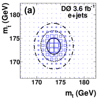
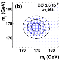
The final likelihood for $\Delta$ is constructed by marginalizing $M_{\mbox{\scriptsize\,sum}}$ with a flat prior and subsequently combining $e$+jets and $\mu$+jets channels.

Compared to an M${}_{\mbox{\scriptsize\,t}}$ estimate, importance of various sources of systematic uncertainties is substantially different in the $\Delta$ measurement. For example, the jet energy scale-related uncertainty of a few percent becomes relatively insignificant, while effects which can have different impact upon reconstruction of $t$ vs. $\bar{t}$ decay products become of major concern. Such effects include the mismeasurement of the lepton charge and uncertainties from modeling differences in the response of the calorimeter to $b$ and $\bar{b}$ jets (most notably, a different content of $K^{+}/K^{-}$ mesons which have different interaction cross sections with the calorimeter material). Taking these considerations into account, the DØ collaboration obtains an estimate $\Delta=0.8\pm 1.8\,(\mbox{stat.})\pm 0.5\,(\mbox{syst.})$ GeV/$c^{2}$, consistent with ${\it M}_{\mbox{\scriptsize\,t}}={\it M}_{\,\bar{\mbox{\scriptsize t}}}$.

The CDF measurement of $\Delta$ utilized 5.6 fb${}^{\mbox{\scriptsize-1}}$ of Run II data [197]. This measurement is also performed in the $\ell$+jets channel, with the sample selection criteria similar to those used for the CDF M${}_{\mbox{\scriptsize\,t}}$ measurement described in Section 7.1. Events without $b$ tags are admitted as well, with an additional requirement $H_{T}>250$ GeV. The template approach is utilized. The event-by-event estimate of $\Delta$, $\Delta m_{t}$, is obtained from a kinematic fit. $\chi^{2}$ is evaluated according to expression (2) in which the two terms that include $m_{t}$ are replaced by $(M_{b\ell\nu}-(M_{\mbox{\scriptsize\,sum}}-dm_{reco}/2))^{2}/\Gamma_{t}^{2}+(M_{bjj}-(M_{\mbox{\scriptsize\,sum}}+dm_{reco}/2))^{2}/\Gamma_{t}^{2}$. $M_{\mbox{\scriptsize\,sum}}$ is fixed at 172.5 GeV/$c^{2}$. $\Delta m_{t}$ is subsequently defined by $\Delta m_{t}=-Q_{\ell}\cdot dm_{reco}^{min}$, where $Q_{\ell}$ is the sign of the lepton charge which distinguishes $t$ and $\bar{t}$, and $dm_{reco}^{min}$ is the value of $dm_{reco}$ that minimizes the $\chi^{2}$. Two-dimensional templates are constructed using the two $\Delta m_{t}$ values which correspond to the best and second best (over distinct jet-to-parton assignments and kinematic solutions) values of $\chi^{2}$, with input $\Delta$ varied between $-20$ and 20 GeV/$c^{2}$. To improve the template modeling, the event sample is split into six subsamples with zero, one, or two $b$ tags and different values of $Q_{\ell}$. Templates are subsequently fitted to the distributions of best and second best $\Delta m_{t}$ observed in the data. To determine $\Delta$, log-likelihoods from all event subsamples are added and the statistical uncertainty is scaled by 1.04 to ensure proper frequentist coverage (the bias is found to be consistent with zero).

As in the DØ measurement, the dominant part of the systematic uncertainty is due to signal mismodeling. CDF obtains $\Delta=-3.3\pm 1.4\,(\mbox{stat.})\pm 1.0\,(\mbox{syst.})$ GeV/$c^{2}$, which is consistent with ${\it M}_{\mbox{\scriptsize\,t}}={\it M}_{\,\bar{\mbox{\scriptsize t}}}$ at the about $2\sigma$ level.

7.7 Mass from cross section

The theoretical $t\bar{t}$ cross section prediction depends on the top mass, as shown in Figure 4 in Section 2.1. Therefore, given a theory curve and a cross section measurement, it is possible to extract a top mass estimate. This has been done by the DØ collaboration using several cross section measurements: in the dilepton channel [198], using a combination of different channels [199], and, most recently, in the $\ell$+jets channel [13]. The latter measurement, compared with two theoretical cross section calculations, is shown in Figure 34.

Figure 34: Top cross section vs. top quark mass as calculated by different authors [11, 200]. The data point is the DØ  measurement [13] mentioned in the text.

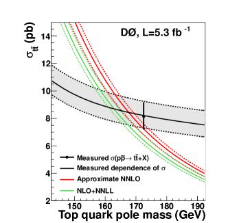
The measured value of the cross section is positioned at ${\it M}_{\mbox{\scriptsize\,t}}$ = 172.5 GeV/$c^{2}$, the mass value used to calculate the acceptance for the measurement. The gray band depicts the total experimental uncertainty plotted as a function of the top mass. The appoximate NNLO calculations are from Ref [11], the NLO+NNLL calculations are from Ref [200]. The uncertainties in the theoretical calculations are shown by the dotted lines. The analysis extracting the top mass estimate from these cross section approximations makes the assumption that $M_{\mbox{\scriptsize\,MC}}$ = $M_{\mbox{\scriptsize\,pole}}$ (see Section 1.1). The results are:

$M_{\mbox{\scriptsize\,pole}}=163.0^{+5.4}_{-4.0}$ GeV/$c^{2}$ for NLO+NNLL

$M_{\mbox{\scriptsize\,pole}}=167.5^{+5.4}_{-4.9}$ GeV/$c^{2}$ for approx. NNLO

The value obtained with the approximate NNLO calculation is closer to the top mass measured directly but the uncertainties are large in both cases. DØ has also extracted a value for the top quark mass in the $\overline{MS}$ renormalization scheme, as mentioned in Section 1.1.

8 Combination

While all individual M${}_{\mbox{\scriptsize\,t}}$ measurements provide important information per se, a more precise estimate can still be obtained by combining the results. Such a combination is regularly performed by the Tevatron Electroweak Working Group (TEVEWWG) [201]. Normally, the current most precise measurement in each decay mode per experiment is selected to enter into the Tevatron combination. Utilizing measurements which use overlapping datasets requires the estimation of the statistical correlations among the measurements themselves. Many systematic uncertainties are correlated among channels as their sources affect either the modeling of the signal and/or background events or the calibration of the detector response to the final state objects. These correlations have to be understood in detail in order to combine the measurements properly. This necessitates a collaborative effort by the authors of the M${}_{\mbox{\scriptsize\,t}}$ measurements that are being combined.

8.1 Method and general issues

The CDF and DØ collaborations use the best linear unbiased estimator (BLUE) method [144, 145] to combine their measurements. The collaborations have been working jointly for a number of years with the purpose of understanding the sources of the systematic uncertainty and their interdependence. Once an independent uncertainty source is identified, its impact on the M${}_{\mbox{\scriptsize\,t}}$ measurements is evaluated by assigning a correlation matrix which has an entry for each pair of results. Before the final combination is performed, systematic sources are collected into groups that share similar physical origins and whose impact on the measurements is described by the same correlation matrix. This grouping is described below:

Statistics

. The statistical uncertainty associated with the M${}_{\mbox{\scriptsize\,t}}$ determination.

iJES

: Part of the JES uncertainty which originates from in situ calibration procedures that use the $W$ boson mass in decay modes with at least one hadronically decaying $W$.

aJES

: Part of the JES uncertainty which originates from the difference in calorimeter electromagnetic over hadronic ($e/h$) response for $b$ jets and light-quark jets.

bJES

: Part of the JES uncertainty which originates from generator modeling of $b$ jets. For both CDF and DØ, it includes the uncertainties arising from variations in the semileptonic branching fractions, $b$ fragmentation functions, and differences in the color flow between $b$ jets and light-quark jets.

cJES

: Part of the JES uncertainty which originates from the modeling of light-quark fragmentation and out-of-cone corrections. For DØ Run II measurements, it is included in the dJES category.

dJES

: Part of the JES uncertainty which originates from the finite size of the data samples used to calibrate the jet energy response of the detectors. This includes uncertainties associated with the $\eta$-dependent JES corrections which are estimated using dijet data events. For DØ this also includes the uncertainties in the light jet response and uncertainties that arise due to the sample dependence of jet corrections derived with the $\gamma$+jets data.

rJES

: The remaining part of the JES uncertainty. For CDF, this is dominated by uncertainties in the calorimeter response to light-quark jets, and also includes small uncertainties associated with the multiple interaction and underlying event corrections. For DØ Run II measurements, uncertainty sources of this kind belong to the dJES category.

LepPt

: The systematic uncertainty related to the calibration of lepton transverse momentum measurements.

Signal

: The systematic uncertainty arising from uncertainties in the $t\bar{t}$ modeling. This is obtained summing in quadrature several different sources. It includes uncertainties in the ISR and FSR descriptions; the uncertainty on the knowledge of the PDFs; the systematic uncertainty arising from a variation of the phenomenological description of color reconnection between final state particles. The systematic uncertainty associated with variations of the physics model used to calibrate the data analysis methods, correlated across all measurements. It includes variations observed when ISAJET (Run I) or HERWIG or ALPGEN+PYTHIA are substituted to PYTHIA in modeling the $t\bar{t}$ signal. For DØ it also includes the uncertainty that arises from considering or ignoring higher order Feynman diagrams.

Detector modeling (DetMod)

: Uncertainty in the modeling of the detector in the MC simulation, such as the uncertainty on the jet energy resolution and identification efficiency.

Background from MC (BGMC)

: Uncertainty in the background modeling, including sample composition and shape of relevant distributions, including the choice of the factorization scale used to model $W$+jets production.

Background from data (BGData)

: This group includes uncertainties associated with the modeling of the QCD multijet background in the all-hadronic, ${\not}{E_{T}}$+jets and $\ell$+jets channels, uncertainties associated with the modeling of the Drell-Yan background in the dilepton channel

Method

: The systematic uncertainty arising from any source specific to a particular data analysis method, including the finite Monte Carlo statistics available for method calibration.

Uranium Noise and Multiple Interactions (UN/MI)

: This is specific to DØ and includes the uncertainty arising from uranium noise in the DØ calorimeter and from the multiple interaction corrections to the JES. For DØ Run I these uncertainties were sizable, while for Run II, owing to the shorter calorimeter electronics integration time and in situ JES calibration, these uncertainties are negligible.

Multiple Hadron Interactions (MHI)

: The systematic uncertainty arising from the mismodeling of the distribution of the number of collisions per Tevatron bunch crossing.

Reasonable variations in the assignment of uncertainty sources to these groups, in the back-propagation of the bJES uncertainties to Run I measurements, and in the assumed magnitude of the correlations have produced a negligible impact on the combined M${}_{\mbox{\scriptsize\,t}}$ measurement and its total uncertainty.

8.2 Latest combination

The latest Tevatron combination [202] utilizes twelve different measurements of M${}_{\mbox{\scriptsize\,t}}$. These are the Run I and Run II CDF measurements in the $\ell$+jets (l+j in the summary table) [100, 149], all-hadronic (all-j) [181, 113], and dilepton (di-l) [102, 203] channels, the DØ Run I and Run II measurements in the $\ell$+jets [104, 204] and dilepton [127, 193] channels, one CDF measurement in the $\ell$+jets channel that used tracking information with minimal dependence on the jet response (trk) [122], and one CDF measurement performed in the ${\not}{E_{T}}$+jets signature [118]. All these measurements are summarized in Table 10 together with their uncertainties.

Table 10: Summary of the measurements used to determine the Tevatron average M${}_{\mbox{\scriptsize\,t}}$. Integrated luminosity ($\int\mathcal{L}\;dt$) has units in fb^-1, and all other numbers are in GeV$/c^{2}$. The uncertainty categories and their correlations are described in the Sec. 8.1. The total systematic uncertainty and the total uncertainty are obtained by adding the relevant contributions in quadrature. “n/a” stands for “not applicable”,“n/e” for “not evaluated”.

	Run I published					Run II published					Run II prel.
	CDF			DØ		CDF			DØ		CDF		Tevatron
	allh	l+jt	di-l	l+jt	di-l	di-l	Lxy	l+jt	di-l	l+jt	allh	MEt	all
$\int\mathcal{L}\;dt$	0.1	0.1	0.1	0.1	0.1	5.6	1.9	5.6	5.2	3.6	5.8	5.7	$\leq$ 5.8
Result	186.0	176.1	167.4	180.1	168.4	170.28	166.90	173.00	173.97	174.94	172.47	172.32	173.18
iJES	n/a	n/a	n/a	n/a	n/a	n/a	n/a	0.58	n/a	0.53	0.95	1.54	0.39
aJES	n/a	n/a	n/a	0.0	0.0	0.14	n/a	0.13	1.57	0.0	0.03	0.12	0.09
bJES	0.6	0.6	0.8	0.7	0.7	0.33	n/a	0.23	0.40	0.07	0.15	0.26	0.15
cJES	3.0	2.7	2.6	2.0	2.0	2.13	0.36	0.27	n/a	n/a	0.24	0.20	0.05
dJES	0.3	0.7	0.6	n/a	n/a	0.58	0.06	0.01	1.50	0.63	0.04	0.05	0.20
rJES	4.0	3.4	2.7	2.5	1.1	2.01	0.24	0.41	n/a	n/a	0.38	0.45	0.12
LepPt	n/e	n/e	n/e	n/e	n/e	0.27	n/a	0.14	0.49	0.18	-	-	0.10
Signal	2.0	2.6	2.9	1.1	1.8	0.73	0.90	0.56	0.74	0.77	0.62	0.74	0.51
DetMod	0.0	0.0	0.0	0.0	0.0	0.0	0.0	0.0	0.33	0.36	0.0	0.0	0.10
UN/MI	n/a	n/a	n/a	1.3	1.3	n/a	n/a	n/a	n/a	n/a	n/a	n/a	0.00
BGMC	1.7	1.3	0.3	1.0	1.1	0.24	0.80	0.27	0.0	0.18	0.0	0.0	0.14
BGData	0.0	0.0	0.0	0.0	0.0	0.14	0.20	0.06	0.47	0.23	0.56	0.12	0.11
Method	0.6	0.0	0.7	0.6	1.1	0.12	2.50	0.10	0.10	0.16	0.38	0.14	0.09
MHI	n/e	n/e	n/e	n/e	n/e	0.23	0.0	0.10	0.0	0.05	0.08	0.16	0.08
Syst	5.7	5.3	4.9	3.9	3.6	3.13	2.82	1.06	2.45	1.24	1.40	1.82	0.75
Stat	10.0	5.1	10.3	3.6	12.3	1.95	9.00	0.65	1.83	0.83	1.43	1.80	0.56
Total	11.5	7.3	11.4	5.3	12.8	3.69	9.43	1.23	3.06	1.50	2.00	2.56	0.94

All Run I measurements have relatively large statistical uncertainties due to the limited size of the $t\bar{t}$ samples collected. Their systematic uncertainties are dominated by the total jet energy scale (JES) uncertainty. In Run II, both CDF and DØ take advantage of the larger $t\bar{t}$ samples available and employ new analysis techniques to reduce both of these uncertainties.

The statistical uncertainty is uncorrelated among the measurements due to the non-overlapping event samples used. The only possible exception to this rule is the CDF Run II M${}_{\mbox{\scriptsize\,t}}$ measurements in the $\ell$+jets channel named “l+j” and “trk” in the Table 10 caption. The latter employs a subset of the data sample used by the former. The statistical correlation between the trk analysis and an older Run II CDF l+j measurement was studied using Monte Carlo signal-plus-background pseudo-experiments which correctly accounted for the sample overlap and was found to be consistent with zero. The statistical part of the JES systematic uncertainty (iJES) is also uncorrelated, for the same reasons. The correlation matrices for the statistical uncertainty and for the iJES category are thus the trivial unit matrices. Unit matrix is also used to represent correlations for the Method category.

The correlation among the measurements for the bJES, cJES, and Signal uncertainties is taken to be 100%. The uncertainties in the aJES, dJES, LepPt, MHI, DetMod and BGData categories are taken to be 100% correlated among all Run I and all Run II measurements within the same experiment, but uncorrelated between Run I and Run II, and uncorrelated between the experiments. The uncertainties in the rJES and UN/MI categories are taken to be 100% correlated among all measurements within the same experiment but uncorrelated between the experiments. The uncertainty in the BGMC category is taken to be 100% correlated among all measurements in the same channel and among experiments.

The combined value of the top quark mass is ${\it M}_{\mbox{\scriptsize\,t}}=173.18\pm 0.56\,(\mbox{stat.})\pm 0.75\,(\mbox{syst.})$ GeV/$c^{2}$. The $\chi^{2}$ value of this result is 8.3 for 11 degrees of freedom. The corresponding confidence level is 68%, indicating good agreement among the input measurements. Adding the statistical and systematic uncertainties in quadrature yields a total uncertainty of 0.94 GeV/$c^{2}$, corresponding to a relative precision of 0.54% on the top quark mass. Rounded off to two significant digits in the uncertainty, the combined result is ${\it M}_{\mbox{\scriptsize\,t}}=173.2\pm 0.9$ GeV/c².

The input measurements and the current combination are displayed in Figure 35.

Figure 35: Summary of the input measurements and resulting Tevatron average mass of the top quark [202].

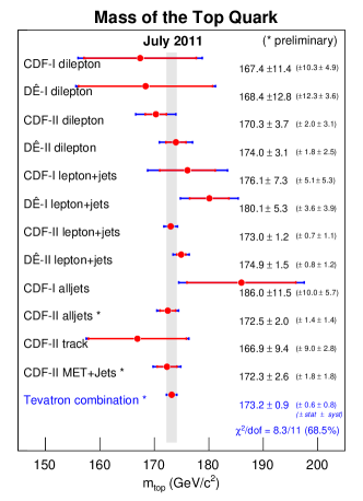
The most recent CDF and DØ measurements in the $\ell$+jets channel which use the matrix element method enter the combination with the largest weights, followed by the CDF template measurement in the all-hadronic channel.

It can be deduced from Table 10 that the total JES-related uncertainty is $0.49$ GeV/$c^{2}$, with $0.39$ GeV/$c^{2}$ coming from the statistical component and $0.30$ GeV/$c^{2}$ from other sources. As the most significant fraction of the JES uncertainty is still statistical in nature, the M${}_{\mbox{\scriptsize\,t}}$ precision can be further improved by simply analyzing larger collision datasets already collected by CDF and DØ.

When the complete dataset produced by the Tevatron will be analyzed, the total uncertainty of the M${}_{\mbox{\scriptsize\,t}}$ determination will likely drop around $0.8$ GeV/$c^{2}$, even without further understanding of the systematic sources. By the time Tevatron operations will close at the end of 2011, LHC will have produced much larger $t\bar{t}$ samples, so the expected M${}_{\mbox{\scriptsize\,t}}$ statistical uncertainty will soon be negligible. It will be important to establish the correlations among the measurements performed at the Tevatron and at the LHC so that one single estimate of the top quark mass can still be provided to the particle physics community.

9 Conclusions

From the first direct observation of top quark pair production and throughout the whole lifetime of the Tevatron collider program, precision determination of the top quark mass has been the subject of intensive studies at the CDF and DØ experiments. A number of sophisticated M${}_{\mbox{\scriptsize\,t}}$ measurement techniques have been developed. Important methodological advances include the first practical application of the matrix element analysis method to hadron collider data and introduction of the in situ jet energy scale calibration with the $W$ boson mass. These particular improvements led to a substantial reduction in the statistical and systematic uncertainty, respectively. Recent M${}_{\mbox{\scriptsize\,t}}$ measurements performed in different final states of the $t\bar{t}$ system, with multiple analysis methods and with independent experimental setups are all in close agreement with each other, in accordance with Standard Model expectations.

The current combined estimate of the top quark mass by CDF and DØ is

$${\it M}_{\mbox{\scriptsize\,t}} =173.18\pm 0.56\,(\mbox{stat.})\pm 0.75\,(\mbox{syst.})\,\,\mbox{GeV}/c^{2}$$

$$=173.18\pm 0.94\,(\mbox{total})\,\,\mbox{GeV}/c^{2}$$

Its accuracy is limited by systematic uncertainties resulting from a number of imprecisely known calibration parameters, both theoretical and experimental. Although the knowledge of some of these parameters will automatically improve as more data becomes available, further reduction of the uncertainty will require more detailed understanding of the underlying physics processes. Whenever possible, this understanding should be translated into the calculation of the corresponding systematic uncertainty on event-by-event basis. Modeling of parton showering and hadronization, together with accurate representation of nonlinearities in the detector jet response, will remain critical for CDF and DØ.

In the future, when much larger $t\bar{t}$ samples are accumulated by the LHC experiments, M${}_{\mbox{\scriptsize\,t}}$ measurements which do not use jets could outperform more conventional techniques. The ultimate precision will be reached by scanning the $t\bar{t}$ center-of-mass energy production threshold at a high energy lepton collider.

10 Acknowledgments

We thank Christian Bauer for guidance regarding the relationship between the experimental and theoretical top quark mass. We are also indebted to Paul Lujan, Jeremy Lys, Yvonne Peters, and Elizaveta Shabalina for reading the manuscript and providing useful comments.

References

- [1] Bhattacharyya G 2011 A pedagocal review of electroweak symmetry breaking scenarios Rep. Prog. Phys.74 026201
- [2] Quigg C Top-ology, 2010, TASI lectures arXiv:hep-ph/9704332
- [3] ALEPH DELPHI L3 OPAL SLD CDF DØ Coll., the LEP Tevatron SLD Electroweak Working Group 2010 CERN-PH-EP-2010-095
- [4] Innes W et al. 1977 Phys. Rev. Lett. 39 252
- [5] CDF Coll., Abe F et al. 1995 Phys. Rev. Lett. 74 2626
- [6] DØ Coll., Abachi S et al. 1995 Phys. Rev. Lett. 74 2632
- [7] CDF Coll., Abe F et al. 1994 Phys. Rev. D 50 2966
- [8] Nakamura K et al Review of Particle Physics J. Phys. G: Nucl. Part. Phys. 37 p. for q mass
- [9] Bardeen W A, Hill C T, and Lindner M 1990 Phys. Rev. D 41 1647
- [10] Hill C T 1991 Phys. Lett. B 266 419 Hill C T 1995 Phys. Lett. B 345 483
- [11] Langenfeld U Moch S and Uwer P 2009 Phys. Rev. 80 054009.
- [12] Hoang A H Stewart J W 2008 Nuclear Phys. Proc. Suppl. 185 220 (arXiv:0808.0222v1)
- [13] DØ Coll., Abazov V M 2011 Submitted to Phys. Rev. Lett. arXiv:1104.2887v1
- [14] Hoang A H et al. 2008 Phys. Rev. Lett. 101 15602 (arXiv:0803.4214v2)
- [15] Smith M C Willenbrock S S 1997 Phys. Rev. Lett. 79 3825
- [16] Buckley A et al 2011 arXiv:1101.2599v1 Submitted to Physics Reports
- [17] Sjostrand T et al 2001 Comput. Phys. Commun. 135 238
- [18] Fleming S et al 2008 Phys. Rev. D 77 074010 (arXiv:hep-ph/0703207) Fleming S et al 2008 Phys. Rev. D 77 114003 (arXiv:0711.2099)
- [19] Cacciari M et al. 2004 JHEP 0404 068
- [20] Kidonakis N and Vogt R 2003 Phys. Rev. D 68 114014 Berger E L and Contopanagos H, 1995 Phys. Lett. B 361 115 Bernreuther W al 2004 Nucl. Phys. B 690 81
- [21] CDF Coll., Aaltonen T et al. 2009 CDF CONF Note 9913
- [22] Cacciari M et al 2008 JHEP 09 127 (arXiv:0804.2800)
- [23] Kidonakis N and Vogt R 2008 Phys. Rev. 78 074005 (arXiv:0805.3844)
- [24] CDF Coll., Aaltonen T et al. 2010 Phys. Rev. Lett. 105 012001 [arXiv:1004.3224 [hep-ex]].
- [25] Deliot F Glenzinski A D 2010 Top Quark Physics at the Tevatron, Submitted to Rev. of Mod. Phys. (arXiv:1010.1202v1)
- [26] Wicke D 2010 Properties of the Top Quark Submittted to EPJ (arXiv:1005.2460)
- [27] CDF Coll., Aaltonen T et al. Phys. Rev. D 83 (2011) 031104 [arXiv:1012.3093 [hep-ex]].
- [28] DØ Coll., Abazov V M et al. arXiv:1103.1871 [hep-ex].
- [29] CDF Coll., Aaltonen T et al 2008 Phys. Rev.D 78 111101 arXiv:0712.3273.
- [30] CDF Coll., Aaltonen T et al. 2009 Phys. Rev. Lett. 102, 222003;
- [31] DØ Coll., Abazov V M et al. 2010 “Dependence of the production cross section on the transfer momentum of the top quark” Phys. Lett. B 693 515
- [32] CDF Coll., Aaltonen et al 2011 Phys. Rev.D 83 112003 (arXiv:11010034)
- [33] DØ Coll., Abazov V M et al 2010 CONF Note 6062
- [34] Nason P Dawson S and Ellis R K 1988 Nucl. Phys.B 303 607 and 1989 Nucl. Phys.B 327 49 and 1990 (E) B 335 260 Beenakker W et al 1989 Phys. Rev.D 40 54 and 1991 Nucl. Phys.B 351 507
- [35] Kidonakis N 2011 arXiv:1105.5167
- [36] CDF Coll., Acosta D E et al. 2005 Phys. Rev. Lett. 95, 102002 [arXiv:hep-ex/0505091]
- [37] DØ Coll., Abazov V M et al. 2008 Phys. Rev. Lett. 100 192003 [arXiv:0801.1326 [hep-ex]]
- [38] CDF Coll., Aaltonen T et al. 2009 Phys. Lett. B 674 160 [arXiv:0811.0344 [hep-ex]]
- [39] DØ Coll., Abazov V M et al. 2011 Phys. Rev. D 83 032009 [arXiv:1011.6549 [hep-ex]]
- [40] CDF Coll., Aaltonen T et al. 2010 Phys. Rev. Lett. 105 101801 [arXiv:1006.4597 [hep-ex]]
- [41] CDF Coll., Aaltonen T et al. 2010 Phys. Rev. Lett. 105, 232003 [arXiv:1008.3891 [hep-ex]]
- [42] DØ Coll., Abazov V M et al. 2011 Phys. Rev. Lett. 106 022001 [arXiv:1009.5686 [hep-ex]]
- [43] CDF Coll., Acosta D et al 2005 Phys. Rev.D 72 052003 Sill A 2000 “CDF RunII Silicon tracking project” Nucl. Instrum. MethodsA 447 1
- [44] CDF Coll., Aaltonen T et al 2011 Measurement of Properties of f0(980) Decay at CDF [arXiv:1106.3682] Submitted to Phys. Rev.D
- [45] CDF Coll., Abe F et al. 1992 Phys. Rev. Lett. 68 1104
- [46] DØ Coll., Abazov V M et al. Public page: http://www-d0.fnal.gov/phys_id/jes/public_RunIIa/
- [47] DØ Coll., Abazov V M et al. 2006 “The Upgraded DØ Detector” Nucl. Instrum. MethodsA 565 463
- [48] DØ Coll., Abazov V M et al 2007 Phys. Rev.D 76, 052006.
- [49] DØ Coll., Abazov V M et al 2007 Phys. Rev.D 76, 092007.
- [50] Blazey et al. 2000 Proceedings of the Physics at Run II:QCD and Weak Boson Physics Workshop Batavia Illinois, 4-6 Nov 1999 FERMILAB-CONF-00-092-E (Hep-ex/0005012)
- [51] Cheng Y 1995 IEEE Trans. Patt. Analysis and Mach. Intelligence 17 790-9
- [52] Ellis S D, Huston J and Tonnesman M arXiv:hep-ph/0111434v1. Ellis S D et al. 2008 Jets in hadron-hadron collisions Progress in Particle and Nuclear Physics 50 484-551
- [53] Volobouev I 2011 J. Phys.: Conf. Ser 293 012028
- [54] Gringhammer G, Rudowitz M and Peters S Nucl. Instrum. MethodsA 290 469
- [55] Brun R, Hagelberg R, Hansroul M and Lassalle J C, CERN-DD-78-2-REV. CERN Program Library Long Writeup Report No. W5013, 1993.
- [56] Bhatti A et al. 2006 “Determination of the Jet Energy Scale at the Collider Detector at Fermilab” Nucl. Instrum. MethodsA 566 375 [arXiv:hep-ex/0510047v1]
- [57] Voutilainen M 2008 Measurement of the inclusive jet cross section at DØ PHD Thesis: FERMILAB-THESIS-2008-x
- [58] DØ Coll., Abazov V M et al. 2008 Phys. Rev. Lett. 101, 062001. [arXiv:0802.2400 [hep-ex].
- [59] DØ Coll., Abazov V et al. 2007 Phys. Rev.D 75 092001
- [60] DØ Coll., Abazov V M et al. 2010 “b-jet identification in the DØ experiment” Nucl. Instrum. MethodsA 620 490
- [61] CDF Coll., Acosta D et al. 2005 Phys. Rev.D 71 052003.
- [62] CDF Coll., Acosta D et al. 2004 http://www-cdf.fnal.gov/physics/new/top/2004/btag/
- [63] CDF Coll., Aaltonen T et al. 2010 CDF-CONF-10049
- [64] DØ Coll., Abazov V M et al. 2006 Phys. Rev.D 74 112004
- [65] CDF Coll., Aaltonen T et al. 2011 Phys. Rev.D 83 111101 Preprint arXiv:1105.0192v3 [hep-ex] Hyunsu Lee University of Chicago private comunication
- [66] DØ Coll., Abazov V et al. 2010 Preprint arXiv:1105.0320v1 [hep-ex]
- [67] CDF Coll., Aaltonen T et al. 2008 Phys. Rev.D 77 0111108
- [68] DØ Coll., Abazov V M et al. 2011 Submitted to Phys. Rev.D[arXiv:1101.0124 [hep-ex]]
- [69] Marchesini G et al. 1992 Comput. Phys. Commun. 67 465-508
- [70] Gribov V N and Lipatov L N 1972 Sov. J. Nucl. Phys. 15, 438 [Yad. Fiz. 15, 781].
- [71] Altarelli G and Parisi G 1977 Nucl. Phys. B 126, 298.
- [72] Dokshitzer Y L 1977 Sov. Phys. JETP 46 641 [Zh. Eksp. Teor. Fiz. 73 1216].
- [73] Jadach S, Was Z, Decker E and Kuhn J H 1993 Comput. Phys. Commun. 76, 361.
- [74] Lange D J 2001 Nucl. Instrum. Meth. A 462, 152.
- [75] Mangano M L, Moretti M, Piccinini F, Pittau R and Polosa A D 2003 JHEP 0307 001 [arXiv:hep-ph/0206293].
- [76] Alwall J et al. 2007 JHEP 0709, 028 [arXiv:0706.2334 [hep-ph]].
- [77] Mangano M L, Moretti M, Piccinini F and Treccani M 2007 JHEP 0701, 013 [arXiv:hep-ph/0611129].
- [78] Frixione S and Webber B R 2006 arXiv:hep-ph/0612272.
- [79] Field R 2005 FERMILAB-CONF-06-408-E, FNAL.
- [80] CDF Coll., Field R and Group R C 2005 arXiv:hep-ph/0510198.
- [81] Skands P Z 2009 arXiv:0905.3418 [hep-ph].
- [82] CTEQ Coll., Lai H L et al. 2000 Eur. Phys. J. C 12, 375 [arXiv:hep-ph/9903282].
- [83] Pumplin J, Stump D R, Huston J, Lai H L, Nadolsky P M and Tung W K 2002 JHEP 0207, 012 [arXiv:hep-ph/0201195].
- [84] Martin A D, Roberts R G, Stirling W J and Thorne R S 1998 Eur. Phys. J. C 4 463 [arXiv:hep-ph/9803445].
- [85] CDF Coll., Aaltonen T et al. 2010 Phys. Rev. D 82 052002 [arXiv:1002.2919 [hep-ex]].
- [86] DØ Coll., Abazov V M et al. 2009 Phys. Lett. B 679 177S200 [arXiv:0901.2137 [hep-ex]].
- [87] CDF Coll., Aaltonen T et al. 2010 Phys. Rev.D81, 052011 [arXiv:1002.0365 [hep-ex]].
- [88] DØ Coll., Abazov V M et al. 2010 Phys. Rev. D 82, 032002 [arXiv:0911.4286 [hep-ex]].
- [89] CDF Coll., Aaltonen T et al. 2011 arXiv:1105.1806 [hep-ex].
- [90] Lujan P 2009 Precision Measurement of the Top Quark Mass in the Lepton + Jets Channel Using a Matrix Element Method with Quasi-Monte Carlo Integration FERMILAB-THESIS-2009-26
- [91] Campbell J M and Ellis R K 2002 Phys. Rev. D 65 113007 [arXiv:hep-ph/0202176].
- [92] CompHEP Coll., Boos E et al. 2004 Nucl. Instrum. Meth. A 534, 250 [arXiv:hep-ph/0403113].
- [93] CDF Coll., Aaltonen T et al. 2009 Phys. Rev.D 79 092005
- [94] CDF Coll., Aaltonen T et al. 2009 CDF Conf. Note 9679
- [95] James F 2006 Statistical Methods in Experimental Physics (Singapore: World Scientific)
- [96] DØ Coll., Abazov V et al. 2004 Nature 429 638-42
- [97] DØ Coll., Abazov V et al. 2006 Phys. Rev.D 74 092005
- [98] DØ Coll., Abazov V et al. 2008 Phys. Rev. Lett. 101 182001
- [99] DØ Coll., Abazov V et al. 2011 Preprint Submitted to Phys. Rev.DarXiv:1105.6287v1 [hep-ex]
- [100] CDF Coll., Abe F et al. 1998 Phys. Rev. Lett. 80 2767-72
- [101] DØ Coll., Abachi S et al. 1997 Phys. Rev. Lett. 79 1197-1202
- [102] CDF Coll., Abe F et al. 1999 Phys. Rev. Lett. 82 271-6
- [103] CDF Coll., Affolder T et al. 2001 Phys. Rev.D 63 032003
- [104] DØ Coll., Abbott B et al. 1998 Phys. Rev.D 58 052001
- [105] CDF Coll., Aaltonen T et al. 2007 Phys. Rev.D 76 072009
- [106] DØ Coll., Abazov V et al. 2005 Phys. Lett.B 606 25-33
- [107] CDF Coll., Abulencia A et al. 2006 Phys. Rev.D 73 112006
- [108] CDF Coll., Aaltonen T et al. 2009 Phys. Rev.D 79 072005
- [109] DØ Coll., Abazov V et al. 2007 DØ Conf. Note 5463
- [110] DØ Coll., Abazov V et al. 2007 Phys. Lett.B 655 7-14
- [111] CDF Coll., Aaltonen T et al. 2008 Phys. Rev. Lett. 100 062005
- [112] DØ Coll., Abazov V et al. 2009 Phys. Rev.D 80 092006
- [113] CDF Coll., Aaltonen T et al. 2011 CDF Conf. Note 10456
- [114] CDF Coll., Abulencia A et al. 2006 Phys. Rev.D 73 032003
- [115] CDF Coll., Aaltonen T et al. 2010 Phys. Rev.D 81 031102(R)
- [116] CDF Coll., Abulencia A et al. 2006 Phys. Rev. Lett. 96 022004
- [117] CDF Coll., Aaltonen T et al. 2009 Phys. Rev.D 79 072010
- [118] CDF Coll., Aaltonen T et al. 2011 Preprint Submitted to Phys. Rev. Lett.arXiv:0910.0969v1 [hep-ex]
- [119] CDF Coll., Acosta D et al. 2004 CDF Conf. Note 7102
- [120] CDF Coll., Abe F et al. 1998 Phys. Rev. Lett. 80 2779-84
- [121] CDF Coll., Abulencia A et al. 2007 Phys. Rev.D 75 071102(R)
- [122] CDF Coll., Aaltonen T et al. 2010 Phys. Rev.D 81 032002 arXiv:0910.0969v1 [hep-ex]
- [123] CDF Coll., Abulencia A et al. 2007 CDF Conf. Note 8959
- [124] CDF Coll., Aaltonen T et al. 2009 CDF Conf. Note 9831
- [125] CDF Coll., Aaltonen T et al. 2011 Phys. Lett.B 698 371-9
- [126] CDF Coll., Aaltonen T et al. 2009 Phys. Rev.D 80 051104(R)
- [127] DØ Coll., Abbott B et al. 1998 Phys. Rev. Lett. 80 2063-68
- [128] DØ Coll., Abbott B et al. 1999 Phys. Rev.D 60 052001
- [129] Scott D 1992 Multivariate Density Estimation: Theory, Practice, and Visualization (Wiley)
- [130] James F 1994 CERN Program Library Long Writeup D506
- [131] Fan J and Gijbels I 1996 (London: Chapman and Hall/CRC)
- [132] Berger J, Liseo B and Wolpert R 1999 Stat. Science 14 1-28
- [133] Bhat P, Prosper H and Snyder S 1997 Phys. Lett.B 407 73-78
- [134] CDF Coll., Aaltonen T et al. 2007 Phys. Rev. Lett. 98, 142001 [hep-ex/0612026].
- [135] CDF Coll., Aaltonen T et al. 2008 CDF Conf. Note 9265
- [136] DØ Coll., Abazov V et al. 2004 DØ Conf. Note 4574
- [137] Punzi G 2004 Preprint arXiv:physics/0401045v1
- [138] DØ Coll., Abazov V et al. 2009 Phys. Lett.B 679 177-185
- [139] DØ Coll., Abazov V et al. 2011 Preprint arXiv:1104.2887v1 [hep-ex]
- [140] CDF Coll., Aaltonen T et al. 2007 CDF Conf. Note 8669
- [141] Kopylov G 1970 Fundamentals of the Kinematics of Resonances (in Russian) (Moscow: Nauka) p 429-442
- [142] DØ Coll., Abazov V et al. 2010 D0 Conf. Note 6104
- [143] Dalitz R and Goldstein G 1992 Phys. Rev.D 45 1531-43
- [144] Lyons L, Gibaut D and P. Clifford 1988 Nucl. Instrum. Meth. A270 110;
- [145] Valassi A 2003 Nucl. Instrum. Meth. A500 391;
- [146] Volobouev I 2011 Preprint arXiv:1101.2259v1 [physics.data-an]
- [147] Artoisenet P, Lemaitre V, Maltoni F and Mattelaer O 2010 J. High Energy Phys. JHEP12(2010)068
- [148] CDF Coll., Aaltonen T et al. 2009 Phys. Rev.D 79 072001
- [149] CDF Coll., Aaltonen T et al. 2010 Phys. Rev. Lett. 105 252001
- [150] CDF Coll., Aaltonen T et al. 2009 CDF Conf. Note 9725
- [151] CDF Coll., Abulencia A et al. 2006 Phys. Rev.D 74 032009
- [152] CDF Coll., Abulencia A et al. 2007 Phys. Rev.D 75 031105(R)
- [153] Lepage G 1978 J. of Comput. Phys. 27 192-203
- [154] Niederreiter H 1992 Random Number Generation and Quasi-Monte Carlo Methods (SIAM)
- [155] Kondo K 1988 J. Phys. Soc. Japan 57 4126-40
- [156] Kondo K 2005 Preprint arXiv:hep-ex/0508035v2
- [157] CDF Coll., Abulencia A et al. 2006 Phys. Rev.D 73 092002
- [158] CDF Coll., Aaltonen T et al. 2007 CDF Conf. Note 9135
- [159] Tsuchiya R 2006 Measurement of the Top Quark Mass by Dynamical Likelihood Method using the Dilepton Events with the Collider Detector at Fermilab FERMILAB-THESIS-2006-69
- [160] CDF Coll., Aaltonen T et al. 2009 Phys. Rev. Lett. 102 152001
- [161] Barlow R 1999 MAN/HEP/99/4
- [162] CDF Coll., Blair R et al. 2001 FERMILAB-Pub-96/390-E
- [163] Peters Y, Hamacher K and Wicke D 2006 FERMILAB-TM-2425-E
- [164] SLD Coll., Abe K et al. 2000 Phys. Rev. Lett. 84 4300 [arXiv:hep-ex/9912058].
- [165] ALEPH Coll., Heister A et al. 2001 Phys. Lett. B 512, 30 [arXiv:hep-ex/0106051].
- [166] Ben-Haim E 2004 FERMILAB-THESIS-2004-50.
- [167] OPAL Coll., Abbiendi G et al. 2003 Eur. Phys. J. C 29 463 [arXiv:hep-ex/0210031].
- [168] Loeve M 1978 Probability Theory II, 4 Ed., (New York: Springer-Verlag)
- [169] Azzurri P [arXiv:hep-ex/0610075]
- [170] Skands P Z and Wicke D 2007 Eur. Phys. J. C 52, 133 [arXiv:hep-ph/0703081]
- [171] Barbaro Galtieri A 2010 Study of PYTHIA tunes with CDF jet shapes MC4LHC Readiness Worshop CERN. http://www-cdf.lbl.gov/ galtieri/cern_mclhc10.pdf
- [172] CDF Coll., Acosta D et al. 2005 Phys. Rev.D 72 052003
- [173] Kleiss R and Stirling W 1988 Z. Phys. 40 419-423
- [174] Mahlon G and Parke S 1997 Phys. Lett.B 411 173-179
- [175] Berends F et al. 1991 Nucl. Phys.B 357 32-64
- [176] CDF Coll., Acosta D et al. 2004 CDF Conf. Note 7056
- [177] DØ Coll., Abazov V et al. 2005 D0 Conf. Note 4728
- [178] DØ Coll., Abazov V et al. 2005 D0 Conf. Note 4874
- [179] CDF Coll., Aaltonen T et al. 2007 Phys. Rev. Lett. 99 182002
- [180] DØ Coll., Abazov V et al. 2008 DØ Conf. Note 5750
- [181] CDF Coll., Abe F et al. 1997 Phys. Rev. Lett. 79, 1992-1997.
- [182] CDF Coll., Abulencia A et al. 2006 Phys. Rev. D 74 072005 [arXiv:hep-ex/0607095].
- [183] AMY Coll., Kim Y K et al. 1989 Phys. Rev. Lett. 63 1772.
- [184] OPAL Coll., Alexander G et al. 1991 Phys. Lett. B 265 462.
- [185] OPAL Coll., Akers R et al. 1995 Z. Phys. C 68 179.
- [186] CDF Coll., Abulencia A et al. 2006 Phys. Rev. Lett. 96 202002 [arXiv:hep-ex/0603043].
- [187] CDF Coll., Aaltonen T et al. 2007 Phys. Rev. D 75 111103(R) [arXiv:0705.1594 [hep-ex]].
- [188] DØ Coll., Abazov V et al. 2011 Preprint arXiv:1105.0320v1 [hep-ex]
- [189] Spin Muon Coll., Adeva B et al. 1994 Nucl. Instrum. MethodsA 343 363-373
- [190] DØ Coll., Abazov V et al. 2005 D0 Conf. Note 4725
- [191] CDF Coll., Abulencia A et al. 2006 Phys. Rev. Lett. 96 152002
- [192] DØ Coll., Abazov V et al. 2008 D0 Conf. Note 5743
- [193] DØ Coll., Abazov V et al. 2009 D0 Conf. Note 5897
- [194] CDF Coll., Aaltonen T et al. 2009 Phys. Rev.D 79 052007
- [195] DØ Coll., Abazov V et al. 2009 Phys. Rev. Lett. 103 132001
- [196] DØ Coll., Abazov V et al. 2011 Preprint Submitted to Phys. Rev.DarXiv:1106.2063v1 [hep-ex]
- [197] CDF Coll., Aaltonen T et al. 2011 Preprint arXiv:1103.2782v1 [hep-ex]
- [198] DØ Coll., Abazov V M et al. 2009 Phys. Lett. B 679 177
- [199] DØ Coll., Abazov V M et al. 2009 Phys. Rev.D 80 071102(R)
- [200] Ahrens V et al 2010 JHEP 1009 097 Ahrens V et al 2010 Nuclear Phys. Proc. Suppl. 205-206 48
- [201] http://tevewwg.fnal.gov/
- [202] CDF and DØ Coll., TEVEWWG 2011 arXiv:1107.5255
- [203] CDF Coll., Aaltonen T et al. 2010 CDF Conf. Note 10033
- [204] DØ Coll., Abazov V et al. 2009 D0 Conf. Note 5877