Stability analysis of surface ion traps
Abstract
Motivated by recent developments in ion trap design and fabrication, we investigate the stability of ion motion in asymmetrical, planar versions of the classic Paul trap. The equations of motion of an ion in such a trap are generally coupled due to a nonzero relative angle between the principal axes of RF and DC fields, invalidating the assumptions behind the standard stability analysis for symmetric Paul traps. We obtain stability diagrams for the coupled system for various values of , generalizing the standard - stability diagrams. We use multi-scale perturbation theory to obtain approximate formulas for the boundaries of the primary stability region and obtain some of the stability boundaries independently by using the method of infinite determinants. We cross-check the consistency of the results of these methods.
Our results show that while the primary stability region is quite robust to changes in , a secondary stability region is highly variable, joining the primary stability region at the special case of , which results in a significantly enlarged stability region for this particular angle.
We conclude that while the stability diagrams for classical, symmetric Paul traps are not entirely accurate for asymmetric surface traps (or for other types of traps with a relative angle between the RF and DC axes), they are “safe” in the sense that operating conditions deemed stable according to standard stability plots are in fact stable for asymmetric traps, as well. By ignoring the coupling in the equations, one only underestimates the size of the primary stability region.
1 Introduction
In the quest to miniaturize ion traps for quantum information processing (QIP), many of the recent designs being explored are planar versions of linear Paul traps.[1, 2, 3] Since the electrodes all lie in a single plane, these traps can be constructed using VLSI microfabrication, which offers great scalability and potential to be integrated with other useful on-chip components such as mirrors, fiber ferrules, and cavities. The ions trapped by a surface trap are cooled by laser beams that are commonly aligned parallel to the trap surface. In order to cool the ions efficiently, the three principal axes of the trap pseudopotential must have nonzero components along the laser direction [4]. In particular, none of the principal axes can be vertical, if the cooling beam is parallel to the horizontal trap surface. The necessary tilt in the principal axes relative to the beam direction is typically realized by using asymmetric electrode designs and/or setting the voltages in an asymmetrical manner. In general, such asymmetry, in addition to introducing the desired tilt, introduces a relative angle between the principal axes of the RF and DC fields. (See Figure 1.)

When the angle between the RF and DC principal axes is nonzero, the classical equations of motion of an ion near the trap center are given by a coupled version of the Mathieu equation. The stability properties of such a coupled system cannot be obtained from the classical stability analysis of Paul traps, which assumes that the equations are decoupled. Thus, it is not clear, a priori, that the operating conditions obtained by resorting to the stability analysis of symmetric Paul traps will result in stable ion motion in asymmetric surface traps, as well. One needs to do the stability analysis for the asymmetric case from scratch, and obtain the corresponding stable operating conditions.
In this paper, we generalize the standard - stability diagrams for symmetric Paul traps to obtain stability diagrams for asymmetric surface traps, or more generally, for trap designs and operating conditions that result in a relative angle between the radial axes of RF and DC fields. We also obtain approximate formulas for the boundaries of the primary stability region, generalizing the formulas for the symmetric, decoupled case. These results give the stable operating conditions for asymmetric surface traps, and can serve as a reference for experimentalists trying to select regions of stability for ion motion, instead of having to rely on the untested assumption that the diagrams for symmetric Paul traps are still applicable.
We approach the problem by both numerical and analytical techniques. On the numerical side, for a given set of parameter values describing the operating conditions of the system (such as the generalizations of the and parameters of the symmetric Paul trap), we obtain a basis set of numerical solutions, and by using results from Floquet theory, decide whether the system is stable or unstable under the given conditions. By scanning a range of values of the parameters and collecting stability data over a region in the parameter space, we obtain the relevant stability diagrams. Our analysis confirms the stability theory prediction [5, 6] that as the parameters are varied, instabilities develop when the eigenvalues of a certain solution matrix collide on the unit circle. As an independent check, we utilize the method of infinite determinants [7] to directly obtain some boundaries of the stable regions, and show that these curves agree with the results from Floquet theory.
On the analytic side, we utilize multi-scale perturbation theory to obtain approximations to the curves bounding the primary stability region [8, 9]. These approximate results take the form of formulas that relate the parameters describing the system, such as the generalized and parameters mentioned above, and the angle between the RF and DC principal axes. Certain novelties of the coupled multi-variable case complicate the analysis, and we use a hint from our numerical results to pick the relevant curves.
We show that our analytical results well approximate the boundaries of the stability domains in their regimes of applicability, except for the special case of a 45 degree tilt between the RF and DC principal axes. We comment on this special case, for which the fundamental stability domain is significantly enlarged.
The paper is organized as follows. In Section 2, we set up the general equations of motion of the coupled system, restricting our attention to the two-variable case. In Section 3, we give a discussion of the stability of periodic Hamiltonian systems, and then apply the formalism to the specific case of the coupled Mathieu system, obtaining stability diagrams via numerical solutions of the equations. In Section 4, we discuss an alternative method, the method of infinite determinants, which is capable of obtaining some of the stability boundaries directly, and demonstrate its consistency with the results of Section 3. In Section 5, we turn to the method of multiple scales, and after a general discussion, apply this method to the coupled Mathieu system relevant for surface traps. This analysis results in approximate formulas for the boundaries of the primary stability region, which we check against the numerical results of Section 3. Finally, in Section 6, we summarize our findings, and discuss the practical implications for ion trap design and operation.
2 Equations of motion.
Let us begin by writing the general equations of motion of an ion near the center of an asymmetrical trap. We will assume that the oscillating (RF) and static (DC) electric fields in the ion trap have a coincident zero at the trap center, which we take to be the origin of our coordinate sysetm, . We will work in the harmonic approximation and treat potentials as second order in the displacements from the origin, and forces (or electric fields) as first order. 111We work in the quasi-static approximation, where the RF field is described by an instantaneous electrostatic potential. Since the electric fields vanish at the origin, the first order terms in the expansions of the potentials vanish. Denoting the potential energy of an ion by , where is the ion charge, and choosing the zero of so that , we have, up to second order in the displacements,
| (1) | |||||
| (2) |
where stand for , respectively, is the RF angular frequency, and the and are the (symmetric) matrices of second derivatives of the RF and DC potential energies.
The equations of motion are given as,
| (3) | |||||
| (4) |
Defining a new time variable by and denoting the derivatives with respect to by dots, we get,
| (5) |
where,
| (6) |
are the multi-variable versions of stability parameters and of the Mathieu equation [10]. stiffness matrix. are traceless,
| (7) |
The decoupled case.
One can diagonalize by an orthogonal transformation ,
| (8) |
and obtain,
| (9) |
where the diagonal matrix is given by . If the RF and DC principal axes coincide, the same transformation (8) also diagonalizes , and we get (dropping the tildes, in order to simplify the notation),
This is the classical case of a symmetric Paul trap. The equations of motion resulting from this potential are decoupled; Equations (5) and (6) become,
| (10) |
where,
| (11) |
Equation (10) is known as the single-variable Mathieu equation, and by using the results of the classical Mathieu stability analysis on each component separately, one can obtain the regions of joint stability. This gives the standard - stability plots for the Paul trap [11, 12].
Reduction to two dimensions.
In most surface trap designs, the RF electrodes are long, and the total RF field has non-vanishing components only in the radial directions, which we denote by and . If, in addition, the electrodes and voltages are symmetric around the plane, which is commonly the case, the axial () motion of the ion is decoupled from the and motions, and is simple harmonic (since the axial force in this case is given by a DC field linear in the displacement ). The - equations of motion are still of the form (5),
| (12) |
but the matrices and are now . When the DC field in the direction is confining, Gauss’s law implies that the DC field has an anti-confining radial component. In other words, the trace of , as restricted to the - plane, must be negative. Due to (6) the same is true for the matrix . Similarly, since the -component of the RF field is assumed to be zero identically, Gauss’s law enforces the version of the matrix to be traceless. Hence, is also traceless.
A convenient coordinate system and parametrization.
Given the general equations (12), one can investigate the stability properties of the system in terms of the entries of the (now ) matrices and . However, in order to obtain stability plots that reduce, in the decoupled limit, to the familiar - stability plots of symmetric Paul traps, we will fix the relative magnitudes of the entries of and , and vary their overall scales. In terms of the actual operating conditions of a trap, this amounts to fixing the trap geometry and the ratios of the DC electrode voltages, and changing the overall scale of the voltages on DC and RF electrodes.
The matrices and are symmetric since they are related to the symmetric matrices and of (1)-(2) through (6). Thus, we can diagonalize at least one of or by a suitable choice of our coordinate axes and . Let us assume that is diagonalized, and write it in the form,
| (13) |
where and are constants to be determined by the electrode geometry and the DC voltages. As argued above, must have negative trace due to Gauss’s law and the fact that the ion is confined along the -axis. Thus, we must either have and , or and .222Having and would correspond to the DC potential being anti-confining along both radial axes. Although this is possible, it is not frequently encountered in the designs used in practice.
Recall that is symmetric and traceless. If we were to use a coordinate system in which is diagonal, the amplitude of the RF potential energy would have the form,
| (14) |
and , being related to through (6) would be given as,
| (15) |
where is a free parameter. The two coordinate systems, (in which is diagonal) and (in which is diagonal) are related by a rotation,
| (16) | |||||
| (17) |
where is the angle of rotation. Substituting these in (14), we get the RF potential energy in terms of the coordinates along the DC principal axes. This gives,
| (18) |
Using (2) and (6), we get the resulting matrix as,
| (19) |
Finally, using (13) and (19), the equations of motion (12) become,
| (20) | |||||
| (21) |
where for brevity we replaced and by and , respectively. The classic case of symmetric Paul traps where is recovered by setting and . Below, we will get - stability plots for various values of and . As mentioned above, fixing and and varying and correspond to fixing the trap geometry and the ratios of the DC voltages, and changing the overall scale of the RF () and DC () voltages.
3 Stability of the coupled Mathieu system
3.1 Periodic systems and stability
We begin by reviewing some general aspects of linear, periodic systems and their stability. The discussion is perhaps a bit abstract, but the bottom line is the following: The stability properties of the system (12) is determined by first obtaining a basis set of solutions over one period of the RF field, and then inspecting the eigenvalues of the matrix formed by joining these fundamental solutions.
Equivalent first order system.
Let us first rewrite (12) as an equivalent, first order system by defining the velocity components as new variables. Letting,
| (22) |
where is the radial position vector, we can rewrite the radial equations of motion (12) as,
| (23) |
where,
| (24) |
denoting the identity matrix. The matrix is periodic in time with period .
Although our primary interest will be in the two-dimensional case
for which is a 4-dimensional vector, much of what we will say below will be valid for a general Hamiltonian system (23) with a periodic .
Fundamental solution matrix.
In order to explore the long-time stability properties of (23), we first obtain a set of fundamental solutions that form a basis for the space of all solutions. We take the initial value of the th fundamental solution to be the th column of the -dimensional identity matrix. In other words, we take the th component of to be , all the other components to be . Since the system (23) is linear, a solution with arbitrary initial condition can be obtained as an appropriate linear combination of these fundamental solutions,
| (25) |
We combine the column vectors into a “fundamental solution matrix”,
| (26) |
Since each column of the satisfies (23), itself satisfies,
| (27) |
with the initial condition,
| (28) |
The general solution (25) can be written as,
| (29) |
If the system (23) were autonomous, that is, if were independent of time, it would be possible to treat the fundamental solution matrix as a “time translation operator”. An analogue of (29) would be valid for an arbitrary initial time —given initial conditions , one could obtain the solution at time by applying the map . However, since the system under consideration is not autonomous, this is not the case. The matrix only gives time translations from the moment , as in (29).
Mapping at a period.
Although the system (23) is not invariant under arbitrary time translations, it is invariant under translations by one period of the periodic matrix . Using this fact, it is possible to prove that,
| (30) |
Thus, repeated applications of the matrix , called the matrix for the “mapping at a period”, give relevant information about the long time behavior of the system (23). In particular, it can be shown that the equilibrium solution of (23), , is stable if and only if the zero vector , is stable under successive applications of [5, 6].333 In the sense that small deviations from the vector remain small under successive applications of . If there is a vector such that for is an unbounded sequence of vectors, then there will be an initial condition of the system (23) arbitrarily close to origin, for which the solution will grow unboundedly.
This connection between the stability of (23) and the stability under successive applications of the matrix opens the door to testing for the stability of (23) by investigating the eigenvalue-eigenvector444or more generally, Jordan decomposition of the matrix [5, 6]. In particular, the equilibrium is unstable if has an eigenvalue with . If the eigenvalues of are not repeated, and if all have magnitudes less than or equal to , then the equilibrium is stable.
Eigenvalue spectrum of the mapping at a period for Hamiltonian systems.
While the results mentioned above are valid for any periodic , the specific case of (24) is obtained from a Hamiltonian system, and the theory of classical mechanics imposes certain conditions on the eigenvalues of the relevant . Time evolution in Hamiltonian systems is a canonical transformation, and this forces to satisfy [5],
| (31) |
where is an antisymmetric matrix given in terms of the identity matrix as,
| (32) |
Using (31), it is possible to show that if is an eigenvalue of , then, so is . Since the coefficients of the characteristic polynomial of are all real, we see that , the complex conjugate of , is also an eigenvalue. Thus, the eigenvalues of come in four kinds of groups:
-
•
4-tuples , , , , where , .
-
•
Real pairs, , , where , .
-
•
Pairs on the unit circle, , , where
-
•
Lone eigenvalues, .
The multiplicities of a given 4-tuple (or a given pair in the real or unit length cases) are the same.
It follows from this list of possibilities that the trivial solution is stable under successive applications of only if all the eigenvalues of are on the unit circle; the remanining cases must have at least one eigenvalue with magnitude larger than . If, in addition to being of unit magnitude, all the eigenvalues are distinct, then the system is necessarily stable.555If some of the eigenvalues are degenerate, one has to consider the Jordan decomposition [6, 5].
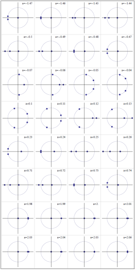
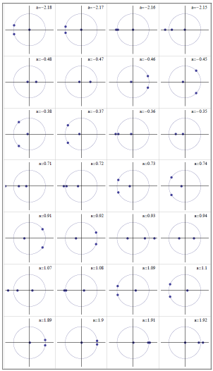
As we change the operating conditions of the trap, the parameters describing the system (23), i.e., the entries of the matrices and change. This results in a change in the solutions, and hence, the eigenvalues of the mapping at a period, . Suppose we start with a set of distinct eigenvalues on the unit circle, corresponding to a stable operating condition of the trap. The above list of possibilities ensures that as we tweak the parameters (the voltages), the eigenvalues of can move off the unit circle only if they “collide” on the unit circle first, meaning that instabilities develop through collisions of eigenvalues of unit magnitude. We will verify this prediction below, for the case of the coupled Mathieu equations.666Note that not all such collisions of eigenvalues result in instabilities. A more detailed discussion of these issues is given in [5] and [6].
3.2 Application to the Mathieu system
We next apply the general results reviewed above to the coupled Mathieu system, (20)-(21). We proceed as follows. For given, specific values for and , we loop over pre-chosen ranges of and . For each pair of values of and , we solve the equations (20)-(21) numerically, for four different initial conditions; we set one of , , , to one, and all the others to zero. After obtaining the four solutions over one period of the oscillating RF field (i.e., in terms of the time parameter , over a time period of ), we obtain , the “mapping at a period”, by joining the four column vectors ,
| (33) |
We then obtain the eigenvalues of this square matrix, and determine the stability properties of the system by checking the magnitudes of the eigenvalues. According to the discussion above, if all eigenvalues are distinct and are of unit magnitude, then the system is stable, and if there is an eigenvalue of magnitude larger than one, the system is unstable. We go beyond distinguishing between instability and stability, and also note whether the system is partially stable, having one pair of eigenvalues on the unit circle, and one pair away from it. While partial instability means instability in real life (since exciting only the stable subspace of solutions is impossible due to noise), the distinction between partial instability and full instability will help us below in our discussion of the multi-scale perturbation analysis.
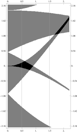
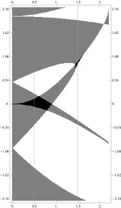
Looping over values of and and recording the stability properties of the system for each pair of values, we obtain a stability diagram for given values of and . We present two such plots below in Figures 2 and 5, the first one being an example of the classical, decoupled Mathieu system, and the second one being an example of the coupled case. As mentioned above, we go beyond the binary classification of stable vs. unstable points, and indicate regions of partial stability by using a shade of gray.
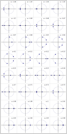
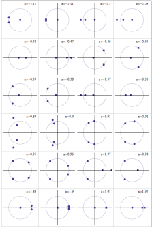
In Figures 3-4 and 6-7, we show how the eigenvalues evolve as one moves on the stability plot, moving across boundaries of stability. As predicted in our discussion above, changes in the degree of stability are accompanied by collisions of the eigenvalues on the unit circle. We will give a more comprehensive set of stability plots after we present an approximate analytical method (the method of multiple scales) for obtaining the stability boundaries.
4 The infinite determinant method
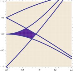
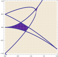
The “infinite determinant” approach to the stability analysis of the Mathieu equation [13] consists of substituting a modified Fourier expansion (a Floquet expansion) into the equations of motion and obtaining an infinite set of linear equations for the Fourier coefficients. These equations have nontrivial solutions only when the determinant of a certain infinite rank matrix (involving the parameters , , , ) vanishes. In practice, the infinite determinant is replaced by the determinant of a large-rank, finite matrix, and setting this determinant to zero gives approximate results. We will describe this method in the setting of the single variable Mathieu equation, explain how it can be generalized to the multi-variable case, and present plots for certain “simple” stability boundaries of the coupled system that can be obtained from this method in a straightforward way. These boundaries are in agreement with the results of the numerical approach described in the previous section.
Using Floquet’s theorem, we look for a solution to,
| (34) |
of the form,
| (35) |
Here, the infinite sum represents a periodic function with period equal to the period of the sinusoidal term in (34), and the exponential term in front determines the long time stability of the solution. The system is stable when is purely real, and unstable when has a nonvanishing imaginary part.777Positive imaginary parts result in decaying solutions, however, our discussion in Section 3 implies that such solutions are accompanied with solutions which have values with negative imaginary parts, i.e., those that grow unboundedly in time. Substituting (35) into (34) and shifting the summation index in two of the terms, we get,
| (36) |
Setting the coefficient of each basis functions to zero, we obtain an infinite set of equations for the coefficients . This set of equations has a solution only if the determinant of the infinite matrix of coefficients vanishes, i.e., , where,
| (37) |
The determinant of the matrix (37) does not converge as it stands,888We could remedy this by obtaining an alternative set of equations equivalent to (36) by dividing each equation derived from (36) by the corresponding diagonal entry, . Working with the matrix resulting from such an alternative set of equations results in a convergent determinant. however, in order to extract numerical results, we will work with a finite-size version of the matrix, and the convergence issue will not be of practical concern for the sizes and the numerical precision we will be working with.
Setting the determinant of to zero gives an equation that relates , , and the exponent . Once again, for given and , we can extract the growth factor, this time by solving the resulting algebraic equation. Checking whether the equation for has an imaginary solution allows us to deduce the stability/instability of the system for the given values of and . Looping over values of and and repeating the analysis would give the relevant stability plots. For the single variable case (or for the decoupled, two-variable case), it is possible to extract the stability boundaries directly, without looping over and and finding the transitions from stability to instability—it turns out [7] that for this case, setting the growth factor to gives equations that relate and on the stability boundaries.
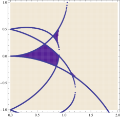
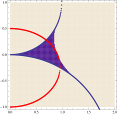
The generalization of the infinite determinant approach to the multi-variable case is straightforward, and involves replacing various scalars by vectors/matrices. One still gets a determinant equation relating , and , but in this case, not all stability boundaries can be obtained directly, without looping over and . Setting to as in the single variable case gives the stability boundaries that are related to the so-called “natural resonances”, but there is another set of stability boundaries, namely, those related to “combined resonances”, which cannot be obtained by this method. In [7], a pragmatic but unrigorous approach is proposed for obtaining the boundaries corresponding to the combined resonances, but we do not follow this procedure here. Instead, we only obtain the boundaries that are related to natural resonances, and compare the results with those we get from the numerical approach described in the previous section.
In Figures 8-11, we give the regions of complete stability obtained by the methods of the previous section, and the stability boundaries due to the “natural resonances”, obtained by the infinite determinant method described here. We choose , and show plots for 4 different values of . As can be seen, the boundaries obtained by the infinite determinant method bound the primary stability region accurately, except for the special case of .999We will give a more comprehensive set of stability plots in the following sections, where the behavior around will become more transparent. Smaller secondary stability regions, which move as the angle changes, also have two boundaries that are given accurately by the infinite determinant analysis. However, these regions also have a third boundary that is invisible to the method employed here, which is capable of getting only the boundaries due to natural resonances.
5 Method of multiple scales
For a given set of parameters, the Floquet analysis of Section 3.2 gives the stability regions of the coupled equations of motion numerically. While such results are useful, for asymmetric trap design and characterization, it would be beneficial to have at least approximate analytical formulae for the stability boundaries. Such approximate formulae would enable trap designers to quickly check the stability regions for a particular trap geometry, and would guide the trap design. Analogous results for the case of symmetric traps are well-known and useful.
One possible approach to this problem is to use straightforward perturbation theory of ordinary differential equations, which involves treating a certain parameter (, in our case) as small, and expanding the unknown solution into a power series in terms of this parameter. This gives separate equations for each power of the perturbation parameter, which are then solved order by order. While useful in many settings, this approach fails for a variety of problems due to the appearance of so-called “secular”, or “resonant” terms, which grow in time in an unbounded manner even when the exact solution is known to be bounded. This behavior invalidates the assumptions in the perturbation analysis after a certain time period. A straightforward perturbation expansion of the Mathieu equation results in such behavior.
Multi-scale perturbation theory, or the method of multiple scales, is a more sophisticated technique capable of avoiding such secular terms by expanding not only the solution, but also the independent parameter (typically, time) to a series in the small parameter. This results in a set of partial differential equations (PDEs) that collectively represent the ordinary diffential equation under consideration. The solutions of these PDEs are then restricted by imposing the condition that secular terms do not appear. The absence of secular terms allows the method of multiple scales to give uniformly accurate results for cases where standard perturbation theory gives results valid only for short time intervals. In this Section, we will use this technique to obtain approximate stability boundaries for the coupled system, (20)-(21). Since the calculations are a bit tedious, for readers only interested in the final results, we note that the approximate formulas for the stability boundaries are given in Equations (104), (105), (132) and (137).
The method of multiple scales has been applied to a wide variety of problems in physics, engineering, and applied mathematics. There are various conventions followed in the literature; below, we will use the approach described in [9] and [8]. For an elementary introduction to the method of multiple scales, see [14, 9]. For applications to the coupled Mathieu system, see [8, 15]. Note that the analyses in [8] and [15] are not immediately applicable to our case, since, as opposed to the cases covered in these references, some of the natural frequencies for the Paul traps we are considering are imaginary (i.e., one of the transverse directions is anti-confining).
5.1 Single-variable Mathieu equation
Let us first demonstrate the use of multi-scale perturbation theory on the relatively simple case of the single-variable Mathieu equation. After this example, we will work out the multi-scale perturbation analysis of the coupled system (20)-(21) describing asymmetric surface traps.
Preliminary discussion.
We would like to obtain approximate formulas for on the stability boundaries of the Mathieu equation,
| (38) |
This equation has multiple regions of stability separated by regions of instability; we will focus on the primary stability region near the origin of the - plane. We will treat as a small variable, and perform an expansion in its powers.
We begin the multi-scale perturbation analysis by introducing a set of slowly-varying time variables (the “multiple scales”),
| (39) |
We replace the dependent variable with a function of the s,
| (40) |
and expand it into a series in ,
| (41) |
The chain rule gives the derivative with respect to in terms of partial derivatives with respect to the time variables ,
| (42) |
Substituting (40), (41) and (42) into (38), one gets the equations for multi-scale perturbation theory. These equations give approximate solutions to (38) that are valid for small values of , unless is close to certain critical values. These critical values are of special interest to us, since they are the locations where the stability boundaries intersect the axis. Various approaches exist for dealing with these critical points; we will follow the technique used in [9], where one expands into a series, as well, around a critical point ,
| (43) |
In this approach, one obtains the stability boundaries by first getting conditions on , that ensure that the approximate solutions are bounded. These conditions give the critical values of these coefficients, and substituting these critical values back into (43), one gets the stability boundaries. It is noted in [8] that in order to get results accurate to order , it suffices to work with and . Accordingly, we will ignore and higher order “scales” and let .
The equations.
Using the notation , we have, up to second order in ,
| (44) | |||||
| (45) |
Substituting (44), (45) and (43) (where is arbirary, for now) in (38), we get,
Collecting terms with similar powers of and setting them to zero, we get the following partial differential equations:
| (46) | |||||
| (47) | |||||
| (48) |
As mentioned above, if the value of under consideration is away from a set of critical values, one can ignore and , set , and solve the equations (46)-(48) to obtain an approximate solution to (38). This approach, in fact, is how the critical points are obtained in the first place: we set , and obtain the special values of for which the approach fails (due to the appearence of “small denominators”). See, e.g., [9, 8] for a discussion and examples.
Here, we will skip this step, and just borrow the result that and are the two critical values relevant for the first stability region near the origin. We next perform expansions around these two points.
5.1.1 Expansion around
| (49) | ||||
| (50) | ||||
| (51) |
The general solution to (49) is,
| (52) |
where and are arbitrary functions. In order to suppress the secular term, i.e., the term that grows in time, we set . This gives,
| (53) |
Substituting (53) into (50), we get,
| (54) |
The solution for has a secular term proportional to ; in order to suppress unbounded growth, we set . Solving (54) with this assumption and setting to zero another secular term that appears (this term is analogous to the term in (52)), we get,
| (55) |
Substituting (53) and (55) in (51) and using , we get,
In order to avoid terms in that grow linearly in , we must have,
This equation will have non-growing solutions for if and only if,
Combining the conditions , , and , we see that the curve in the - plane separating bounded solutions from unbounded ones around , is given by,
| (56) |
with being the stable region.
5.1.2 Expansion around
| (57) | |||||
| (58) | |||||
| (59) |
The general solution of (57) is,
| (60) |
Plugging this in (58), we get,
| (61) |
The solutions of this equation will have growing parts unless the coefficients of the “resonance terms” and on the right hand side vanish. This gives,
| (62) | |||||
| (63) |
This system will have exponentially growing solutions if , and oscillatory solutions if . Thus, the critical values of are . Assuming , the general solution is,
| (64) | |||||
| (65) |
where and and are constants. After substituting (64)-(65) in (61) and setting the resulting resonant terms to zero, we get,
| (66) |
whose general solution is,
| (67) |
Plugging (67) in (59), the right hand side of (59) ends up having various terms proportional to and . Once again, these resonant terms will result in growing solutions for , so we set their coefficients to zero. This gives,
| (68) | |||||
| (69) |
Recalling and from above (see (64-65)), we get,
| (70) | |||||
| (71) |
Combining these equations, using the explicit solution (64-65) for and and once again requiring the absence of resonant terms, we get,
| (72) |
Finally, combining the conditions for , and , we get the formula for the stability boundaries near , as,
| (73) | |||||
| (74) |
with the region between the two curves corresponding to unstable solutions, and the region outside corresponding to stable ones. The results (56) and (74) are in agreement with the classical results for Mathieu equation.
5.2 Two-variable, coupled Mathieu’s equations
We next turn to the coupled Mathieu system (20)-(21), which we reproduce here:
| (77) | |||||
| (78) |
These equations describe the radial motion of an ion in an asymmetric trap with decoupled axial motion. Recall that the coordinates are chosen to be along the DC principal axes, and the constants and are given in terms of the relative angle between the RF and DC axes as,
| (79) | |||||
| (80) |
As in the single variable case, we begin the multi-scale analysis by promoting and to functions of two separate time variables, and , and expanding them to series in ,
| (81) | |||||
| (82) |
If is near a critical value where this expansion fails to work, we expand as well,
| (83) |
Working to second order in , and collecting terms with similar powers of , we get,
| (84) | ||||
| (85) | ||||
| (86) | ||||
for (77), and,
| (87) | ||||
| (88) | ||||
| (89) | ||||
for (78). Following our discussion in Section 3.2, we will assume . For , the critical values are and (once again we will skip the justification for these values, and refer the reader to [8]). The expansion around will proceed similarly to the single variable case, but the case requires special attention. Assuming and , we see that the solutions of (84) are oscillatory, but the ones for (87) are exponential.
Assuming that the initial conditions of the system are fine-tuned so that the unbounded solutions are not excited, one can investigate the bounded part of the general solution. However, as mentioned in our discussion in Section 3.2, noise will undoubtedly excite the unstable solutions in practice.
Nevertheless, our stability plots obtained by the techniques of Section 3.2 suggest that the curves separating regions of partial stability from those of full instability may in fact be of some use. We observe from the stability plots of Figures 2 and 5 (and from additional plots we will present below) that the primary stability region around the origin is bounded by an extension of such curves. In other words, the curves emanating at the critical point begin as boundaries between regions of full instability and regions of partial instability, but once they intersect with the stability boundaries emanating from , they become boundaries between full instability and full stability. Motivated by this empirical observation, we will obtain formulas for the curves emanating at the critical point , and use them as stability boundaries after they intersect with the curves emanating from . We will demonstrate the reliability of this approach in the stability plots we present below.
5.2.1 Expansion around
We begin with the expansion around . Setting in equations (84)-(89), we get,
| (90) | ||||
| (91) | ||||
| (92) | ||||
and,
| (93) | ||||
| (94) | ||||
| (95) | ||||
Solving (90) and (93) and setting the secular terms to zero, we get,
| (96) | |||||
| (97) |
Substituting these in (91) and (94) gives,
| (98) | |||||
| (99) |
In order to avoid growing and , we need to pick . Solving (98) and (99) with this assumption and setting the coefficients of two other secular terms that grow linearly in to zero, we get,
| (100) | |||||
| (101) |
Plugging the solutions (96), (97), (100), (101) in (92) and (95), we get equations for and . These will have bounded solutions only if the -independent terms on the right hand sides of the equations add up to zero. Asserting this condition gives,
| (102) | |||||
| (103) |
Equations (102) and (103) will have oscillatory solutions for and when , and when , respectively. Using (79) and (80), we have, . Assuming , we see that simulatenous stability occurs for . In other words, the stability boundaries around are given by,
| (104) | |||||
| (105) |
Note that these conditions are what would be obtained from separate stability analyses of (77) and (78), respectively, if the coupling terms in those equations were ignored and the single-variable results (56) and (76) of Section 5.1.1 were used.
5.2.2 Expansion around
We next expand around . As mentioned above, in this case we will seek solutions with partial stability. For , (84)-(86) become,
| (106) | |||||
| (107) | |||||
| (109) | |||||
| (110) | ||||
| (111) | ||||
| (112) | ||||
The general solution to (106) is,
| (113) |
Assuming , the solution to (110) is exponential,
| (114) |
This shows that the general solution to the coupled system is unstable for , , as discussed above. In order to investigate partial stability, we set the coefficients of the exponential solutions to zero, , which gives . Substituting this and (113) in (107), and setting the coefficients of and on the right hand side to zero in order to avoid resonant (secular) terms that would result in growing solutions for , we get,
| (115) | |||||
| (116) |
Combining these, we get,
| (117) | |||||
| (118) |
which will have oscillatory solutions if and exponential ones if . Thus, the critical values for partial stability are,
| (119) |
The oscillating solutions for and are given as,
| (120) | |||||
| (121) |
where , and and are constants.
After having ensured that the resonant terms in (107) vanish by enforcing (115) and (116), we can solve (107) to get the oscillatory solutions for . We get,
| (122) |
Similarly, substituting the solution (113) in (111), we get a bounded solution for after setting the coefficients of the exponential terms to zero:
| (123) |
We next substitute (122) and (123) into (109) and collect the resonance terms, i.e., terms proportional to and , on the right hand side. Setting the coefficients of these resonances to zero in order to avoid growing solutions for , we get,
| (129) | |||||
| (130) |
Now, since the solutions (120) and (121) for and are in resonance with the left hand sides of (129) and (130), in order to avoid growing solutions,
the coefficients on the right hand sides of these equations must vanish. Using (119), this gives,
| (131) |
Thus, the second order approximation to the relevant stability boundary starting at is given as,
| (132) |
where we picked the negative sign for the first order term in order to get the curve that approximates the upper boundary of the primary stability region.
Boundary of the primary stability region.
In order to obtain the approximate boundaries of the primary stability region, we also need to find an approximate formula for the stability boundary that emanates from negative when . Our expansion around was based on the assumption that , so that had oscillatory solutions to zeroth order, and had exponential ones. In order to obtain the curves for negative , we just replace the roles of and by a series of redefinitions. Namely, we set,
| (133) |
These redefinitions transform the equations of motion (77) and (78) into exactly the same form, with the variables (except and ) being replaced by their tilded counterparts,
| (134) | |||||
| (135) |
Now, if , the transformation (133) makes , thus, we can apply (132) to (134)-(135) by replacing all the quantities in (132) by their tilded counterparts. This gives,
| (136) |
or, equivalently,
| (137) |
This gives the required approximate boundary of the primary stability region for . Note that the curve starts at .
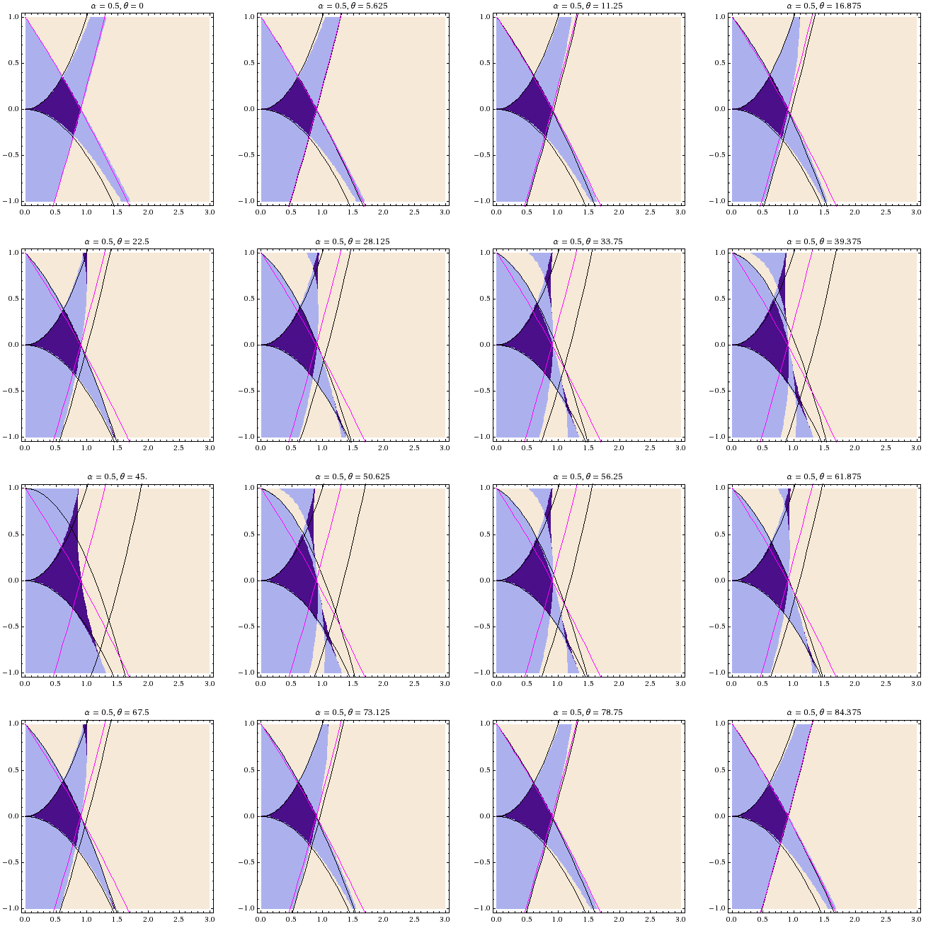
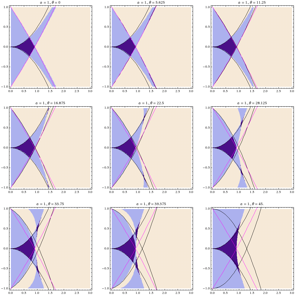
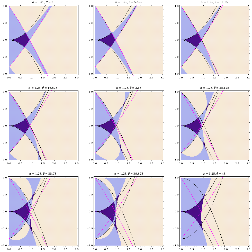
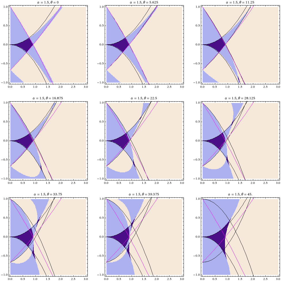
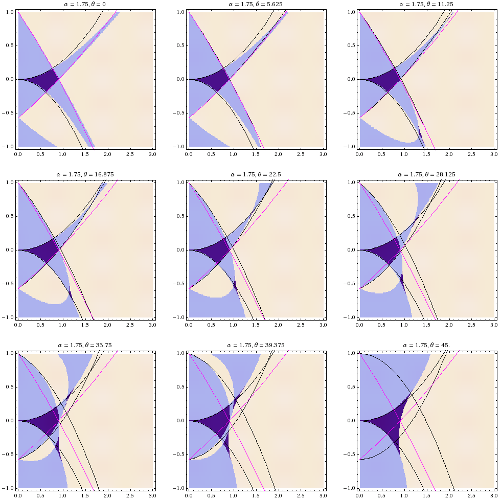
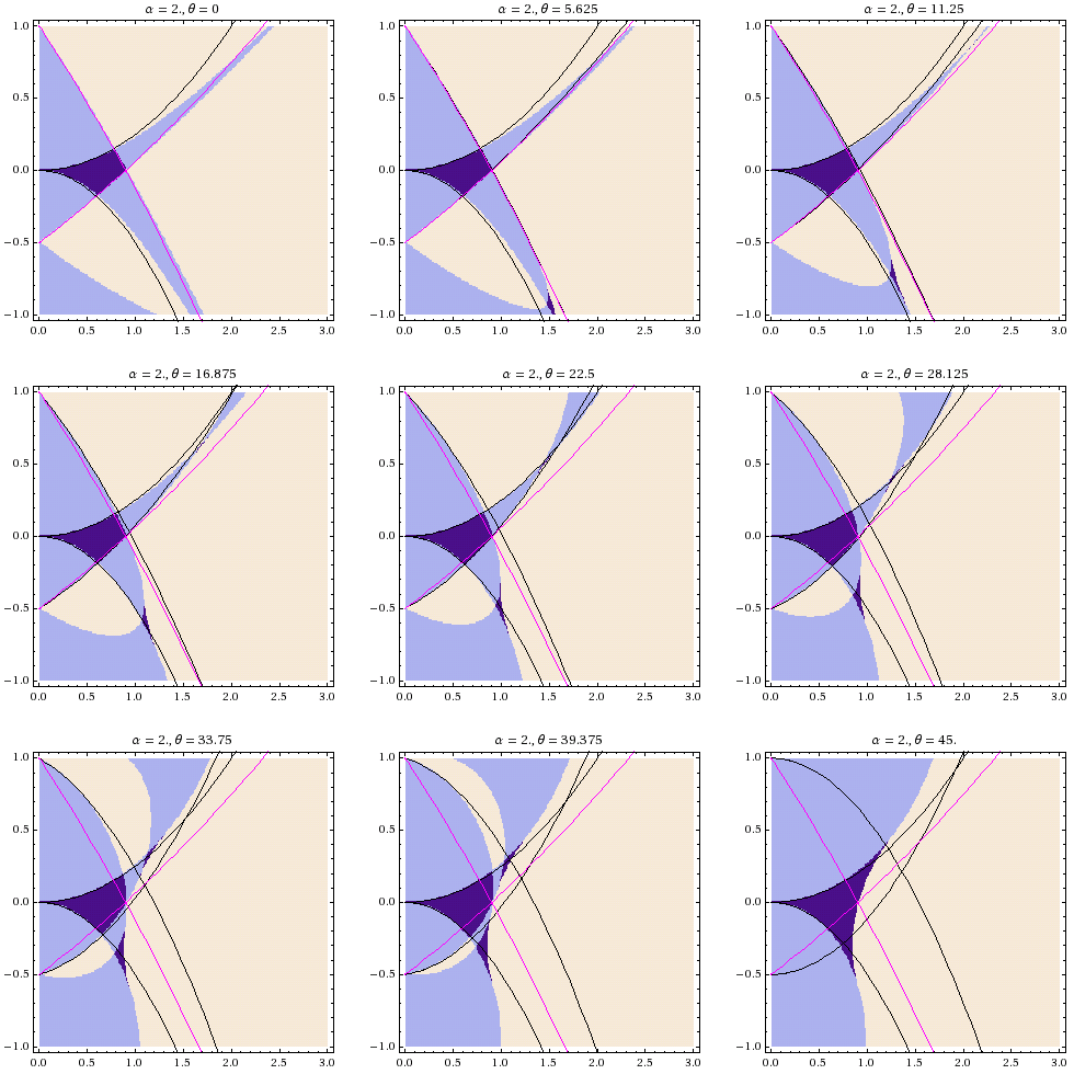
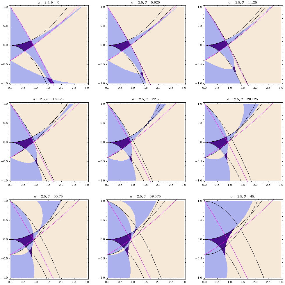
In Figures 12-18, we compare the results of this section with the results from the numerical analysis of Section 3.2, for various values of and .101010In Figure 12, we do not show the plot for since it is the same as the plot for . In fact, as can be seen from the figure, the stability behavior of the system is symmetric around , in the sense that the plots for and are identical. This is due to the fact that the equations of motion are invariant under the transformation , . Since the system is symmetric under reflections of the axis, this transformation should leave the stability plot invariant. In Figures 13-18, we only show the stability plots for between and .
6 Conclusions and discussion
In Figures 12-18, we present the results of our stability analysis. We compare the results of the numerical method of Section 3.2 (purple areas) to the stability boundaries obtained by the multi scale perturbation analysis (black lines). We show plots for a range of angles between the RF and DC axes, and a range of s (recall equations (20)-(21)). A few important conclusions are evident from the plots.
-
•
The primary stability region does not get smaller when a nonzero angle is introduced between the RF and DC axes if the other variables are kept fixed. Such a nonzero angle between RF and DC fields represents the case of an asymetric surface electrode geometry and/or asymmetric voltages.
-
•
Although the primary stability region does not change appreciably when is varied, two secondary stability regions are highly variable, and when has the special value of , they join the primary region to result in an exceptionally large region of stability.
-
•
The curves obtained from multi-scale perturbation theory approximate the boundaries of partial stability111111If there is a set of initial conditions for which the ion motion is bounded and another set for which it is unbounded, we call the system partially stable. Since it is impossible to tune the system perfectly, the unbounded solutions of a partially stable operating point of the trap will get excited in practice, and the ions will be lost. quite accurately when is near zero. Regions of partial stability become regions of full stability when they “overlap” near the primary stability region of classical, symmetric traps. Unfortunately, in this region, is likely large enough to make the accuracy of the approximation unsatisfactory, especially for angles close to the critical value of . Since, in practice, partial stability means instability, the small region, where our multi-scale formulas are uniformly accurate, is not of relevance to the practical problem of the stability of ion motion.
-
•
When we lay the approximate stability boundaries for the symmetric Paul trap (described by decoupled equations) on top of the coupled stability plots, we see that these boundaries consistently underestimate the size of the stability region for the coupled system.
A relative angle between the RF and DC axes does not change the boundaries of the primary stability region significantly, unless the angle is close to , in which case the stability region is enhanced. However, the shapes and locations of a pair of secondary stability regions are highly dependent on the relative angle.
The conclusion of this analysis for the practical problem of asymmetric ion trap design and operation is as follows: Just as in the case of symmetric Paul traps, the - stability plot of the standard single-variable Mathieu equation is sufficient to allow one to determine stable operating conditions for asymmetric surface traps with long RF electrodes. It is possible to proceed as in the case of symmetric Paul traps, by obtaining a pair of “” values for the two radial principal axes of the DC potential, and a pair of “” values for the two radial principal axes of the RF potential. Ignoring the fact that there is a nonzero relative angle between the RF and DC axes, the two decoupled Mathieu equations for these pairs can be used to determine the stability properties of the coupled system. This approach does not give precise stability boundaries for asymmetric traps, but it is “safe” in the sense that trap operating conditions deemed stable by this method will in fact be stable for the coupled system. By ignoring the coupling, the size of the primary stability region is simply underestimated.
Acknowledgements.
We would like to thank Alexa W. Harter, Jason M. Amini, Curtis Volin, and Richart E. Slusher for helpful comments and discussions. This material is based upon work supported by the Office of the Director of National Intelligence (ODNI), Intelligence Advanced Research Projects Activity (IARPA) and the Defense Advanced Research Projects Agency (DARPA). All statements of fact, opinion or conclusions contained herein are those of the authors and should not be construed as representing the official views or policies of IARPA, the ODNI, or the U.S. Government. US Army Research Office contract support through W911NF081-0315, W911NF081-0515, and W911NF071-0576 is acknowledged.
References
- [1] J. Chiaverini, RB Blakestad, J. Britton, JD Jost, C. Langer, D. Leibfried, R. Ozeri, and DJ Wineland. Surface-electrode architecture for ion-trap quantum information processing. Arxiv preprint quant-ph/0501147, 2005.
- [2] J. Kim and C. Kim. Integrated optical approach to trapped ion quantum computation. Arxiv preprint arXiv:0711.3866, 2007.
- [3] G.R. Brady, A.R. Ellis, D.L. Moehring, D. Stick, C. Highstrete, K.M. Fortier, M.G. Blain, R.A. Haltli, A.A. Cruz-Cabrera, R.D. Briggs, et al. Integration of fluorescence collection optics with a microfabricated surface electrode ion trap. Applied Physics B: Lasers and Optics, pages 1–8, 2010.
- [4] D.J. Wineland, C. Monroe, WM Itano, D. Leibfried, BE King, and DM Meekhof. Experimental issues in coherent quantum-state manipulation of trapped atomic ions. Arxiv preprint quant-ph/9710025, 1997.
- [5] V.I. Arnold. Mathematical methods of classical mechanics. Springer, 1989.
- [6] AP Seyranian, ON Kirillov, and AA Mailybaev. Coupling of eigenvalues of complex matrices at diabolic and exceptional points. Journal of Physics A: Mathematical and General, 38:1723, 2005.
- [7] J. Hansen. Stability diagrams for coupled Mathieu-equations. Archive of Applied Mechanics, 55(6):463–473, 1985.
- [8] A.H. Nayfeh, D.T. Mook, and Ebooks Corporation. Nonlinear oscillations, volume 31. Wiley Online Library, 1979.
- [9] A.H. Nayfeh and Ebooks Corporation. Perturbation methods, volume 6. Wiley Online Library, 1973.
- [10] MG House. Analytic model for electrostatic fields in surface-electrode ion traps. Physical Review A, 78(3):033402, 2008.
- [11] F.G. Major, V.N. Gheorghe, and Gunther. Werth. Charged particle traps. Springer-Verlag Berlin Heidelberg, 2005.
- [12] P.K. Ghosh. Ion traps. Clarendon Press New York: Oxford University Press, Oxford, 1995.
- [13] ET Whittaker and GN Watson. A course of modern analysis. Cambridge Mathematical Library. Cambridge University Press, Cambridge, 1996.
- [14] J. Kevorkian and J.D. Cole. Multiple scale and singular perturbation methods. Springer Verlag, 1996.
- [15] G.M. Mahmoud. Stability regions for coupled Hill’s equations. Physica A: Statistical and Theoretical Physics, 242(1-2):239–249, 1997.