Deconstructing Approximate Offsets.

Abstract

We consider the offset-deconstruction problem: Given a polygonal shape $Q$ with $n$ vertices, can it be expressed, up to a tolerance $\varepsilon$ in Hausdorff distance, as the Minkowski sum of another polygonal shape $P$ with a disk of fixed radius? If it does, we also seek a preferably simple-looking solution $P$; then, $P$’s offset constitutes an accurate, vertex-reduced, and smoothened approximation of $Q$. We give an $O(n\log n)$-time exact decision algorithm that handles any polygonal shape, assuming the real-RAM model of computation. A variant of the algorithm, which we have implemented using the cgal library, is based on rational arithmetic and answers the same deconstruction problem up to an uncertainty parameter $\delta$; its running time additionally depends on $\delta$. If the input shape is found to be approximable, this algorithm also computes an approximate solution for the problem. It also allows us to solve parameter-optimization problems induced by the offset-deconstruction problem. For convex shapes, the complexity of the exact decision algorithm drops to $O(n)$, which is also the time required to compute a solution $P$ with at most one more vertex than a vertex-minimal one.

1 Introduction

The $r$-offset of a polygon, for a real parameter $r>0$, is the set of points at distance at most $r$ away from the polygon. Computing the offset of a polygon is a fundamental operation. The offset operation is, for instance, used to define a tolerance zone around the given polygon [11] or to dilute details for clarity of graphic exposition [16, 20, 4]. Technically, it is usually computed as the Minkowski sumof the polygon and a disk of radius $r$. The resulting shape is bounded by straight-line segments and circular arcs. However, a customary practice is to model the disk in the Minkowski sum with a (tight) polygon, which yields a piecewise-linear approximation of the offset. Our study is motivated by two applications, where such an approximation forms the legacy data which a program has to deal with—the original shape before offsetting is unknown. This leads us to the question what is the original polygon whose approximate offset we have at hand. Of course, finding the exact original polygon, or even its topology, is impossible in general, because the offset might have blurred small features like holes or dents. However, a reasonable choice can lead to a more compact and smooth representation of the approximate offset.

The first relevant problem concerns cutting polygonal parts out of wood. A wood-cutting machine, which can smoothly cut along straight line segments and circular arcs, is given a plan to cut out a certain shape. This shape was designed as a polygon expanded by a small offset, but with circular arcs approximated by polygonal lines comprising many tiny line segments. Thus instead of moving smoothly along circular arcs, the cutting tool has to move along a sequence of very short segments, and make a small turn between every pair of segments. The process becomes very slow, the tool heats up, and occasionally it causes the wood to burn. Moving the cutting tool smoothly and fast enough is the way to keep it cool. If this were the only issue, other smoothing techniques like arc-spline approximation [5, 12] may have been applicable. However, we may also wish to reduce the offset radius if a more accurate cutting machine is available—in this case, it seems desirable to find the original shape first and then to re-offset with a smaller radius.

A motivation to study this question from a different domain is to recover shapes sketched by a user of a digital pen and tablet. The pen has a relatively wide tip, and the input obtained is in fact an approximate offset (with the radius of the pen tip) of the intended shape. The goal is to give a good polygonal approximation of the intended shape. More broadly, as the offset operation is so commonplace, it seems natural to ask, given only an (approximated) offset shape, what could be the original shape before the offsetting. Therefore, we pose the (offset-)deconstruction problem which comes in two variants:

• Given a polygonal shape $Q$, and two real parameters $r,\varepsilon>0$, decide if there exists a polygonal shape $P$ such that $Q$ is within (symmetric) Hausdorff-distance $\varepsilon$ to the $r$-offset (i.e., offset with radius $r$) of $P$

• If the answer to Problem 1 is YES, compute a polygonal shape $P$ with the desired property. We refer to $P$ as a solution of the deconstruction problem. Note that $P$ might be disconnected, even if $Q$ is connected (Figure 1.1).

Problem 1 can be seen as a special case of the Minkowski decomposition problem which asks whether a set can be composed in a non-trivial way as the Minkowski sum of two sets—disallowing a summand to be a homothetic copy of the input set. A general criterion for decomposability of convex sets in arbitrary dimension has been presented in [19]. A particularly well-studied case are planar lattice polygons, because of their close relation to problems in algebra, for instance, polynomial factorization [17]. It has been shown that deciding decomposability is NP-complete for lattice polygons [8]. In [6], decomposability is investigated under the constraint that one of the summands is a line segment, a triangle, or a quadrangle. However, all these approaches discuss the exact decomposition problem; our scenario of being Hausdorff-close to a particular decomposition seems to not have been addressed in the literature. Allowing tolerance raises interesting algorithmic questions and at the same time makes the tools that we develop more readily suitable for applications, which typically have to deal with inaccuracies in measuring and modeling.

Figure 1.1: For a given $Q$, the red $P$ is a candidate summand whose exact $r$-offset is shaded. Left: For a given $\varepsilon$, deconstruction is ensured iff $\phi_{1}\leq\varepsilon$ and $\phi_{2}\leq\varepsilon$. Note that, when $r$ decreases, $\phi_{1}$ decreases, but $\phi_{2}$ increases. Middle: Example where $Q$ can be approximated by an $r$-offset of a $P$ that has much fewer vertices than $Q$. Right: Example where $Q$ can be approximated by the $r$-offset of a disconnected shape $P$.

Contributions. We first present an efficient algorithm to decide Problem 1: For a shape $Q$ with $n$ vertices, the algorithm reports the correct answer in $O(n\log n)$ time in the real-RAM model of computation [18]. It constructs offsets with increasing radii in three stages; the intermediate shapes arising during the computation are in general more difficult to offset than polygons, as they are bounded by straight-line segments and “indented” circular arcs (namely, the shape is locally on the concave side of the arcs). The main observation is that for certain classes of such shapes, these circular arcs can be ignored when computing the next offset (see Theorem 5 for the precise statement). This observation bounds the time required by each offset computation by $O(n\log n)$, which is the key to the efficiency of the decision algorithm. Our proof is constructive, that is, if a solution exists it can be computed with the same running time.

The computation of the exact decision procedure requires the handling of algebraic coordinates of considerably high degree. As an alternative, we give an approximation scheme that works exclusively with rational numbers. The scheme proceeds by replacing the offset disks by polygonal shapes of similar diameter, whose precision is determined by another parameter $\delta<\varepsilon$. We prove a bound $\Delta$ that depends on ${\hat{\varepsilon}}$, the minimal $\varepsilon$ for which the answer to the decision problem is YES, such that the rational approximation returns the exact result for all $\delta\leq\Delta$. If the input shape is found to be deconstructible, this algorithm also outputs a solution. The computation of ${\hat{\varepsilon}}$ up to any desired precision is still possible. We believe that our investigation of the relation between $\delta$ and ${\hat{\varepsilon}}$ is of independent relevance, mostly to the study of certified algorithms that approximate geometric objects with algebraic coordinates by means of rational arithmetic.

The deconstruction problem leads to natural optimization questions: if $Q$ and $r$ are given, how to compute ${\hat{\varepsilon}}$, the minimal tolerance for which a solution exists? Similarly, if $Q$ and $\varepsilon$ are given, what are the possible radii such that a solution exists? For the first question, we provide a certified and efficient solution based on binary search, using the rational approximation algorithm. For the second question, we prove that the set of possible radii forms an interval and propose an algorithm to compute it. We also provide a heuristic to find a reasonable radius $r$ if both $r$ and $\varepsilon$ are unknown.

For a convex shape $Q$ with $n$ vertices, we reduce the running time for solving Problem 1 to the optimal $O(n)$ (in the real-RAM model). Moreover, we describe a greedy algorithm within the same time complexity that returns a solution $P^{\star}$ which minimizes, up to one extra vertex, the number of vertices among all solutions, if there are any. Our algorithm technically resembles an approach for the different problem of finding a vertex-minimal polygon in the annulus of two nested polygons [1]. We also remark that the $r$-offset of $P^{\star}$ has a tangent-continuous boundary and therefore constitutes a special case of an arc-spline approximation of $Q$ where all circular arcs have the same radius.

Organization. We describe an exact decision algorithm for the deconstruction problem (solving Problem 1 above) in Section 2. In Section 3 we describe a rational-approximation algorithm for the deconstruction problem. Both algorithms output a solution in case the input is deconstructible (solving Problem 2). Section 4 discusses the optimization problems. For convex input, Section 5 exposes a specialized deconstruction algorithm and the computation of an almost vertex-minimal solution. We conclude in Section 6 by pointing out open problems.

2 The Decision Algorithm

For a set $X\subset\mathbb{R}^{2}$ denote its boundary by $\partial X$ and its complement by $X^{C}:=\mathbb{R}^{2}\setminus X$. A polygonal region or polygonal shape $X\subset\mathbb{R}^{2}$ is a set whose boundary consists of finitely many line segments with disjoint interiors. The endpoints of these straight-line segments are the vertices of the polygonal region. We assume henceforth that the input shapes that we deal with are bounded (but not necessarily connected). Although the techniques seem to go through also for unbounded shapes, this assumption simplifies the exposition and is sufficient for the real-life applications we have in mind. For two sets $X$ and $Y$, we denote their Minkowski sum by $X\oplus Y:=\{x+y\mid x\in X,y\in Y\}$. With $d(\cdot,\cdot)$ the Euclidean distance function, and any $c\in\mathbb{R}^{2},r\in\mathbb{R}$, we write $D_{r}(c):=\{p\in\mathbb{R}^{2}\mid d(c,p)\leq r\}$ for the (closed) $r$-disk around $c$, and $D_{r}:=D_{r}(O)$ for the $r$-disk centered at the origin. The $r$-offset of a set $X$, $\mathrm{offset}(X,r)$, is the Minkowski sum  $X\oplus D_{r}$.

For $p\in\mathbb{R}^{2}$ and $X$ a closed set, we write $d(p,X):=\min\{d(p,x)\mid x\in X\}$. The (symmetric) Hausdorff distance of two closed point sets $X$ and $Y$ is $H(X,Y):=\max\{\max\{d(x,Y)\mid x\in X\},\max\{d(y,X)\mid y\in Y\}\}.$ We say that $X$ is $\varepsilon$-close to $Y$ (and $Y$ to $X$) if $H(X,Y)\leq\varepsilon$, which can also be expressed alternatively:

Proposition 1.

For $X,Y$ closed, $X$ is $\varepsilon$-close to $Y$ if and only if $Y\subseteq\mathrm{offset}(X,\varepsilon)$ and $X\subseteq\mathrm{offset}(Y,\varepsilon)$.

Decision algorithm. We fix $r>0$, $\varepsilon>0$, and a polygonal region $Q$, and consider the following question: Is there a polygonal region $P$ such that $Q$ and the $r$-offset of $P$ have Hausdorff-distance at most $\varepsilon$? First of all, we can assume that $r>\varepsilon$; otherwise, we can choose $P:=Q$, because $\mathrm{offset}(Q,r)$ and $Q$ have Hausdorff-distance at most $\varepsilon$. We define another operation, $r$-inset (a.k.a. “erosion”), which is computationally similar to an offset:

Definition 2.

For $r>0$, and $X\subset\mathbb{R}^{2}$, the $r$-inset of $X$ is the set $\mathrm{inset}(X,r):=\mathrm{offset}(X^{C},r)^{C}=\left\{x\in\mathbb{R}^{2}\mid D_{r}(x)\subseteq X\right\}.$

We are now ready to present the decision algorithm:

Algorithm 1 Decide($Q,r,\varepsilon$)

1. $Q_{\varepsilon}\leftarrow\mathrm{offset}(Q,\varepsilon)$

2. $\Pi\leftarrow\mathrm{inset}(Q_{\varepsilon},r)$

3. $Q^{\prime}\leftarrow\mathrm{offset}(\Pi,r+\varepsilon)$

4. if $Q\subseteq Q^{\prime}$ then return YES else return NO

We next prove that Decide (Algorithm 1) correctly decides whether $Q$ is $\varepsilon$-close to some $r$-offset of a polygonal region. A first observation is that for any polygonal region $P$, $\mathrm{offset}(P,r)\subseteq Q_{\varepsilon}$ if and only if $P\subseteq\Pi$. This is an immediate consequence of the definition of the inset operation. This shows that for any $\mathrm{offset}(P,r)$ that is $\varepsilon$-close to $Q$, $P$ must be inside $\Pi$. Moreover, it shows that any choice of $P\subseteq\Pi$ already satisfies one of Proposition 1’s inclusions. It is only left to check whether $Q\subseteq\mathrm{offset}(\mathrm{offset}(P,r),\varepsilon)=\mathrm{offset}(P,r+\varepsilon)$. We summarize:

Proposition 3.

$Q$ is $\varepsilon$-close to $\mathrm{offset}(P,r)$ if and only if $P\subseteq\Pi$ and $Q\subseteq\mathrm{offset}(P,r+\varepsilon)$.

To prove correctness of Decide, we have to show that $Q\subseteq\mathrm{offset}(\Pi,r+\varepsilon)$ already implies that there also exists a polygonal region $P\subseteq\Pi$ with $Q\subseteq\mathrm{offset}(P,r+\varepsilon)$. The main difficulty in proving this is that $\Pi$ is not polygonal in general; we have to study its shape closer to prove that we can approximate it by a polygonal region, maintaining the property that the offset remains $\varepsilon$-close to $Q$.

The shape of offsets and insets. For a polygonal region $Q$, it is not hard to figure out the shape of $Q_{\varepsilon}=\mathrm{offset}(Q,\varepsilon)$: It is a closed set bounded by straight-line segments and by circular arcs, belonging to a circle of radius $\varepsilon$. It is important to remark that all circular arcs are bulges:

Definition 4.

Let $X\subset\mathbb{R}^{2}$ be a closed set with some circular arc $\gamma$ on its boundary. Then, $\gamma$ is called a dent with respect to $X$, if each line segment connecting two distinct points on $\gamma$ is not fully contained in $X$. Otherwise, the arc is called a bulge.

We call $X$ a bulged (resp. an indented) region with radius $r$, if $\partial X$ consists of finitely many straight-line segments and bulges (resp. dents) that are all of radius $r$, interlinked at the vertices of the region.

Note that a bulged region (left) is not necessarily convex. The $r$-offset of a polygonal region $P$ is a bulged region with radius $r$. The heart of this section is Theorem 5 showing that the same also holds if $P$ is an indented region (right) with radius smaller than $r$:

Theorem 5.

Let $P$ be an indented region with radius $r_{1}$, and let $r_{2}>r_{1}$. Then, there is a polygonal region $P_{L}\subseteq P$ such that $\mathrm{offset}(P,r_{2})=\mathrm{offset}(P_{L},r_{2})$. In particular, $\mathrm{offset}(P,r_{2})$ is a bulged region with radius $r_{2}$.

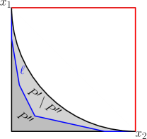
(a)

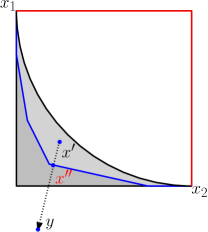
(b)

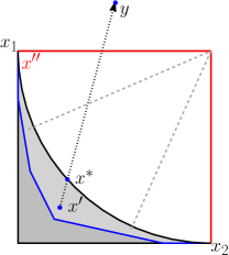
(c)

Figure 2.1: (a) The (extended) linear cap split by the polyline $\ell$, (b-c) the two cases in the proof of Theorem 5.

Proof.

After possibly splitting circular arcs into at most four parts, we can assume that each circular arc spans at most a quarter of the circle. For such a circular arc, we define its endpoints by $x_{1}$ and $x_{2}$, and denote the linear cap of the circular arc as the (closed) indented region enclosed by the circular arc, and the two lines tangent to the circle through $x_{1}$ and $x_{2}$ (the shaded area in Figure 2.1a). The extended linear cap is the (polygonal) region spanned by the two tangents just mentioned, and the two corresponding normals at $x_{1}$ and $x_{2}$. Clearly, the normals meet in the center of the circle that defines the arc.

We iteratively replace a indented arc of an indented region $P^{\prime}$ with radius $r_{1}$ (initially set to $P$) by a polyline $\ell$ ending in the endpoints of the circular arc, such that $\ell$ does neither leave $P^{\prime}$ nor the linear cap of the circular arc, and such that other boundary parts of $P^{\prime}$ are not intersected. This yields another indented region $P^{\prime\prime}$ with radius $r_{1}$, where one indented arc is replaced by a polyline, as depicted in Figure 2.1a. Iterating this construction, starting with $P$, until all indented arcs are replaced, we obtain a polygonal region $P_{L}$.

We show that in each iteration, the $r_{2}$-offsets of $P^{\prime}$ and $P^{\prime\prime}$ are the same. For that we consider any point $x^{\prime}\in P^{\prime}\setminus P^{\prime\prime}$, in the region that is cut off by $P^{\prime\prime}$, and consider $y=x^{\prime}+v^{\prime}$ for an arbitrary $v^{\prime}\in D_{r_{2}}$. We show that in all cases, $y$ can also be written by $y=x^{\prime\prime}+v^{\prime\prime}$, with $x^{\prime\prime}\in P^{\prime\prime}$, and $v^{\prime\prime}\in D_{r_{2}}$.

Since the circular arc spans at most a quarter of the circle, it is easily seen that $D_{r_{1}}(x_{1})\cup D_{r_{1}}(x_{2})$ covers the whole extended linear cap. Therefore, for any $y$ that lies within the extended linear cap, selecting $x^{\prime\prime}=x_{1}$ or $x^{\prime\prime}=x_{2}$, we get $y=x^{\prime\prime}+v^{\prime\prime}$ with $v^{\prime\prime}\in D_{r_{1}}$.

We distinguish two other cases: for $y$ that lies outside of the extended linear cap $v^{\prime}=\overline{x^{\prime}y}$ crosses either $\ell$ or the circular arc. In the former case, we can simply pick the crossing point as $x^{\prime\prime}$, and set $v^{\prime\prime}\in D_{r_{2}}$ accordingly (Figure 2.1b). In the latter case, let us denote the crossing point as $x^{*}$ (Figure 2.1c). We consider the set of points that is closer to $x^{*}$ than to $x_{1}$ and $x_{2}$. Clearly, that region is bounded by the two corresponding bisectors, which meet in the center of the circle that defines the circular arc and is therefore completely contained within the extended linear cap. It follows that $y$ is closer to one of the endpoints of the arc, say $x_{1}$, than to $x^{*}$. Selecting $x^{\prime\prime}=x_{1}$ we ensure $y$ is closer to $x^{\prime\prime}$ than to $x^{\prime}$, which proves that $y=x^{\prime\prime}+v^{\prime\prime}$ with some $v^{\prime\prime}\in D_{r_{2}}$ in this case as well. ∎

The proof of Theorem 5 implies that $\mathrm{offset}(P,r_{2})$ for such a region $P$ is completely determined by the offset of its linear segments, and the offset of the endpoints of circular arcs: the interior of the indented circular arcs can be ignored.

Corollary 6.

Algorithm 1 (Decide) returns YES if and only if there exists a polygonal region $P$ such that $\mathrm{offset}(P,r)$ is $\varepsilon$-close to $Q$.

Proof.

$Q_{\varepsilon}$ is a bulged region with radius $\varepsilon$. Therefore, $Q_{\varepsilon}^{C}$ is an indented region with the same radius. Since $r>\varepsilon$, Theorem 5 implies that $\mathrm{offset}(Q_{\varepsilon}^{C},r)$ is a bulged region with radius $r$, and so, $\mathrm{offset}(Q_{\varepsilon}^{C},r)^{C}=\mathrm{inset}(Q_{\varepsilon},r)=\Pi$ is an indented region with the same radius. Using $r+\varepsilon>r$ and applying Theorem 5 once more, there exists a polygonal region $P\subseteq\Pi$ such that $\mathrm{offset}(\Pi,r+\varepsilon)=\mathrm{offset}(P,r+\varepsilon)$. It follows that, if the algorithm returns YES, there is indeed a polygonal region $P$ whose $r$-offset is $\varepsilon$-close to $Q$. If the algorithm returns NO, it is clear that no such polygonal region can exist. ∎

Theorem 7.

Let $P$ be an indented region with radius $r_{1}$ having $n$ vertices, and assume $r_{2}>r_{1}$. Then, $\mathrm{offset}(P,r_{2})$ has $O(n)$ vertices and it can be computed in $O(n\log n)$ time.

Proof.

By Theorem 5, it suffices to consider a polygonally bounded $P_{L}$ instead of $P$. We use trapezoidal decomposition of $P$ to construct such a $P_{L}$ with only $O(n)$ vertices. The Voronoi diagram of $P_{L}$’s vertices and (open) edges can be computed in $O(n\log n)$ time and has size $O(n)$ [22]. From it, the offset polygon with the same asymptotic complexity can be obtained in linear time [13]. ∎

Corollary 8.

Algorithm 1 (Decide) decides $\varepsilon$-closeness with $O(n\log n)$ operations.

Proof.

Apply Theorem 7 in each step of Algorithm 1. The fourth step runs in $O(n\log n)$ time as well using a simple sweep-line algorithm. ∎

Note that $\Pi_{L}$, if constructed for $\Pi$ as in the proof of Theorem 5 during step (3) of Algorithm 1, is a solution to the deconstruction problem if Decide returns YES.

3 Rational Approximation

A direct realization of Algorithm 1 runs into difficulties since vertices of the resulting offsets are algebraic numbers whose degrees become high in cascaded offset computations. We next describe two approximation variants of Algorithm 1, each producing a certified one-sided decision by approximating all disks in the algorithm with $k$-gons. In order to make guaranteed statements about the exact $\varepsilon$-approximability by $r$-offsets, we have to approximate the disks by a “working precision” $\delta$ which is even smaller than $\varepsilon$. Recall that $D_{r}$ is the disk of radius $r$ centered at the origin. For $a,b\in\mathbb{R}$, $a<b$ define $\bar{D}_{{a},{b}}$ to be a polygon with rational vertices whose boundary lies in the annulus $D_{b}\setminus D_{a}$. In the approximation algorithms, every disk is replaced with such a polygon lying inside a $\delta$-width annulus.

Interior approximation. In the first part of our algorithm, we ensure that the final approximation of $Q^{\prime}$ (see line (3) of Algorithm 1), called $\widehat{Q^{\prime}}$ , will be a subset of the exact $Q^{\prime}$. We achieve this by approximating $D_{s}$ by $\bar{D}_{{s-\delta},{s}}$ when an offset is computed; and by approximating $D_{s}$ by $\bar{D}_{{s},{s+\delta}}$ when an inset is computed; see Algorithm 2.

Algorithm 2 ApproxDecideInterior ($Q,r,\varepsilon,\delta$)

1. $\widehat{Q_{\varepsilon}}\leftarrow Q\oplus\widehat{D_{\varepsilon}}$ with $\widehat{D_{\varepsilon}}\leftarrow\bar{D}_{{\varepsilon-\delta},{\varepsilon}}$

2. $\widehat{\Pi}\leftarrow\left(\widehat{Q_{\varepsilon}}^{C}\oplus\widehat{D_{r}}\right)^{C}$ with $\widehat{D_{r}}\leftarrow\bar{D}_{{r},{r+\delta}}$

3. $\widehat{Q^{\prime}}\leftarrow\widehat{\Pi}\oplus\widehat{D_{r+\varepsilon}}$ with $\widehat{D_{r+\varepsilon}}\leftarrow\bar{D}_{{r+\varepsilon-\delta},{r+\varepsilon}}$

4. if $Q\subseteq\widehat{Q^{\prime}}$, return YES,
   otherwise, return UNDECIDED

Lemma 9.

If ApproxDecideInterior ($Q,r,\varepsilon,\delta$) returns YES, then Decide($Q,r,\varepsilon$) returns YES as well, which means that there exists a polygonal region $P$ such that $\mathrm{offset}(P,r)$ is $\varepsilon$-close to $Q$. In particular, $P:=\widehat{\Pi}$ is a solution to the deconstruction problem.

Proof.

Compare the execution of Algorithm 2 with the corresponding call of its exact version, Algorithm 1. It is straight-forward to check that for any $\delta$, $\widehat{Q_{\varepsilon}}\subset Q_{\varepsilon}$, $\widehat{\Pi}\subset\Pi$, and $\widehat{Q^{\prime}}\subset Q^{\prime}$. The last inclusion shows that if $Q\subseteq\widehat{Q^{\prime}}$, also $Q\subseteq Q^{\prime}$. ∎

Definition 10.

For fixed $Q$ and $r$, define $\hat{\varepsilon}:=\inf\{\varepsilon\mid\textsc{Decide($Q,r,\varepsilon$)}\text{ returns {\small\sf YES}}\}.$

Note that $\hat{\varepsilon}\in[0,r]$, and that Decide($Q,r,\varepsilon$) returns YES for every $\varepsilon\geq\hat{\varepsilon}$ and returns NO for every $\varepsilon<\hat{\varepsilon}$. We do not have a way to compute $\hat{\varepsilon}$ exactly. However, we show next that ApproxDecideInterior ($Q,r,\varepsilon,\delta$) returns YES for every $\varepsilon>\hat{\varepsilon}$ for $\delta$ small enough, and that the required precision $\delta$ is proportional to the distance of $\varepsilon$ to $\hat{\varepsilon}$.

Theorem 11.

Let $\varepsilon>\hat{\varepsilon}$, and $\delta<\frac{\varepsilon-\hat{\varepsilon}}{2}$. Then, ApproxDecideInterior ($Q,r,\varepsilon,\delta$) returns YES.

Proof. Let $\varepsilon_{0}$ be such that $\hat{\varepsilon}<\varepsilon_{0}<\varepsilon_{0}+2\delta\leq\varepsilon$. Let $Q_{\varepsilon_{0}}$, $\Pi$ and $Q^{\prime}$ denote the intermediate results of Decide $(Q,r,\varepsilon_{0})$ and let $\widehat{Q_{\varepsilon}}$, $\widehat{\Pi}$, $\widehat{Q^{\prime}}$ denote the intermediate results of ApproxDecideInterior ($Q,r,\varepsilon,\delta$). By the choice of $\varepsilon_{0}$, YES is returned, and thus $Q\subseteq Q^{\prime}$. The theorem follows from $Q^{\prime}\subseteq\widehat{Q^{\prime}}$, which we prove in three substeps:

• Indeed,
  

  $$\mathrm{offset}(Q_{\varepsilon_{0}},\delta)=\mathrm{offset}(Q,\varepsilon_{0}+\delta)\subseteq\mathrm{offset}(Q,\varepsilon-\delta)\subset Q\oplus\widehat{D_{\varepsilon}}=\widehat{Q_{\varepsilon}}.$$

  f

• Starting with (1), we obtain

  $$\mathrm{offset}(Q_{\varepsilon_{0}},\delta)\subseteq\widehat{Q_{\varepsilon}}$$

  $$\Rightarrow \mathrm{offset}(Q_{\varepsilon_{0}},\delta)^{C}\oplus D_{r+\delta}\supseteq\widehat{Q_{\varepsilon}}^{C}\oplus\widehat{D_{r}}$$

  $$\Rightarrow \mathrm{inset}(\mathrm{offset}(Q_{\varepsilon_{0}},\delta),r+\delta)\subseteq\widehat{\Pi}\;.$$

  We use the general fact $\mathrm{inset}(\mathrm{offset}(A,r),r)\supseteq A$ to obtain:

  $$\mathrm{inset}(\mathrm{offset}(Q_{\varepsilon_{0}},\delta),r+\delta)=\mathrm{inset}(\mathrm{inset}(\mathrm{offset}(Q_{\varepsilon_{0}},\delta),\delta),r)\supseteq\mathrm{inset}(Q_{\varepsilon_{0}},r)=\Pi.$$

• Using (2), we have that

  $$\mathrm{offset}(\Pi,r+\varepsilon-\delta)=\Pi\oplus D_{r+\varepsilon-\delta}\subseteq\widehat{\Pi}\oplus\widehat{D_{r+\varepsilon}}=\widehat{Q^{\prime}}.$$

  Note that $r+\varepsilon-\delta>r+\varepsilon_{0}$, and therefore, $\mathrm{offset}(\Pi,r+\varepsilon-\delta)\supset\mathrm{offset}(\Pi,r+\varepsilon_{0})=Q^{\prime}$.∎

Exterior approximation. In Algorithm 3, we ensure that $\widehat{Q^{\prime}}$ becomes a superset of the exact $Q^{\prime}$ by appropriately choosing approximate disks. Specifically, we approximate $D_{s}$ by $\bar{D}_{{s},{s+\delta}}$ when an offset is computed, and $D_{s}$ by $\bar{D}_{{s-\delta},{s}}$ when an inset is computed. Not surprisingly, we get a certified answer in the other direction, and a certified answer is guaranteed when $\delta$ is sufficiently small. The proofs of the following two statements are similar to Lemma 9 and Theorem 11 and thus omitted.

Algorithm 3 ApproxDecideExterior ($Q,r,\varepsilon,\delta$)

1. $\widehat{Q_{\varepsilon}}\leftarrow Q\oplus\widehat{D_{\varepsilon}}$ with $\widehat{D_{\varepsilon}}\leftarrow\bar{D}_{{\varepsilon},{\varepsilon+\delta}}$

2. $\widehat{\Pi}\leftarrow\left(\widehat{Q_{\varepsilon}}^{C}\oplus\widehat{D_{r}}\right)^{C}$ with $\widehat{D_{r}}\leftarrow\bar{D}_{{r-\delta},{r}}$

3. $\widehat{Q^{\prime}}\leftarrow\widehat{\Pi}\oplus\widehat{D_{r+\varepsilon}}$ with $\widehat{D_{r+\varepsilon}}\leftarrow\bar{D}_{{r+\varepsilon},{r+\varepsilon+\delta}}$

4. if $Q\subseteq\widehat{Q^{\prime}}$, return UNDECIDED,
   otherwise, return NO

Lemma 12.

If ApproxDecideExterior ($Q,r,\varepsilon,\delta$) returns NO, then Decide($Q,r,\varepsilon$) returns NO as well, which means that there exists no polygonal region $P$ such that $\mathrm{offset}(P,r)$ is $\varepsilon$-close to $Q$.

Theorem 13.

Let $\varepsilon<\hat{\varepsilon}$ and $\delta<\frac{\hat{\varepsilon}-\varepsilon}{2}$. Then, ApproxDecideInterior ($Q,r,\varepsilon,\delta$) returns NO.

In combination with Theorem 11, it follows that the exact answer can always be found for $\delta<\Delta:=\frac{|\varepsilon-\hat{\varepsilon}|}{2}$ by combining ApproxDecideExterior  and ApproxDecideInterior. We display the complete rational approximation algorithm for later reference:

Algorithm 4 ApproxDecide ($Q,r,\varepsilon,\delta$)

1. if ApproxDecideInterior ($Q,r,\varepsilon,\delta$) $=$ YES, return YES

2. if ApproxDecideExterior ($Q,r,\varepsilon,\delta$) $=$ NO, return NO

3. Otherwise, return UNDECIDED

Complexity analysis. The main task is to bound the number of vertices of $\bar{D}_{{a},{b}}$. We will create a $\bar{D}_{{a},{b}}$ with the additional property that all vertices lie on $\partial D_{b}$. As depicted on the right, two such points on $D_{b}$ are connected by a chord of the boundary circle that does not intersect $D_{a}$ if and only if the angle induced by the two points is at most $\psi:=2\arccos\frac{a}{b}$, or equivalently, the length of the chord is less than $2\sqrt{b^{2}-a^{2}}$. Note that we need at least $\frac{2\pi}{\psi}$ points on $\partial D_{b}$ for a valid $\bar{D}_{{a},{b}}$, and $\frac{2\pi}{\psi}\in\Theta(\sqrt{\frac{b}{b-a}})$ as easily shown by L’Hopital’s rule.

Rational points on $\partial D_{b}$ can be constructed for an arbitrary $t\in\mathbb{Q}$ as $Q_{t}:=(b\frac{1-t^{2}}{1+t^{2}},b\frac{2t}{1+t^{2}})$ [3]. For some positive $z\in\mathbb{Z}$, we define $P_{i}:=Q_{i/z}$ for $i=0,\ldots,z$.

Lemma 14.

For every $i=1,\ldots,z-1$, the chord $P_{i-1}P_{i}$ is longer than the chord $P_{i}P_{i+1}$. In particular, the length of each chord is bounded by the length of $P_{0}P_{1}$ which is shorter than $\frac{2b}{z}$.

Proof. W.l.o.g., we assume $b=1$ for the proof, since the chord length scales proportionally when scaling the circle by a factor of $b$. The point $Q_{t}=(\frac{1-t^{2}}{1+t^{2}},\frac{2t}{1+t^{2}})$ can be constructed geometrically as the intersection point of $\partial D_{b}$ with the line $\ell_{t}$ through $S=(-1,0)$ and slope $t$ (see the figure on the right). In particular, the line $SP_{i}$ has slope $\frac{i}{z}$; we let $T_{i}$ denote the intersection point of that line with the line $x=1$. We observe that the segment $T_{i}T_{i+1}$ has length $\frac{2}{z}$, and that $ST_{i}<ST_{i+1}$ for $i=0,\ldots,z-1$.

We are showing next that the chord $P_{i-1}P_{i}$ is longer than $P_{i}P_{i+1}$. For that, we consider the triangle $SD_{i-1}D_{i+1}$, and its bisector at $S$. This bisector intersects the line $x=1$ at some point $B$. By the Angle Bisector theorem, $B$ divides the segment $T_{i-1}T_{i+1}$ proportionally to the corresponding triangle sides, that is, $\frac{\displaystyle ST_{i-1}}{\displaystyle ST_{i+1}}=\frac{\displaystyle BT_{i-1}}{\displaystyle BT_{i+1}}$. Because the left-hand side is smaller than $1$, it follows that $BT_{i-1}$ is shorter than $BT_{i+1}$. Therefore, $B$ lies below $T_{i}$, and therefore, the angle $\alpha_{i-1}=\angle T_{i-1}ST_{i}=\angle P_{i-1}SP_{i}$ is larger than $\alpha_{i}=\angle T_{i}ST_{i+1}=\angle P_{i}SP_{i+1}$. But the chord lengths $P_{i-1}P_{i}$ and $P_{i}P_{i+1}$ are defined by $2\sin(\alpha_{i-1})$ and $2\sin(\alpha_{i})$, respectively, which proves that the chord lengths are indeed decreasing.

Finally, by Thales’ theorem, the triangle $SP_{0}P_{1}$ has a right angle at $P_{1}$. Therefore, the longest chord $P_{0}P_{1}$ is shorter than the segment $T_{0}T_{1}$, which has length $\frac{2}{z}$.∎

Note that all $P_{i}$’s lie in the first quadrant of the plane and that $P_{0}:=(b,0)$ and $P_{z}:=(0,b)$. Therefore, we can subdivide the other three quarters of the circle symmetrically such that the length of each chord is bounded by $\frac{2b}{z}$, using $4z$ vertices altogether. To compute a valid $\bar{D}_{{a},{b}}$, it suffices to choose $z$ such that $\frac{2b}{z}\leq 2\sqrt{b^{2}-a^{2}}$, that is $z\geq\sqrt{\frac{b^{2}}{b^{2}-a^{2}}}$. We choose $z_{0}:=\left\lceil\sqrt{\frac{b}{b-a}}\right\rceil$, indeed, since $0<a<b$, we have that $z_{0}\geq\sqrt{\frac{b}{b-a}}>\sqrt{\frac{b}{b-a}\cdot\frac{b}{b+a}}=\sqrt{\frac{b^{2}}{b^{2}-a^{2}}}$. As stated above, we need at least $\Omega(\sqrt{\frac{b}{b-a}})$ points, so $z_{0}$ is an asymptotically optimal choice. We summarize the result

Lemma 15.

For $a<b$, a polygonal region $\bar{D}_{{a},{b}}$ as above with $O(\sqrt{\frac{b}{b-a}})$ (rational) points can be computed using $O(\sqrt{\frac{b}{b-a}})$ arithmetic operations.

The Minkowski sum of an arbitrary polygonal region with $n$ vertices and a convex polygonal region with $k$ vertices has complexity $O(kn)$ and it can be computed in $O(nk\log^{2}(nk))$ operations by a simple divide-and-conquer approach, using a sweep line algorithm in the conquer step [14]. Using generalized Voronoi diagrams where the distance is based on the convex summand of the Minkowski sum operation [15], we obtain an improved algorithm, which requires only $O(kn\log(kn))$ operations. In combination with Lemma 15, this leads to the following complexity bound for the two approximation algorithms.

Theorem 16.

Algorithm ApproxDecide requires

$$O(n\frac{r}{\delta}\sqrt{\frac{\varepsilon}{\delta}}\cdot\log(n\frac{r}{\delta}\sqrt{\frac{\varepsilon}{\delta}}))$$

arithmetic operations with rational numbers.

We remark that the $O(n\log n)$ bound for Decide refers to operations with real numbers instead.

We have implemented the algorithms ApproxDecideInterior and ApproxDecideExterior using exact rational arithmetic using the Cgal packages for polygons [9], Minkowski sums  [21] and Boolean set operations [7]. We demonstrate the execution of our software on two examples in Figures 3.1 and 3.2.

(a) $\varepsilon=\frac{1}{3}\cdot r$, $\delta=\frac{1}{36}\cdot r$

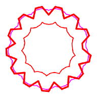
(b) $\varepsilon=\frac{1}{9}\cdot r$, $\delta=\frac{1}{36}\cdot r$

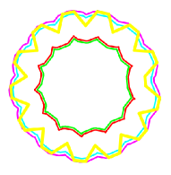
(c) $\varepsilon=\frac{1}{6}\cdot r$, $\delta=\frac{1}{4}\cdot\varepsilon$

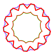
(d) $\varepsilon=\frac{1}{6}\cdot r$, $\delta=\frac{1}{10}\cdot\varepsilon$

Figure 3.1: Dependency of the algorithm outcome on $\varepsilon$ and $\delta$: The input polygon (wheel) appears in bold line. It is colored according to its approximability with the given parameters: green for YES, red for NO and yellow for UNDECIDED. The inset polygon $\widehat{TP}$ and its approximate $(r+\varepsilon)$-offset $\widehat{Q^{\prime}}$ are drawn in green and cyan respectively. Their outer-approximation counterparts are drawn in red and magenta. Figures LABEL:sub@fig:yes_eps and LABEL:sub@fig:no_eps demonstrate how when $\varepsilon$ is tightened from $\frac{1}{3}\cdot r$ to $\frac{1}{9}\cdot r$, with the same $r$ and $\delta$, the decision result changes from YES to NO. The green polygon inside the input polygon in LABEL:sub@fig:yes_eps is a possible $r$-offset solution. The magnification in LABEL:sub@fig:no_eps highlights the area of the input polygon that does not fit inside the outer $\delta$-approximation (in magenta) of maximal possible $(r+\varepsilon)$-offset. Figures LABEL:sub@fig:und_delta and LABEL:sub@fig:no_delta show how when $\delta$ is decreased from $\frac{1}{4}\cdot\varepsilon$ to $\frac{1}{10}\cdot\varepsilon$, for the same $r$ and $\varepsilon$, the decision result changes from UNDECIDED to NO, namely in the latter case the algorithm is able to produce a certified negative answer.

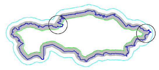
Figure 3.2: A map of Kazakhstan, represented as a polygon $Q$ (in bold blue) with 1881 vertices, is approximable for $\varepsilon=\frac{1}{2}\cdot r$ and $\delta=\frac{1}{8}\cdot\varepsilon$. A solution polygon $P$ (in green) has 335 vertices. Offset($P$,$r$) (shown as lightly-shaded gray $r$-strip around $P$) is inside the $\varepsilon$-offset of the input $Q$ by construction. The $\delta$-approximation of the $\varepsilon$-offset of Offset($P$,$r$) (as computed in line (3) of ApproxDecideInterior ($Q,r,\varepsilon,\delta$)) is drawn in cyan and has 261 vertices. Since the cyan polygon contains $Q$, the Offset($P$,$r$) and $Q$ have Hausdorff distance of at most $\varepsilon$, that is, $Q$ is approximable and $P$ is a solution. Approximability computation took 3.868 seconds in this case on a 3GHz Intel Dual Core processor. The magnification on the left highlights some cavities in the input polygon that have no effect on the Hausdorff distance within this tolerance $\varepsilon$. The magnification on the right demonstrates a sharp end that would prevent $Q$’s approximability with a tighter $\varepsilon$.

4 Searching $\varepsilon$ and $r$

So far, we have assumed that both $r$ and $\varepsilon$ are given as input parameters, and we posed the question of deconstructing a polygon with respect to these parameters. We now investigate three variants where $r$ and/or $\varepsilon$ are unknown. Specifically, we ask, for some input polygon $Q$:

1. Given $r$, what is $\hat{\varepsilon}$, the infimum of all $\varepsilon$-values such that the deconstruction problem has a solution (compare Definition 10)?

2. Given $\varepsilon$, what is the set of radii for which the deconstruction problem has a solution?

3. Given neither $r$ nor $\varepsilon$, how to choose them in a “reasonable” way to obtain a solution?

Whereas the first two questions are formally posed, the third one is of a rather heuristic nature. In all three cases, we also ask for computing some polygonal shape $P$ that approximates the solution of the deconstruction problem for the given set of parameters.

We discuss the posed questions in the remainder of this section. Our main tool will be the decision algorithm for fixed $r$ and $\varepsilon$ as described earlier. Because we aim for a practical algorithm, we formulate our approach using the rational approximation algorithm from Section 3. We have implemented the proposed algorithms; the example at the end of this section has been produced with our implementation.

Searching for $\hat{\varepsilon}$. If we use the exact decision procedure Decide, it is straight-forward to approximate $\hat{\varepsilon}$ to arbitrary precision $\Delta$ employing binary search: Start with the interval $[0,r]$ and choose $\varepsilon$ as the midpoint of the interval. If Decide($Q,r,\varepsilon$) returns YES, recurse on the left subinterval, otherwise, on the right one. Obviously, the interval width is halved in every step, so $O(\log(\frac{r}{\Delta}))$ steps are necessary. Let $\widetilde{\varepsilon_{\Delta}}$ denote the $\hat{\varepsilon}$ approximation, s.t. $\widetilde{\varepsilon_{\Delta}}-\hat{\varepsilon}\leq\Delta$. We demonstrate next that we can achieve the same approximation and produce with it a solution to the deconstruction problem using the rational approximation version ApproxDecide.

Let $|I|$ denote the width of $I$ henceforth on and consider the pseudocode given in Algorithm 5. It computes an interval $I$ of width at most $\Delta$ that contains $\hat{\varepsilon}$.

Algorithm 5 ApproxSearchEps($Q,r,\Delta$)

1. $I\leftarrow[0,r]$

2. while $|I|>\Delta$ do

3. $\varepsilon_{\mathrm{no}}\leftarrow\text{left endpoint of }I$, $\varepsilon_{\mathrm{yes}}\leftarrow\text{right endpoint of }I$

4. $\varepsilon_{\mathrm{mid}}\leftarrow\frac{\varepsilon_{\mathrm{no}}+\varepsilon_{\mathrm{yes}}}{2}$, $\delta\leftarrow\frac{|I|}{8}$

5. $res\leftarrow\textsc{ApproxDecide}(Q,r,\varepsilon_{\mathrm{mid}},\delta)$

6. if $res={\small\sf YES}$ then $I\leftarrow[\varepsilon_{\mathrm{no}},\varepsilon_{\mathrm{mid}}]$

7. otherwise, if $res={\small\sf NO}$, then $I\leftarrow[\varepsilon_{\mathrm{mid}},\varepsilon_{\mathrm{yes}}]$

8. otherwise, ($res={\small\sf UNDECIDED}$), then $I\leftarrow[\varepsilon_{\mathrm{mid}}-\frac{|I|}{4},\varepsilon_{\mathrm{mid}}+\frac{|I|}{4}]$

9. end while

10. return $I$

We prove the invariant that $\hat{\varepsilon}\in I$ after each iteration of the while-loop, implying correctness of the whole algorithm. Trivially, $\hat{\varepsilon}\in[0,r]$, and the invariant is obviously maintained if $\textsc{ApproxDecide}(Q,r,\varepsilon_{\mathrm{mid}},\delta)$ returns YES or NO. For the case of UNDECIDED, recall that ApproxDecide is a combination of the two one-sided approximation algorithms ApproxDecideExterior and ApproxDecideInterior, and both returned UNDECIDED. Theorem 11 and Theorem 13 imply therefore that

$$\frac{|I|}{8}\geq|\frac{\varepsilon_{\mathrm{mid}}-\hat{\varepsilon}}{2}|.$$

It follows that $\hat{\varepsilon}\in[\varepsilon_{\mathrm{mid}}-\frac{|I|}{4},\varepsilon_{\mathrm{mid}}+\frac{|I|}{4}]$ which proves that the invariant is maintained also in this case.

We next compute a solution $P$ for the deconstruction problem for $Q$, $r$ and $\widetilde{\varepsilon_{\Delta}}$. Recall that if ApproxDecide returns YES, the algorithm computes a solution for the deconstruction problem as a by-product. Let $I\leftarrow\textsc{ApproxSearchEps($Q,r,\Delta$)}$ be the approximation interval for $\hat{\varepsilon}$ and let $\varepsilon_{\mathrm{yes}}$ denote the right endpoint of $I$, that is $\hat{\varepsilon}\leq\varepsilon_{\mathrm{yes}}$. We call $\textsc{ApproxDecide}(Q,r,\varepsilon_{\mathrm{yes}},\frac{|I|}{4})$. If the result is YES, then $\widetilde{\varepsilon_{\Delta}}=\varepsilon_{\mathrm{yes}}$ and the polygon computed by ApproxDecide is a solution. Otherwise let us choose $\widetilde{\varepsilon_{\Delta}}=\varepsilon_{\mathrm{yes}}+\frac{\Delta}{2}$ and produce a solution by calling $\textsc{ApproxDecide}(Q,r,\widetilde{\varepsilon_{\Delta}},\frac{\Delta}{8})$. Since the result of $\textsc{ApproxDecide}(Q,r,\varepsilon_{\mathrm{yes}},\frac{|I|}{4})$ was UNDECIDED we conclude from Theorem 11 that $\hat{\varepsilon}\geq\varepsilon_{\mathrm{yes}}-\frac{|I|}{2}$, that is $\widetilde{\varepsilon_{\Delta}}=\varepsilon_{\mathrm{yes}}+\frac{\Delta}{2}$ is indeed $\Delta$-approximation of $\hat{\varepsilon}$. The call to $\textsc{ApproxDecide}(Q,r,\widetilde{\varepsilon_{\Delta}},\frac{\Delta}{8})$ is bound to yield YES because if it returned UNDECIDED, we would have that $\hat{\varepsilon}\geq\widetilde{\varepsilon_{\Delta}}-2\frac{\Delta}{8}=\varepsilon_{\mathrm{yes}}+\frac{\Delta}{4}$, a contradiction to $\hat{\varepsilon}\leq\varepsilon_{\mathrm{yes}}$. So, the polygon computed in this call is a solution.

An overall complexity analysis of approximating $\hat{\varepsilon}$ (and computing a solution) is relatively straightforward: $I$ is obviously halved in every iteration, so it takes $O(\log(\frac{r}{\Delta}))$ iterations to approximate $\hat{\varepsilon}$. Every iteration is bounded by the complexity given in Theorem 16. We omit further details of the proof:

Theorem 17.

Approximating $\hat{\varepsilon}$ to a precision $\Delta>0$ requires

$$O(n\frac{r}{\Delta}\sqrt{\frac{\hat{\varepsilon}}{\Delta}}\cdot\log(n\frac{r}{\Delta}\sqrt{\frac{\hat{\varepsilon}}{\Delta}}))$$

arithmetic operations with rational numbers.

Searching valid radii. We assume now that $Q$ and $\varepsilon$ are given, and discuss the question of what is the set $R$ of radii such that the deconstruction problem has a solution. A priori, it is not clear what is the shape of $R$, but we will prove that it is an interval of the form $[0,r^{*}]$. Having established this, we can apply another variant of binary search to approximate the extremal value $r^{*}$.

In order to prove that $R$ is an interval, we prove first that the deconstruction problem can always be solved for $Q$, $r$ and $\hat{\varepsilon}$. In other words, we can replace the infimum in Definition 10 by a minimum. The proof relies on two properties of infinite intersections of insets and offsets that we show first.

Lemma 18.

Let $(A_{i})_{i\in\mathbb{N}}$ be a sequence of closed sets in $\mathbb{R}^{2}$. Then

$$\mathrm{inset}(\bigcap_{i=0}^{\infty}A_{i},r)=\bigcap_{i=0}^{\infty}\mathrm{inset}(A_{i},r).$$

Proof.

The fact follows readily from the definition of insets: If $a\in\mathrm{inset}(\bigcap_{i=0}^{\infty}A_{i},r)$, then $D_{r}(a)$ is contained in $\bigcap_{i=0}^{\infty}A_{i}$. In particular, it is contained in $A_{i}$ for every $i$ which proves one inclusion. The other direction is similar. ∎

Lemma 19.

Let $(A_{i})_{i\in\mathbb{N}}$ be a sequence of closed sets in $\mathbb{R}^{2}$ with $A_{0}\supseteq A_{1}\supseteq\ldots$. Moreover, let $(\lambda_{i})_{i\in\mathbb{N}}$ be a monotonously decreasing sequence of real numbers that converges to $\lambda\in\mathbb{R}$. Then

$$\mathrm{offset}(\bigcap_{i=0}^{\infty}A_{i},\lambda)=\bigcap_{i=0}^{\infty}\mathrm{offset}(A_{i},\lambda_{i}).$$

Proof.

The “$\subseteq$” inclusion is straight forward, so we concentrate on the “$\supseteq$” part. Fix some $b\in\bigcap\mathrm{offset}(A_{i},\lambda_{i})$. For every $i\in\mathbb{N}$, there exists some $a_{i}\in A_{i}$ such that $(b-a_{i})\in D_{\lambda_{i}}$. Now, the sequence $(b-a_{i})_{i\in\mathbb{N}}$ is a bounded sequence in $\mathbb{R}^{2}$ (bounded by $D_{\lambda_{0}}$) and therefore has a convergent sub-sequence by the well-known Bolzano-Weierstrass Theorem. Let $r$ denote the limit point of this subsequence. In particular, the corresponding subsequence of $(a_{i})_{i\in\mathbb{N}}$ converges to $a:=b-r$. We show that $a\in\bigcap A_{i}$ and $r\in D_{\lambda}$ which suffices to prove the claim.

Assume that $a\notin\bigcap A_{i}$. Then, there is some $n_{0}$ such that $a\notin A_{n_{0}}$. Since $A_{n_{0}}$ is closed, $d(a,A_{n_{0}})=:\varepsilon>0$, where $d$ is the Euclidean distance function. Moreover, because each $A_{n}$ with $n\geq n_{0}$ is included in $A_{n_{0}}$, $d(a,A_{n})\geq\varepsilon$. Because $(a_{i})_{i\in\mathbb{N}}$ converges to $a$, we can find some $N\geq n_{0}$ such that $d(a,a_{N})<\varepsilon$. However, $a_{N}\in A_{N}$, so

$$d(a,A_{N})\leq d(a,a_{N})<\varepsilon=d(a,A_{n_{0}})\leq d(a,A_{N}),$$

which is a contradiction. The fact that $r\in D_{\lambda}$ follows by a similar argument. ∎

Theorem 20.

For arbitrary $Q$ and $r$, and $\hat{\varepsilon}$ as from Definition 10, there exists a solution to the deconstruction problem.

Proof.

Because of Corollary 6, we need to prove that

$$Q\subseteq Q^{\prime}_{\hat{\varepsilon}}:=\mathrm{offset}(\mathrm{inset}(\mathrm{offset}(Q,\hat{\varepsilon}),r),r+\hat{\varepsilon}).$$

Let $(\varepsilon_{i})_{i\in\mathbb{N}}$ be a monotone decreasing sequence of real numbers that converges to $\hat{\varepsilon}$. Because $\varepsilon_{i}>\hat{\varepsilon}$ for each $i$, Decide return YES for each $\varepsilon_{i}$, which is equivalent to

$$Q\subseteq Q^{\prime}_{i}:=\mathrm{offset}(\mathrm{inset}(\mathrm{offset}(Q,\varepsilon_{i}),r),r+\varepsilon_{i}).$$

It is therefore sufficient to prove that

$$Q^{\prime}_{\hat{\varepsilon}}=\bigcap_{i=0}^{\infty}Q^{\prime}_{i}.$$

For that, we apply Lemma 19 on the constant sequence $(Q)_{i\in\mathbb{N}}$ and on $(\varepsilon_{i})_{i\in\mathbb{N}}$ to obtain

$$\mathrm{offset}(Q,\hat{\varepsilon})=\bigcap_{i=0}^{\infty}\mathrm{offset}(Q,\varepsilon_{i}).$$

Applying Lemma 18 yields

$$\mathrm{inset}(\mathrm{offset}(Q,\hat{\varepsilon}),r)=\bigcap_{i=0}^{\infty}(\mathrm{inset}(\mathrm{offset}(Q,\varepsilon_{i}),r),$$

and applying Lemma 19 for the sequences $(\mathrm{inset}(\mathrm{offset}(Q,\varepsilon_{i}),r))_{i\in\mathbb{N}}$ and $(r+\varepsilon_{i})_{i\in\mathbb{N}}$ yields

$$\underbrace{\mathrm{offset}(\mathrm{inset}(\mathrm{offset}(Q,\hat{\varepsilon}),r),r+\hat{\varepsilon})}_{=Q^{\prime}_{\hat{\varepsilon}}}=\bigcap_{i=0}^{\infty}\underbrace{\mathrm{offset}(\mathrm{inset}(\mathrm{offset}(Q,\varepsilon_{i}),r),r+\varepsilon_{i})}_{=Q^{\prime}_{i}}.$$

∎

Since $r$ is no longer fixed, we now consider $\hat{\varepsilon}$ as a function from $\mathbb{R}^{+}$ to $\mathbb{R}^{+}$ depending on $r$; abusing notation, we will let $\hat{\varepsilon}$ by itself denote this function from now on.

Theorem 21.

$\hat{\varepsilon}$ is a monotone increasing function. Moreover, $\hat{\varepsilon}$ is Lipschitz-continuous with Lipschitz factor $1$.

Proof.

We prove monotonicity first: Let $a<b$ denote two radii and $\varepsilon_{a}=\hat{\varepsilon}(a)$, $\varepsilon_{b}=\hat{\varepsilon}(b)$. We will show that Decide $(a,\varepsilon_{b})$ returns YES, which proves that $\varepsilon_{a}\leq\varepsilon_{b}$.

We compare the intermediate results of Decide $(a,\varepsilon_{b})$, denoted by $S_{i}$, to those of Decide $(b,\varepsilon_{b})$, denoted by $B_{i}$:

$$S_{1} =\mathrm{offset}(Q,\varepsilon_{b}) B_{1} =\mathrm{offset}(Q,\varepsilon_{b})=S_{1}$$

$$S_{2} =\mathrm{inset}(S_{1},a) B_{2} =\mathrm{inset}(B_{1},b)=\mathrm{inset}(\mathrm{inset}(S_{1},a),b-a)=\mathrm{inset}(S_{2},b-a)$$

$$S_{3} =\mathrm{offset}(S_{2},a+\varepsilon_{b}) B_{3} =\mathrm{offset}(B_{2},b+\varepsilon_{b})=\mathrm{offset}(\mathrm{offset}(B_{2},b-a),a+\varepsilon_{b})$$

Since

$$\mathrm{offset}(B_{2},b-a)=\mathrm{offset}(\mathrm{inset}(S_{2},b-a),b-a)\subseteq S_{2}$$

it follows that $B_{3}\subseteq S_{3}$. Because Decide $(b,\varepsilon_{b})$ returns YES by definition, it holds that $Q\subseteq B_{3}$, therefore $Q\subseteq S_{3}$ and Decide $(a,\varepsilon_{b})$ also returns YES.

For Lipschitz continuity, let $a<b$ be such that $b-a\leq\delta$, and again $\varepsilon_{a}=\hat{\varepsilon}(a)$, $\varepsilon_{b}=\hat{\varepsilon}(b)$. We show that $\varepsilon_{b}-\varepsilon_{a}\leq\delta$. There exists a polygonal region $P$ that is a solution to the deconstruction problem for $Q$, $a$ and $\varepsilon_{a}$. In other words,

$$H(\mathrm{offset}(P,a),Q)\leq\varepsilon_{a}.$$

Because of the general fact

$$H(A,B)\leq\varepsilon\Rightarrow H(\mathrm{offset}(A,\delta),B)\leq\varepsilon+\delta,$$

and since $b\leq a+\delta$ we have that

$$H(\mathrm{offset}(P,b),Q)\leq H(\mathrm{offset}(P,a+\delta),Q)=H(\mathrm{offset}(\mathrm{offset}(P,a),\delta),Q)\leq\varepsilon_{a}+\delta.$$

Therefore, $P$ is a solution for the deconstruction problem for $Q$, $b$ and $\varepsilon_{a}+\delta$, so $\varepsilon_{b}\leq\varepsilon_{a}+\delta$. ∎

It follows from the monotonicity and Theorem 20 that $R$ is an interval which has $0$ as its left endpoint. Thus, computing $R$ reduces to finding the maximal $r^{*}>0$ such that $\hat{\varepsilon}(r^{*})=\varepsilon$.

Using the exact decision procedure, we can perform a binary search similar to that for approximating $\hat{\varepsilon}$: First, we compute an interval $[0,r]$ containing $r^{*}$. Since $Q$ is finite, we can take $r$ to be the radius of the smallest enclosing circle of $Q$ plus $\varepsilon$. Then, we start the iterative process, deciding on the left or right subinterval depending on the result of Decide for $Q$, $\varepsilon$ and the midpoint of the interval.

What if we are using ApproxDecide instead? Unlike Algorithm 5, we can no longer guarantee that every execution of the approximation algorithm halves the search interval, because a return value UNDECIDED does not bound the distance of the current radius $r$ to the critical value $r^{*}$. Instead, we propose the following scheme: For an interval $I$ with midpoint $r$, ApproxDecide is called with some $\delta$, initially set to $\frac{\varepsilon}{2}$. If it returns UNDECIDED, $\delta$ is divided by $2$ and ApproxDecide is recalled. Eventually, the algorithm returns YES or NO, and the interval $I$ can be halved.

Let $R^{\prime}$ be the preimage of $\varepsilon$ under $\hat{\varepsilon}$. Note that $R^{\prime}$ is an interval (which may consist of only one point). The algorithm from above is guaranteed to converge to some $r\in R^{\prime}$. However, if $R^{\prime}$ contains more than one point, it is not guaranteed to converge to the maximal one (because it gets stuck in an infinite loop as soon as the query value $r$ lies in $R^{\prime}$). One way of avoiding this infinite loops is to decrease $\delta$ only to some threshold and choosing another query value $r$ from the interval if no decision was made. Nevertheless, we have not found an algorithm with the formal guarantee of converging to the largest value in $R^{\prime}$ eventually.

Searching for both $r$ and $\varepsilon$.

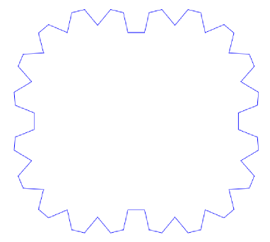
(a) The polygon

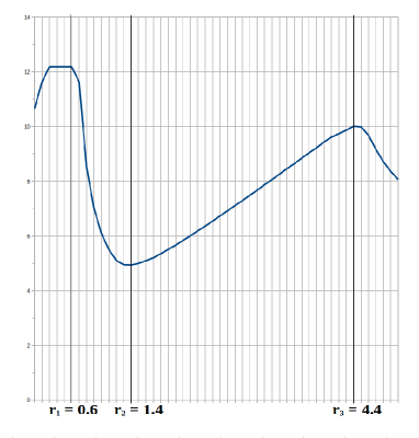
(b) The $J$-graph approximation with $\Delta=\frac{1}{512}$

Figure 4.1: The Flower polygon example: $10$ samples per radius unit for $r\leq 5$.

We finally consider the question of how we can find a reasonable choice of $r$, $\varepsilon$ and a polygonal region $P$, such that $P$ is a solution for the deconstruction problem for $Q$, $r$, and $\varepsilon$. The meaning of “reasonable” depends on the application context, and possible prior information (for instance, a range of possible offset radii). We offer a basic generic approach and justify our choice with an example.

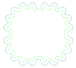
(a) $J$ maximum at $r_{1}=0.6$

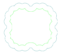
(b) $J$ minimum at $r_{2}=1.4$

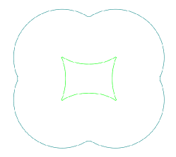
(c) $J$ maximum at $r_{3}=4.4$

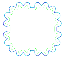
(d) $\widetilde{\varepsilon_{\Delta}}(r_{1})\approx 0.082\cdot r_{1}=0.049\ldots$

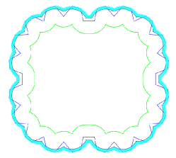
(e) $\widetilde{\varepsilon_{\Delta}}(r_{2})\approx 0.202\cdot r_{2}=0.283\ldots$

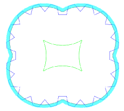
(f) $\widetilde{\varepsilon_{\Delta}}(r_{3})\approx 0.099\cdot r_{3}=0.439\ldots$

Figure 4.2: Flower polygon approximations for the $(r,\widetilde{\varepsilon_{\Delta}}(r))$ values at $J$-graph extrema. In the upper row, approximations of the solutions are shown in green, and their $r$-offsets ($\widetilde{\varepsilon_{\Delta}}(r)$-close to the input) in dark blue. In the lower row the input polygon is shown in blue. The $\widetilde{\varepsilon_{\Delta}}$-width cyan stripe around the $r$-offset demonstrates the quality of the approximation.

Generally, we expect from a reasonable pair $(r,\varepsilon)$ that $\varepsilon$ is small. So, in order to judge whether a good solution exists for radius $r$, we consider $\hat{\varepsilon}(r)$. However, $\hat{\varepsilon}(r)$ being small (or equivalently, $\frac{1}{\hat{\varepsilon}(r)}$ being large) is not a good criterion, because $\hat{\varepsilon}$ is monotone increasing according to Theorem 21, so $r=0$ would always be the best solution. In order to remove the bias towards small radii, we scale the objective function and consider

$$J:\mathbb{R}^{+}\rightarrow\mathbb{R}^{+},r\mapsto\frac{r}{\hat{\varepsilon}(r)}.$$

Note that $J$ is well-defined on the positive axis and continuous. Moreover, we can approximate the graph of $J$ in any finite interval of $r$-values by choosing a sample of the interval and approximating $\hat{\varepsilon}$ at each sample value using Algorithm 5.

We demonstrate by an example that the local maxima of $J$ yield radii that lead to good deconstruction results. Consider the polygonal region defined in Figure 4.1a, and its (approximated) $J$-graph in Figure 4.1b. We can identify two local maxima $r_{1}$ and $r_{3}$; we have plotted the corresponding solutions in Figure 4.2. Indeed, we see that for the large radius $r_{3}$, we obtain a relatively simple solution whose offset blurs away the spikes of $Q$. For the smaller local maximum at $r_{1}$, we obtain a solution with more details such that the spikes can be approximated almost perfectly with the given radius. In contrast, the shape at the local minimum $r_{2}$ combines the disadvantages of the two discussed cases: the solution is similarly complicated as the $r_{1}$-solution (it contains flattened versions of all the spikes), but its approximation quality is not significantly better than for the $r_{3}$ solution which achieves the same with a much larger radius.

5 Deconstructing Convex Polygons

Assume that the input $Q$ to Algorithm 1 is a convex polygon. We first improve the decision algorithm such that it runs in linear time (Algorithm 6). Then we look for a polygon $P$ with a minimal number of vertices ($\mathrm{OPT}$) such that $Q$ is $\varepsilon$-close to $\mathrm{offset}(P,r)$. We give a simple linear-time algorithm that produces a polygon with at most $\mathrm{OPT}+1$ vertices.

Lemma 22.

If $Q$ is a convex polygonal region, then $\Pi$, as computed by Decide  (Algorithm 1), is also a convex polygon, and it can be computed in $O(n)$ time.

Proof.

$Q$ is the intersection of the half-planes bounded by lines that support the polygon edges. Observe that $\Pi$ can be directly constructed from $Q$ by shifting each such line by $r-\varepsilon$ inside the polygon, which shows that $\Pi$ is convex. For the time complexity, we divide the shifted edges of $Q$ into those bounding $Q$ from above, and those bounding $Q$ from below (we assume w.l.o.g. that no edge is vertical). Consider the former edges; the lines supporting those edges have slopes that are monotonously decreasing when traversing the edges from left to right. We have to compute their lower envelope; for that, we dualize by mapping $y=mx+c$ to $(m,-c)$, which preserves above/below relations, and compute the upper hull of the dualized points. Since we already know the order of the points in their $x$-coordinate, this can be done in linear time using Graham’s scan [2, 10]. The same holds for the edges bounding $Q$ from below, taking the upper envelope/lower hull. ∎

Decide first computes $\Pi$ and checks whether $Q\subseteq\mathrm{offset}(\Pi,r+\varepsilon)$. We replace the latter step for convex polygons: Let $q_{1},\ldots,q_{n}$ be the vertices of $Q$ (in counterclockwise order) and define $K_{i}=D_{r+\varepsilon}(q_{i})$, namely the disk of radius $r+\varepsilon$ centered at $q_{i}$. We check whether all these disks intersect $\Pi$:

Algorithm 6 ConvexDecide($Q,r,\varepsilon$)

1. $Q_{\varepsilon}\leftarrow\mathrm{offset}(Q,\varepsilon)$

2. $\Pi\leftarrow\mathrm{inset}(Q_{\varepsilon},r)$

3. if $K_{i}\cap\Pi\neq\emptyset$ for all $i=1,\ldots,n$, return YES,
   otherwise return NO

Lemma 23.

ConvexDecide  agrees with Decide on convex input polygons $Q$ and runs in $O(n)$ time.

Proof.

For correctness, it suffices to prove that $\mathrm{offset}(\Pi,r)$ is $\varepsilon$-close to $Q$ if and only if each $K_{i}$ intersects $\Pi$: Indeed, if any $K_{i}$ does not intersect $\Pi$, then $q_{i}$ has distance more than $r+\varepsilon$ to $\Pi$, so $Q$ is not $\varepsilon$-close to the offset. Otherwise, if each disk $K_{i}$ intersects $\Pi$, $\mathrm{offset}(\Pi,r+\varepsilon)$ contains each vertex of $Q$. Since it is a convex set (as the Minkowski sum of two convex sets), it also covers each edge of $Q$. Thus, $Q\subseteq\mathrm{offset}(\Pi,r+\varepsilon)$, which ensures that $Q$ is $\varepsilon$-close to the offset by Proposition 3.

For the complexity, Lemma 22 shows that the computation of $\Pi$ runs in linear time. We still have to demonstrate that the last step of the algorithm (checking for non-empty intersections) also takes a linear time. Let $e_{1},\ldots,e_{m}$ be the edges of $\Pi$ (with $m<n$). To check for an intersection of $K_{i}$ with $\Pi$, we traverse the edges and check for an intersection, returning NO if no such edge is found. However, if such an edge, say $e_{j}$ was found, we start the search for an intersection of the next disk $K_{i+1}$ at $e_{j}$, again traversing the edges in counterclockwise order. Using this strategy, and noting that $K_{1},\ldots,K_{n}$ are arranged in counterclockwise order around $\Pi$, it can be easily seen that we iterate at most twice through the edges of $\Pi$.∎

Reducing the number of vertices. We assume that $\mathrm{offset}(\Pi,r)$ is $\varepsilon$-close to $Q$. We prefer a simple-looking approximation of $Q$, thus we seek a polygon $P\subseteq\Pi$ whose offset is $\varepsilon$-close to $Q$, but with fewer vertices than $\Pi$. Any such $P$ intersects each of the bulged regions of radius $r+\varepsilon$: $\kappa_{i}:=K_{i}\cap\Pi,i=1,\ldots,n$. We call these bulged regions $\Pi$’s eyelets. The converse is also true: Any convex polygon $P\subseteq\Pi$ that intersects all eyelets $\kappa_{1},\ldots,\kappa_{n}$ has an $r$-offset that is $\varepsilon$-close to $Q$.

The following observation is a simple consequence of Proposition 3:

Proposition 24.

If $\mathrm{offset}(P,r)$ is $\varepsilon$-close to $Q$, and $P\subseteq P^{\prime}\subseteq\Pi$, then $\mathrm{offset}(P^{\prime},r)$ is $\varepsilon$-close to $Q$.

We call a polygonal region $P$ (vertex-)minimal, if its $r$-offset is $\varepsilon$-close to $Q$, and there exists no other such region with fewer vertices. Necessarily, a minimal $P$ must be convex – otherwise, its convex hull $\mathrm{CH}(P)$ has fewer vertices and it can be seen by Proposition 24 that $\mathrm{offset}(\mathrm{CH}(P),r)$ is also $\varepsilon$-close to $Q$. By the next lemma, we can restrict our search to polygons with vertices on $\partial\Pi$.

Lemma 25.

There exists a minimal polygonal region $P\subseteq\Pi$ the vertices of which are all on $\partial\Pi$.

Proof. We pull each vertex $p_{i}\not\in\partial\Pi$ in the direction of the ray emanating from $p_{i-1}$ towards $p_{i}$ until it intersects $\partial\Pi$ in the point $p_{i}^{\prime}$ (dragging $p_{i}$’s incident edges along with it); see the enclosed illustration. For $P^{\prime}=(p_{1},\ldots,p_{i-1},p_{i}^{\prime},p_{i+1},\ldots,p_{m})$: $P\subseteq P^{\prime}\subseteq\Pi$, $\mathrm{offset}(P^{\prime},r)$ is $\varepsilon$-close to $Q$ by Proposition 24.∎

We call a polygonal region $P$ good, if $P\subseteq\Pi$, all vertices of $P$ lie on $\partial\Pi$, and $P$ intersects each eyelet $\kappa_{1},\ldots,\kappa_{n}$. Note that any good $P$ is convex.

Definition 26.

For two points $u,u^{\prime}\in\partial\Pi$, we denote by $[u,u^{\prime}]\subset\partial\Pi$ all points that are met when travelling along $\partial\Pi$ from $u$ to $u^{\prime}$ in counterclockwise order. Likewise, we define half-open and open intervals $[u,u^{\prime})$, $(u,u^{\prime}]$, $(u,u^{\prime})$.

Let $\kappa_{i}=K_{i}\cap\Pi$ be $q_{i}$’s eyelet as before. Consider $\kappa_{i}\cap\partial\Pi$. The portion of that intersection set that is visible from $q_{i}$ (considering $\Pi$ as an obstacle) defines a (ccw-oriented) interval $[v_{i},w_{i}]\subset\partial\Pi$. We call $v_{i}$ the spot of the eyelet $\kappa_{i}$. Finally, for $u,u^{\prime}\in\partial\Pi$, we say that the segment $\overline{{u}{u^{\prime}}}$ is good, if for all spots $v_{i}\in(u,u^{\prime})$, $\overline{{u}{u^{\prime}}}$ intersects the corresponding eyelet $\kappa_{i}$.

The figure above illustrates these definitions: The segment $\overline{{p}{p^{\prime}}}$ is good, whereas $\overline{{p}{p^{\prime\prime}}}$ is not good, because $v_{2}\in(p,p^{\prime\prime})$, but the segment does not intersect $\kappa_{2}$.

Theorem 27.

Let $P$ be a convex polygonal region with all its vertices on $\partial\Pi$. Then, $P$ is good if and only if all its bounding edges are good.

Proof.

We first prove that if all the edges of $P$ are good, then $P$ is good. It suffices to argue that it intersects all eyelets $\kappa_{1},\ldots,\kappa_{n}$. Let $p_{1},\ldots,p_{k}$ be the vertices of $P$ in counterclockwise order. Any spot $v_{i}$ of an eyelet $\kappa_{i}$ either corresponds to some vertex $p_{\ell}$ of $P$, or lies inside some interval $(p_{\ell},p_{\ell+1})$. Since $\overline{{p_{\ell}}{p_{\ell+1}}}$ is good, it intersects $\kappa_{i}$.

For the converse, assume that $\overline{{p_{\ell}}{p_{\ell+1}}}$ is not good, which encloses with the interval $(p_{\ell},p_{\ell+1})$ a polygonal region $R\subseteq\Pi\setminus P$. Hence, there is a spot $v_{i}\in R$ such that $\overline{{p_{\ell}}{p_{\ell+1}}}$ does not intersect the eyelet $\kappa_{i}$. It follows that the entire $\kappa_{i}$ is inside $R$ (see the illustration above, considering $\overline{{p}{p^{\prime\prime}}}$ and $\kappa_{2}$). Thus, $P\cap\kappa_{i}=\emptyset$, and so $P$ cannot be good. ∎

For $u\in\partial\Pi$, we define its horizon $h_{u}\in\partial\Pi$ as the maximal point in counterclockwise direction such that that segment $\overline{{u}{h_{u}}}$ is good. Consider again the figure above: The segment $\overline{{p}{h_{p}}}$ is tangential to $\kappa_{2}$, so if going any further than $h_{p}$ on $\partial\Pi$ from $p$, the segment would miss $\kappa_{2}$ and thus become non-good.

Lemma 28.

Let $P$ be a good polygonal region, and $u\in\partial\Pi$. Then, $P$ has a vertex $p\in(u,h_{u}]$.

Proof.

Assume to the contrary that $P$ has no such vertex, and let $p_{1},\ldots,p_{\ell}$ be its vertices on $\partial\Pi$. Let $p_{j}$ be the vertex of $P$ such that $u\in(p_{j},p_{j+1})$. Then, also $h_{u}\in(p_{j},p_{j+1})$, because otherwise, $p_{j+1}\in(u,h_{u}]$. Since $P$ is good, the segment $\overline{{p_{j}}{p_{j+1}}}$ is good, too. It is not hard to see that, consequently, both $\overline{{p_{j}}{u}}$ and $\overline{{u}{p_{j+1}}}$ are good. However, the latter contradicts the maximality of the horizon $h_{u}$. ∎

For an arbitrary initial vertex $s\in\partial\Pi$, we finally specify a polygonal region $P^{s}$ by iteratively defining its vertices. Set $p_{1}:=s$. For any $j\geq 1$, if the segment $\overline{{p_{j}}{s}}$, which would close $P^{s}$, is good, stop. Otherwise, set $p_{j+1}:=h_{p_{j}}$. Informally, we always jump to the next horizon until we can reach $s$ again without missing any of the eyelets. By construction, all segments of $P^{s}$ are good, so $P^{s}$ itself is good. The (almost-)optimality of this construction mainly follows from Lemma 28.

Theorem 29.

Let $P$ be a minimal polygonal region for $Q$, having $\mathrm{OPT}$ vertices. Then, for any $s\in\partial\Pi$, $P^{s}$ has at most $\mathrm{OPT}+1$ vertices.

Proof.

We first prove that $P^{s}$ has the minimal number of vertices among all good polygonal regions that have $s$ as a vertex. Let $s:=p_{1},\ldots,p_{m}$ be the vertices of $P^{s}$. There are $m-1$ segments of the form $\overline{{p_{\ell}}{h_{p_{\ell}}}}$. By Lemma 28, any good polygonal region has a vertex inside each of the intervals $(p_{\ell},h_{p_{\ell}}]$. Together with the vertex at $s$, this yields at least $m$ vertices, thus $P^{s}$ is indeed minimal among these polygonal regions.

Next, consider any minimal polygonal region $P^{\star}$. We can assume that all its vertices are on $\partial\Pi$ by Lemma 25. If $s$ is not a vertex of $P^{\star}$, we add it to the vertex set and obtain a polygonal region $P^{\prime}$ with at most $\mathrm{OPT}+1$ vertices that has $s$ as a vertex. $P^{s}$ has at most as many vertices as $P^{\prime}$, so $m\leq\mathrm{OPT}+1$. ∎

As each visit of an eyelet requires constant time, the construction of a horizon is proportional to the number of visited eyelets, and there are only linearly many eyelets. Thus, we can state:

Theorem 30.

For an arbitrary initial vertex $s$, computing $P^{s}$ requires $O(n)$ time.

Proof.

We prove that computing the horizon of a point $u$ takes a number of operations proportional to the number of eyelets that are visited by the segment $\overline{{u}{h_{u}}}$. Let us consider an arbitrary $u\in\partial\Pi$. By rotating appropriately, we can assume, without loss of generality, that $u$ lies on a vertical edge of $\Pi$ (or, if $u$ is a vertex, that the next edge in counterclockwise order is vertical), and that the edge is traversed top-down. The horizon is determined by the slope of the edge at $u$. Note that for each eyelet $\kappa_{1},\ldots,\kappa_{n}$, there is an interval of slopes $I_{1}^{(u)},\ldots,I_{n}^{(u)}$ such that the segment from $u$ with slope $\lambda$ intersects $\kappa_{i}$ if and only if $\lambda\in I_{i}^{(u)}$. Furthermore, each single $I_{i}^{(u)}$ can be computed with a constant number of arithmetic operations. Assuming that the next eyelet to be travelled from the current $p_{i}$ is $\kappa_{j}$, we can iteratively compute the intersections $I_{j}\cap I_{j+1}\cap I_{j+2},\ldots$ until $I_{j}\cap\ldots\cap I_{j+k}$ is empty. In this case, we choose $\lambda_{i}:=\max(I_{j}\cap\ldots\cap I_{j+k-1})$ as the slope for the next segment, which must be $\overline{{p_{i}}{h_{p_{i}}}}$ since it is good by construction, and any larger slope would produce a non-good segment. Based on this property, it is easy to show that computing $P^{s}$ needs a number of operations which is proportional to $n$, the number of eyelets. ∎

6 Open Problems

We have shown how to decide whether a given arbitrary polygonal shape $Q$ is composable as the Minkowski sum of another polygonal region and a disk of radius $r$, up to some tolerance $\varepsilon$. Many related questions remain open. (i) Deconstruction of Minkowski sums seems more difficult when both summands are more complicated than a disk; many practical scenarios may raise this general deconstruction problem. (ii) It would be interesting to analyze the deconstruction not only under the Hausdorff distance but for other similarity measures, such as the Frêchet or the symmetric distance. (iii) Can one remove the extra vertex when seeking an optimal (vertex minimal) polygonal summand $P$ in the convex case. (iv) Finding an optimal or near-optimal polygonal summand in the non-convex case seems challenging. (v) As in polygonal simplification, we could also search for the polygonal region with a given number of vertices whose $r$-offset minimizes the (Hausdorff) distance to the given shape. (vi) The offset-deconstruction problem can be reformulated in higher dimensions. We consider especially the three-dimensional case to be of practical relevance.

References

- [1] A. Aggarwal, H. Booth, J. O’Rourke, S. Suri, and C.-K. Yap. Finding minimal convex nested polygons. Inf. Comput., 83(1):98–110, 1989.
- [2] A. M. Andrew. Another efficient algorithm for convex hulls in two dimensions. Inform. Process. Lett., 9(5):216–219, 1979.
- [3] J. Canny, B. Donald, and E. K. Ressler. A rational rotation method for robust geometric algorithms. In SCG ’92: Proceedings of the Eighth Annual Symposium on Computational geometry, pages 251–260, New York, NY, USA, 1992. ACM.
- [4] J. Damen, M. van Kreveld, and B. Spaan. High quality building generalization by extending the morphological operators. In 11th ICA Workshop on Generalisation and Multiple Reslides, June 2008.
- [5] R. Drysdale, G. Rote, and A. Sturm. Approximation of an open polygonal curve with a minimum number of circular arcs and biarcs. Computational Geometry, Theory and Applications, 41(1-2):31 – 47, 2008.
- [6] Ioannis Emiris and Elias Tsigaridas. Algebraic geometry and geometric modeling, chapter Minkowski decomposition of convex lattice polygons, pages 217–236. Springer, 2006.
- [7] Efi Fogel, Ron Wein, Baruch Zukerman, and Dan Halperin. 2D regularized Boolean set-operations. In CGAL User and Reference Manual. CGAL Editorial Board, 3.7 edition, 2010. http://www.cgal.org/Manual/3.7/doc_html/cgal_manual/packages.html#Pkg:BooleanSetOperations2.
- [8] S. Gao and A.G.B Lauder. Decomposition of polytopes and polynomials. Discrete & Computational Geometry, 26:89–104, 2001.
- [9] Geert-Jan Giezeman and Wieger Wesselink. 2D polygons. In CGAL User and Reference Manual. CGAL Editorial Board, 3.7 edition, 2010. http://www.cgal.org/Manual/3.7/doc_html/cgal_manual/packages.html#Pkg:Polygon2.
- [10] R. L. Graham. An efficient algorithm for determining the convex hull of a finite planar set. Inform. Process. Lett., 1:132–133, 1972.
- [11] Allan Hansen and Farhad Arbab. An algorithm for generating NC tool paths for arbitrarily shaped pockets with islands. ACM Trans. Graph., 11:152–182, April 1992.
- [12] M. Heimlich and M. Held. Biarc approximation, simplification and smoothing of polygonal curves by means of Voronoi-based tolerance bands. Int. J. Comput. Geometry Appl., 18(3):221–250, 2008.
- [13] Martin Held. On the Computational Geometry of Pocket Machining, volume 500 of Lecture Notes in Computer Science. Springer, 1991.
- [14] K. Kedem, R. Livne, J. Pach, and M. Sharir. On the union of Jordan regions and collision-free translational motion amidst polygonal obstacles. Discrete & Computational Geometry, 1(1):59–71, 1986.
- [15] Daniel Leven and Micha Sharir. Planning a purely translational motion for a convex object in two-dimensional space using generalized Voronoi diagrams. Discrete & Computational Geometry, 2:9–31, 1987.
- [16] Georges Matheron. Random sets and integral geometry. Wiley New York,, 1974.
- [17] A.M. Ostrowski. Über die Bedeutung der Theorie der konvexen Polyeder für die formale Algebra. Jahresberichte Deutsche Math. Ver., 30:98–99, 1921. English version: “On the Significance of the Theory of Convex Polyhedra for Formal Algebra” ACM Sigsam Bulletin 33 (1999).
- [18] F. P. Preparata and M. I. Shamos. Computational Geometry: An Introduction. Springer-Verlag, 3rd edition, October 1990.
- [19] G. T. Sallee. Minkowski decomposition of convex sets. Israel Journal of Mathematics, 12(3):266–276, September 1982.
- [20] Jean Serra. Image Analysis and Mathematical Morphology. Academic Press, Inc., Orlando, FL, USA, 1983.
- [21] Ron Wein. 2D Minkowski sums. In CGAL User and Reference Manual. CGAL Editorial Board, 3.7 edition, 2010. http://www.cgal.org/Manual/3.7/doc_html/cgal_manual/packages.html#Pkg:MinkowskiSum2.
- [22] Chee-Keng Yap. An algorithm for the Voronoi diagram of a set of simple curve segments. Discrete & Computational Geometry, 2:365–393, 1987.