Abstract

Within the framework of quantum electrodynamics (QED), vacuum is a nonlinear medium which can be linearized for a rapidly time-varying electromagnetic field with a small amplitude subjected to a magnetostatic field. The linearized QED vacuum is a uniaxial dielectric-magnetic medium for which the degree of anisotropy is exceedingly small. By implementing an affine transformation of the spatial coordinates, the degree of anisotropy may become sufficiently large as to be readily perceivable. The inverse Bruggeman formalism can be implemented to specify a homogenized composite material (HCM) which is electromagnetically equivalent to the affinely transformed QED vacuum. This HCM can arise from remarkably simple component materials; for example, two isotropic dielectric materials and two isotropic magnetic materials, randomly distributed as oriented spheroidal particles.

Keywords: quantum electrodynamics, vacuum birefringence, homogenization, inverse Bruggeman formalism

1 Introduction

Classical vacuum is a linear medium for which the principle of superposition holds. Consequently, light propagation in classical vacuum is unaffected by the presence of a magnetostatic field. However, within the framework of quantum electrodynamics (QED), vacuum is a nonlinear medium [1]. The QED vacuum can be linearized for a rapidly time-varying electromagnetic field with a small amplitude subjected to a slowly varying (or static) magnetic field [2]. A consequence of linearization is that the QED vacuum appears as a uniaxial dielectric–magnetic medium for optical fields [3]. The constitutive parameters which characterize this uniaxial medium depend on the magnitude and direction of the magnetostatic field.

The degree of anisotropy associated with the QED vacuum is exceedingly small. Consequently, a direct measurement of this attribute poses enormous challenges to experimentalists [4], and experimental verification of the anisotropy of the QED vacuum is eagerly awaited [5]. In view of this difficulty, we propose an experimental simulation of the QED vacuum which would enable the anisotropy to be explored for practicable magnetostatic fields. The simulation is based on a homogenized composite material (HCM), which arises from the homogenization of remarkably simple component materials. For example, the component materials could be isotropic dielectric and magnetic materials, randomly distributed as oriented spheroidal particles. Similar HCM-based simulations have recently been described for the Schwarzschild-(anti-)de Sitter spacetime [6] and cosmic strings [7].

In the following sections, 3-vectors are underlined with the addition of the $\hat{}$ symbol denoting a unit vector. Double underlining indicates a 3$\times$3 dyadic with the dyadic transpose being labelled with the additional ^T symbol. The 3$\times$3 identity dyadic represented as $\underline{\underline{I}}$. The permittivity and permeability of classical vacuum are written as $\epsilon_{0}=8.854\times 10^{-12}$ F m^-1 and $\mu_{0}=4\pi\times 10^{-7}$ H m^-1, respectively.

2 Electrodynamics of QED vacuum

We consider vacuum under the influence of a magnetostatic field ${\underline{B}}_{s}=|{\underline{B}}_{s}|\,\hat{{\underline{B}}}_{s}$. In classical vacuum, the passage of light is unaffected by ${\underline{B}}_{s}$, as reported by an inertial observer. However, this is not the case for the QED vacuum. The QED vacuum is a nonlinear medium which can be linearized for rapidly time–varying plane waves. Thereby, for propagation of light, QED vacuum is represented by the anisotropic dielectric–magnetic constitutive relations [3]

$$\left.\begin{array}[]{l}{\underline{D}}=\epsilon_{0}\underline{\underline{\epsilon}}\mbox{ \tiny{${}^{\bullet}$} }{\underline{E}\vspace{4pt}}\\ {\underline{B}}=\mu_{0}\underline{\underline{\mu}}\mbox{ \tiny{${}^{\bullet}$} }{\underline{H}}\end{array}\right\}.$$ (1)

The relative permittivity and relative permeability dyadics of the QED vacuum have the uniaxial forms [8]

$$\left.\begin{array}[]{l}\underline{\underline{\epsilon}}=\left(1-8a|{\underline{B}}_{s}|^{2}\right)\left(\underline{\underline{I}}-\hat{{\underline{B}}}_{s}\hat{{\underline{B}}}_{s}\right)+\left(1+20a|{\underline{B}}_{s}|^{2}\right)\hat{{\underline{B}}}_{s}\hat{{\underline{B}}}_{s}\vspace{8pt}\\ \underline{\underline{\mu}}=\displaystyle{\frac{1}{1-8a|{\underline{B}}_{s}|^{2}}\left(\underline{\underline{I}}-\hat{{\underline{B}}}_{s}\hat{{\underline{B}}}_{s}\right)+\frac{1}{1-24a|{\underline{B}}_{s}|^{2}}\hat{{\underline{B}}}_{s}\hat{{\underline{B}}}_{s}}\end{array}\right\},$$ (2)

where the constant $a=6.623\times 10^{-26}\,{\mbox{H}}^{-1}~{}{\mbox{kg}}^{-1}\,\,{\mbox{m}}^{2}\,\,{\mbox{s}}^{2}$. The constitutive dyadics (2) were derived by Adler [3] from the Heisenberg–Euler effective Lagrangrian of the electromagnetic field [9, 10].

Since $a$ is exceedingly small, the value of $a|{\underline{B}}_{s}|^{2}$ is also exceedingly small in comparison with unity for typical values of $|{\underline{B}}_{s}|$. For example, in the PVLAS experiment $|{\underline{B}}_{s}|=5$ T typically [5], which yields $a|{\underline{B}}_{s}|^{2}=1.656\times 10^{-24}$. Accordingly, the degree of anisotropy represented by the constitutive dyadics (2) is also exceedingly small. In order to achieve degrees of anisotropy that could be realistically attained in a controlled manner for a practical simulation of QED vacuum, we implement the affine transformation

$${\underline{x}}\mapsto{\underline{x}}^{\prime}\equiv\underline{\underline{J}}\mbox{ \tiny{${}^{\bullet}$} }{\underline{x}}$$ (3)

of the spatial coordinates. The transformation dyadic

$$\underline{\underline{J}}=p\,\left(\underline{\underline{I}}-\hat{{\underline{B}}}_{s}\hat{{\underline{B}}}_{s}\right)+q\,\hat{{\underline{B}}}_{s}\hat{{\underline{B}}}_{s}$$ (4)

employs

$$\left.\begin{array}[]{l}\displaystyle{p=\sqrt{\frac{\left(1-8a|{\underline{B}}_{s}|^{2}\right)\left(1+20a|{\underline{B}}_{s}|^{2}\right)}{\left(1-2\delta|{\underline{B}}_{s}|\right)\left(1+5\delta|{\underline{B}}_{s}|\right)}}\vspace{8pt}}\\ \displaystyle{q=\frac{1-8a|{\underline{B}}_{s}|^{2}}{1-2\delta|{\underline{B}}_{s}|}}\end{array}\right\}$$ (5)

and the scalar parameter $\delta>0$. For definiteness, we fix $\delta=0.02$. Thus, the affine-transformed relative permittivity and permeability dyadics are given as [11]

$$\underline{\underline{\epsilon}}^{\prime} \equiv \frac{1}{\det\underline{\underline{\epsilon}}}\,\underline{\underline{J}}\mbox{ \tiny{${}^{\bullet}$} }\underline{\underline{\epsilon}}\mbox{ \tiny{${}^{\bullet}$} }\underline{\underline{J}}^{T}$$ (6)

$$= \left(1-2\delta|{\underline{B}}_{s}|\right)\left(\underline{\underline{I}}-\hat{{\underline{B}}}_{s}\hat{{\underline{B}}}_{s}\right)+\left(1+5\delta|{\underline{B}}_{s}|\right)\hat{{\underline{B}}}_{s}\hat{{\underline{B}}}_{s}$$ (7)

$$\equiv \epsilon^{\prime}_{t}\left(\underline{\underline{I}}-\hat{{\underline{B}}}_{s}\hat{{\underline{B}}}_{s}\right)+\epsilon^{\prime}_{s}\hat{{\underline{B}}}_{s}\hat{{\underline{B}}}_{s}$$ (8)

and

$$\underline{\underline{\mu}}^{\prime} \equiv \frac{1}{\det\underline{\underline{\mu}}}\,\underline{\underline{J}}\mbox{ \tiny{${}^{\bullet}$} }\underline{\underline{\mu}}\mbox{ \tiny{${}^{\bullet}$} }\underline{\underline{J}}^{T}$$ (9)

$$= \frac{1-2\delta|{\underline{B}}_{s}|}{\left(1-8a|{\underline{B}}_{s}|^{2}\right)^{2}}\,\left(\underline{\underline{I}}-\hat{{\underline{B}}}_{s}\hat{{\underline{B}}}_{s}\right)+\frac{1+5\delta|{\underline{B}}_{s}|}{1-4a|{\underline{B}}_{s}|^{2}\left(1+120a|{\underline{B}}_{s}|^{2}\right)}\,\hat{{\underline{B}}}_{s}\hat{{\underline{B}}}_{s}$$ (10)

$$\equiv \mu^{\prime}_{t}\left(\underline{\underline{I}}-\hat{{\underline{B}}}_{s}\hat{{\underline{B}}}_{s}\right)+\mu^{\prime}_{s}\hat{{\underline{B}}}_{s}\hat{{\underline{B}}}_{s}.$$ (11)

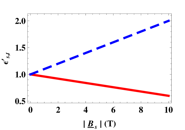
Figure 1: The relative permittivity parameters $\epsilon^{\prime}_{s}$ (blue, dashed) and $\epsilon^{\prime}_{t}$ (red, solid) plotted versus $|{\underline{B}}_{\,s}|$ (T).

Notice that for the range $|{\underline{B}}_{s}|\in\left(0,10\right)$ T, the denominators of both terms on the right side of Eq. (10) are both approximately equal to unity, and therefore $\underline{\underline{\epsilon}}^{\prime}\approx\underline{\underline{\mu}}^{\prime}$. The components $\epsilon^{\prime}_{s}$ and $\epsilon^{\prime}_{t}$ are linearly dependent upon $|{\underline{B}}_{s}|$, as illustrated in Fig. 1. The plots of $\mu^{\prime}_{s,t}$ versus $|{\underline{B}}_{s}|$ are practically identical to those of $\epsilon^{\prime}_{s,t}$.

3 Simulation as a homogenized composite material

Let us now turn to the question: How can one specify an HCM which is a uniaxial dielectric-magnetic material with relative permittivity dyadic $\underline{\underline{\epsilon}}_{\,HCM}\equiv\underline{\underline{\epsilon}}^{\prime}$ and relative permeability dyadic $\underline{\underline{\mu}}_{\,HCM}\equiv\underline{\underline{\mu}}^{\prime}$? In order to answer this question, we make use of the well-established Bruggeman homogenization formalism [12, 13].

Suppose we consider the homogenization of four component materials, labelled $a$, $b$, $c$ and $d$. Two of the components ($a$ and $b$, say) are isotropic dielectric materials while the other two ($c$ and $d$) are isotropic magnetic materials. Thus, the component materials are specified by

• the relative permittivities $\epsilon_{a}$, $\epsilon_{b}$, $\epsilon_{c}$ and $\epsilon_{d}$, with $\epsilon_{c}=\epsilon_{d}=1$; and

• the relative permeabilities $\mu_{a}$, $\mu_{b}$, $\mu_{c}$ and $\mu_{d}$, with $\mu_{a}=\mu_{b}=1$.

The four component materials are randomly distributed with volume fractions $f_{a}$, $f_{b}$, $f_{c}$, $f_{d}\in\left(0,1\right)$, with $f_{d}=1-f_{a}-f_{b}-f_{c}$. All four component materials consist of identically oriented spheroidal particles. The symmetry axis for all these spheroidal particles lies parallel to $\hat{{\underline{B}}}_{s}$. Accordingly, the surface of each spheroid relative to its centre is prescribed by the vector

$${\underline{r}}_{\,s}=\rho_{\ell}\,\underline{\underline{U}}_{\,\ell}\cdot\hat{{\underline{r}}},$$ (12)

wherein the shape dyadic

$$\underline{\underline{U}}_{\,\ell}=\left(\underline{\underline{I}}-\hat{{\underline{B}}}_{s}\hat{{\underline{B}}}_{s}\right)+U_{\ell}\hat{{\underline{B}}}_{s}\hat{{\underline{B}}}_{s},\qquad\qquad\left(\ell=a,b,c,d\right),$$ (13)

is real symmetric [14] and positive definite, the radial unit vector is $\hat{{\underline{r}}}$, and the linear measure $\rho_{\ell}$ is required to be small compared to the electromagnetic wavelengths under consideration. The shape parameter $U_{\ell}>1$ for prolate spheroids and $0<U_{\ell}<1$ for oblate ones.

Under the Bruggeman homogenization formalism, the corresponding HCM is a uniaxial dielectric-magnetic material, specified by relative permittivity and permeability dyadics of the form

$$\underline{\underline{\tau}}_{\,HCM}=\tau^{HCM}_{t}\left(\underline{\underline{I}}-\hat{{\underline{B}}}_{s}\hat{{\underline{B}}}_{s}\right)+\tau^{HCM}_{s}\hat{{\underline{B}}}_{s}\hat{{\underline{B}}}_{s},\qquad\left(\tau=\epsilon,\mu\right).$$ (14)

For the particular case of the uniaxial dielectric-magnetic HCM involved here, full details of the numerical process of computing the dyadics $\underline{\underline{\epsilon}}_{\,HCM}$ and $\underline{\underline{\mu}}_{\,HCM}$, from a knowledge of $\epsilon_{a,b,c,d}$, $\mu_{a,b,c,d}$, $U_{a,b,c,d}$ and $f_{a,b,c,d}$, are provided elsewhere [6].

Conventionally, homogenization formalisms are used to estimate the constitutive parameters of HCMs, based on a knowledge of the constitutive and morphological parameters of their component materials and their volume fractions. In contrast, here our goal is to estimate the constitutive and morphological parameters as well as the volume fractions of the component materials which give rise to a HCM such that $\underline{\underline{\epsilon}}_{\,HCM}$ coincides with $\underline{\underline{\epsilon}}^{\prime}$ and $\underline{\underline{\mu}}_{\,HCM}$ coincides with $\underline{\underline{\mu}}^{\prime}$. We do so via an inverse implementation of the Bruggeman formalism. Formal expressions of the inverse Bruggeman formalism are available [15], but in some instances these can be ill-defined [16]. In practice, the inverse formalism may be more effectively implemented by direct numerical methods [17]. Note that certain constitutive parameter regimes have been identified as problematic for the inverse Bruggeman formalism [18], but these regimes are not the same as those considered here.

We consider the following three different implementations of the inverse Bruggeman formalism. In each implementation, four scalar parameters are to be determined.

• The relative permittivities $\epsilon_{a,b}$ and the relative permeabilities $\mu_{c,d}$ are assumed to be known, and all spheroidal particles have the same shape, i.e., $U_{a}=U_{b}=U_{c}=U_{d}\equiv U$. We then determine the common shape parameter $U$ and the volume fractions $f_{a}$, $f_{b}$ and $f_{c}$.

• The relative permittivities $\epsilon_{a,b}$ and the relative permeabilities $\mu_{c,d}$ are assumed to be known, and the volume fractions $f_{a,b,c}$ are fixed. We then determine the shape parameters $U_{a}$, $U_{b}$, $U_{c}$ and $U_{d}$.

• The shape parameters $U_{a,b,c,d}$ and the volume fractions $f_{a,b,c}$ are fixed. We then determine the relative permittivities $\epsilon_{a,b}$ and relative permeabilities $\mu_{c,d}$.

To describe the inversion of the Bruggeman formalism, let us focus on implementation I as a representative example, the inversion processes for implementations II and III being analogous. Suppose that $\left\{\breve{\epsilon}^{HCM}_{s},\breve{\epsilon}^{HCM}_{t},\breve{\mu}^{HCM}_{s},\breve{\mu}^{HCM}_{t}\right\}$ are forward Bruggeman estimates of the HCM’s relative permittivity and relative permeability parameters which are computed for physically reasonable ranges of the parameters $U$ and $f_{a,b,c}$; i.e., $U\in\left(U^{-},U^{+}\right)$ and $f_{a,b,c}\in\left(f^{-}_{a,b,c},f^{+}_{a,b,c}\right)$. Next:

• Let $f_{a}=\left(f^{-}_{a}+f^{+}_{a}\right)/2$, $f_{b}=\left(f^{-}_{b}+f^{+}_{b}\right)/2$, and $f_{c}=\left(f^{-}_{c}+f^{+}_{c}\right)/2$. For all $U\in\left(U^{-},U^{+}\right)$, determine the value $U^{\dagger}$ which yields the minimum value of the scalar quantity

  $$\Delta = \Big{[}\left(\frac{\breve{\epsilon}^{HCM}_{s}-\epsilon^{\prime}_{s}}{\epsilon^{\prime}_{s}}\right)^{2}+\left(\frac{\breve{\epsilon}^{HCM}_{t}-\epsilon^{\prime}_{t}}{\epsilon^{\prime}_{t}}\right)^{2}+\left(\frac{\breve{\mu}^{HCM}_{s}-\mu^{\prime}_{s}}{\mu^{\prime}_{s}}\right)^{2}+\left(\frac{\breve{\mu}^{Br}_{t}-\mu^{\prime}_{t}}{\mu^{\prime}_{t}}\right)^{2}\Big{]}^{1/2}.$$ (15)

• Let $U=U^{\dagger}$, $f_{b}=\left(f^{-}_{b}+f^{+}_{b}\right)/2$, and $f_{c}=\left(f^{-}_{c}+f^{+}_{c}\right)/2$. For all $f_{a}\in\left(f_{a}^{-},f_{a}^{+}\right)$, determine the value $f_{a}^{\dagger}$ which yields the minimum value of $\Delta$.

• Let $U=U^{\dagger}$, $f_{a}=f_{a}^{\dagger}$, and $f_{c}=\left(f^{-}_{c}+f^{+}_{c}\right)/2$. For all $f_{b}\in\left(f_{b}^{-},f_{b}^{+}\right)$, determine the value $f_{b}^{\dagger}$ which yields the minimum value of $\Delta$.

• Let $U=U^{\dagger}$, $f_{a}=f_{a}^{\dagger}$, and $f_{b}=f_{b}^{\dagger}$. For all $f_{c}\in\left(f_{c}^{-},f_{c}^{+}\right)$, determine the value $f_{c}^{\dagger}$ which yields the minimum value of $\Delta$.

The steps (1)–(4) are then repeated, with $f_{a}^{\dagger}$, $f_{b}^{\dagger}$, and $f_{c}^{\dagger}$ being the fixed values of $f_{a,b,c}$ in step (1), $f_{b}^{\dagger}$ and $f_{c}^{\dagger}$ being the fixed values of $f_{b,c}$ in step (2), and $f_{c}^{\dagger}$ being the fixed value of $f_{c}$ in step (3), until the value of $\Delta$ becomes acceptably small.

4 Numerical illustrations

Numerical illustrations of the implementations I–III are provided in Figs. 2–4. For all results presented, the degree of convergence of the numerical schemes which provide the inverse Bruggeman estimates was $<1\%$, and in most instances this value was $<0.1\%$.

• For Fig. 2, the constitutive parameters of the component materials were taken to be $\epsilon_{a}=4$, $\epsilon_{b}=0.3$, $\mu_{c}=3.4$ and $\mu_{d}=0.4$. The computed common shape parameter $U$ and volume fractions $f_{a,b,c}$ are plotted versus $|{\underline{B}}_{s}|$. While the volume fractions vary little as $|{\underline{B}}_{s}|$ is increased from 1 to 2.5 T, the common shape parameter increases exponentially.

• The constitutive parameters of the component materials were again taken to be $\epsilon_{a}=4$, $\epsilon_{b}=0.3$, $\mu_{c}=3.4$ and $\mu_{d}=0.4$ for Fig. 3. In addition, the volume fractions were fixed at $f_{a}=0.15$, $f_{b}=0.25$ and $f_{c}=0.21$. The computed four shape parameters $U_{a,b,c,d}$ are plotted versus $|{\underline{B}}_{s}|$. All four shape parameters increase uniformly as $|{\underline{B}}_{s}|$ is increased from 1 to 2 T. This reflects the fact that the degree of anisotropy of the HCM is required to increase as $|{\underline{B}}_{s}|$ increases.

• Lastly, in Fig. 4 the common shape parameter is fixed at $U=5$ while the volume fractions are fixed at $f_{a,b,c}=2.5$. The computed constitutive parameters $\epsilon_{a,b}$ and $\mu_{c,d}$ are plotted versus $|{\underline{B}}_{s}|$. In this case, $\epsilon_{a}$ turns out to be approximately the same as $\mu_{c}$. And similarly $\epsilon_{b}$ turns out to be approximately the same as $\mu_{d}$. While $\epsilon_{a}$ and $\mu_{c}$ decrease uniformly as $|{\underline{B}}_{s}|$ is increased from 1 to 3 T, the opposite is true of $\epsilon_{b}$ and $\mu_{d}$.

5 Closing remarks

By means of the inverse Bruggeman formalism, an HCM may be specified which is electromagnetically equivalent to the QED vacuum subject to a spatial affine transformation. The affinely transformed QED vacuum retains the same uniaxial dielectric-magnetic form as the un-transformed QED vacuum, but the degee of anisotropy is greatly exaggerated by means of the affine transformation. By reversing the transformation represented by eq. (3), the properties of QED vacuum may be inferred from those of the HCM.

For illustration, the inverse homogenization formulation presented here was based on four isotropic component materials. However, the desired HCM could also be realized by alternative inverse homogenization formulations. For example, the HCM could arise from only two component materials. These two components materials could be either both isotropic dielectric-magnetic materials distributed as oriented spheroidal particles or both uniaxial dielectric-magnetic materials (with parallel symmetry axes) distributed as spherical particles [13, 19]. However, the four-component formulation presented here involves the simplest of component materials and allows a large degree of freedom in choosing their constitutive parameters.

Finally, let us note that the relative permittivities and relative permeabilities of the component materials needed for the HCM, as presented in Figs. 2–4, are not at all infeasible. Indeed, present-day technology allows for the possibility of materials with a considerably wider range of constitutive parameters to be engineered [20, 21, 22].

Acknowledgment: AL thanks the Charles Godfrey Binder Endowment at Penn State for partial financial support of his research activities.

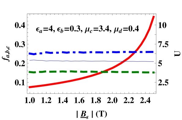
Figure 2: Implementation I. The common shape parameter $U$ (thick solid, red) and volume fractions $f_{a}$ (dashed, green), $f_{b}$ (broken dashed, blue), and $f_{c}$ (thin solid, blue) plotted versus $|{\underline{B}}_{\,s}|$ (T). The relative permittivities $\epsilon_{a}=4$, $\epsilon_{b}=0.3$, $\mu_{c}=3.4$ and $\mu_{d}=0.4$.

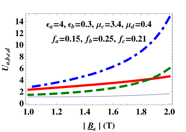
Figure 3: Implementation II. The shape parameters $U_{a}$ (thick solid, red), $U_{b}$ (dashed, green), $U_{c}$ (broken dashed, blue), and $U_{d}$ (thin solid, blue) plotted versus $|{\underline{B}}_{\,s}|$ (T). The relative permittivities $\epsilon_{a}=4$, $\epsilon_{b}=0.3$, $\mu_{c}=3.4$ and $\mu_{d}=0.4$; and the volume fractions $f_{a}=0.15$, $f_{b}=0.25$ and $f_{c}=0.21$.

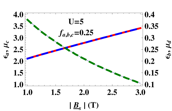
Figure 4: Implementation III. The relative permittivities $\epsilon_{a}$ (thick solid, red) and $\epsilon_{b}$ (dashed, green) and the relative permeabilities $\mu_{c}$ (broken dashed, blue) and $\mu_{d}$ (thin solid, blue) plotted versus $|{\underline{B}}_{\,s}|$ (T). The shape parameter $U=U_{a,b,c,d}=5$ and volume fractions $f_{a,b,c}=0.25$.

References

- [1] J. D. Jackson, Classical Electrodynamics, 3rd ed., Wiley, New York, NY, USA, 1999, pp. 9-13.
- [2] S. L. Adler, J. Phys. A: Math. Theor. 40 (2007) F143; correction: 40 (2007) 5767.
- [3] S. L. Adler, Ann. Phys. (NY) 67 (1971) 599.
- [4] E. Iacopini, E. Zavattini, Phys. Lett. B 85 (1979) 151.
- [5] E. Zavattini, G. Zavattini, G. Ruoso, E. Polacco, E. Milotti, M. Karuza, U. Gastaldi, G. Di Domenico, F. Della Valle, R. Cimino, S. Carusotto, G. Cantatore, M. Bregant, Phys. Rev. Lett. 96 (2006) 110406. See also Editorial Note, Phys. Rev. Lett. 99 (2007) 129901.
- [6] T. G. Mackay, A. Lakhtakia, Phys. Rev. B 83 (2011) 195424.
- [7] T. G. Mackay, A. Lakhtakia,
- [8] A. Lakhtakia, T. G. Mackay, Electromagnetics 27 (2007) 341.
- [9] W. Heisenberg, H. Euler, Z. Phys. 98 (1936) 714.
- [10] J. Schwinger, Phys. Rev. 82 (1951) 664.
- [11] M. Yan, W. Yan, M. Qiu, Prog. Opt. 52 (2009) 261.
- [12] W. S. Wiglhofer, A. Lakhtakia, B. Michel, Microw. Opt. Technol. Lett. 15 (1997) 263; correction: 22 (1999) 221.
- [13] T. G. Mackay, A. Lakhtakia, Electromagnetic Anisotropy and Bianisotropy: A Field Guide, World Scientific, Singaore, 2010, chap. 6.
- [14] A. Lakhtakia, Microw. Opt. Technol. Lett. 27 (2000) 175.
- [15] W. S. Weiglhofer, Microw. Opt. Technol. Lett. 28 (2001) 421.
- [16] E. Cherkaev, Inverse Problems 17 (2001) 1203.
- [17] T. G. Mackay, A. Lakhtakia, J. Nanophoton. 4 (2010) 041535.
- [18] S. S. Jamaian, T. G. Mackay, J. Nanophoton. 4 (2010) 043510.
- [19] T. G. Mackay, W. S. Weiglhofer, J. Opt. A: Pure Appl. Opt. 2 (2000) 426.
- [20] A. Alù, M. Silveirinha, A. Salandrino, N. Engheta, Phys. Rev. B 75 (2007) 155410.
- [21] G. Lovat, P. Burghignoli, F. Capolino, D. R. Jackson, IET Microw. Antennas Propagat. 1 (2007) 177.
- [22] M. N. Navarro-Cía, M. Beruete, I. Campillo, M Sorolla, Phys. Rev. B 83 (2011) 115112.