Edge Mode Combinations in the Entanglement Spectra of
Non-Abelian Fractional Quantum Hall States on the Torus

Abstract

We present a detailed analysis of bi-partite entanglement in the non-Abelian Moore-Read fractional quantum Hall state of bosons and fermions on the torus. In particular, we show that the entanglement spectra can be decomposed into intricate combinations of different sectors of the conformal field theory describing the edge physics, and that the edge level counting and tower structure can be microscopically understood by considering the vicinity of the thin-torus limit. We also find that the boundary entropy density of the Moore-Read state is markedly higher than in the Laughlin states investigated so far. Despite the torus geometry being somewhat more involved than in the sphere geometry, our analysis and insights may prove useful when adopting entanglement probes to other systems that are more easily studied with periodic boundary conditions, such as fractional Chern insulators and lattice problems in general.

I Introduction

Quantum correlations give rise to many exotic phases of matter that cannot be characterized in terms of traditional concepts, such as local order parameters and symmetry. Recently, tools from the field of quantum information (QI) have been used to quantify such correlations entrevs . Of special interest among the applications are systems in which more traditional condensed-matter methods are of limited use, for example topologically ordered matter toporder . Fractional quantum Hall (FQH) states stand out as experimentally verified topologically ordered phases driven by interactions, and their possible applications in the context of quantum computation are of great current interest topol-quantum-computing . The microscopic understanding of these phases is mainly based on ad hoc, albeit brilliant, guesswork laughlin83 ; mr ; jain89 ; greiter ; zhk ; nrft and numerical wave-function overlap calculations in small systems. A fundamental problem with using wave-function overlaps as a probe is, however, that it necessarily vanishes in the thermodynamic limit (for any realistic interaction). Recently, it has been realized that (bi-partite) entanglement measures, most saliently the von Neumann entropy kitaev06 ; levin06 and the entanglement spectrum LiH can provide valuable insights into these states—in principle even in the thermodynamic limit.

In this work, we focus our attention on entanglement in the archetypical non-Abelian FQH state, namely the Moore-Read state mr , which has received a tremendous amount of attention recently as a potential platform for topological quantum computation. Previous theoretical studiespfaffnum have accumulated evidence that the ground state of the two-dimensional electron gas at the Landau level filling fraction $\nu=5/2$ is well described by the Moore-Read state, which may be thought of as paired composite fermions and has quasiparticles possessing fractional charge $\pm e/4$ and obeying non-Abelian braid statistics mr . In recent experiments, both the fractional charge and non-Abelian braid statistics have been claimed MRexper , but the interpretations of the experiments is still under debatedebate . Another possible host of the Moore-Read state is the Bose-Einstein condensate under rapid rotation, in which the bosonic state at $\nu=1$ is particularly promising bosepfaff . However, the experimental realization of the bosonic FQHE is extremely challenging, although some strategies to overcome the difficulties have been proposedbec .

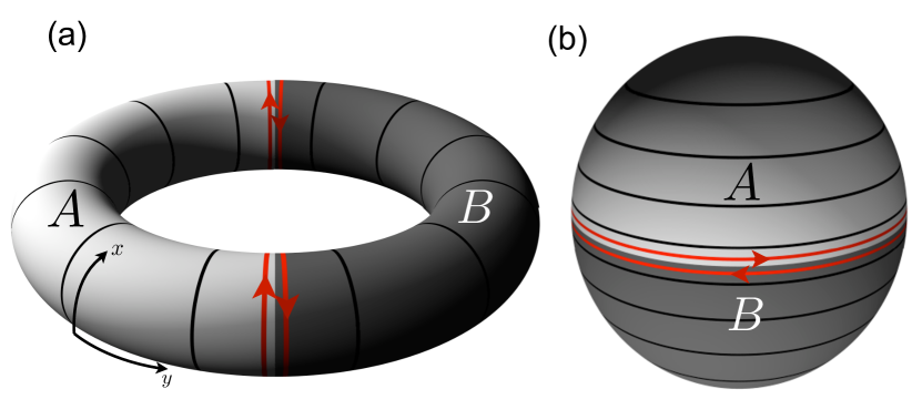
Figure 1: (Color online) The torus setup (a) compared with the orbital partition on the sphere (b). The dark lines indicate the centers of the single-particle states and the differently shaded regions denote the approximate spatial partitioning corresponding to the half-block orbital partitioning. Red arrows represent the artificial edge states induced by splitting the system into $A$ and $B$.

To study bi-partite entanglement, we (artificially) divide a system into two parts $A$ and $B$ (Fig. 1). In a tensor product Hilbert space, $\mathcal{H}=\mathcal{H}_{A}\otimes\mathcal{H}_{B}$, any pure state $|\Psi\rangle_{AB}$ can be decomposed using the Schmidt decompositionschmidt ,

$$|\Psi\rangle_{AB}=\sum_{i}e^{-\xi_{i}/2}|\psi_{i}^{A}\rangle\otimes|\psi_{i}^{B}\rangle,$$ (1)

where the states $|\psi_{i}^{A}\rangle$ ($|\psi_{i}^{B}\rangle$) form an orthonormal basis for the subsystem $A$ ($B$) and the entanglement “energies” $\xi_{i}\geq 0$ are related to the eigenvalues, $\lambda_{i}$, of the reduced density matrix, $\rho_{A}=\operatorname{tr}_{B}|\Psi\rangle_{AB\ AB}\langle\Psi|$, of $A$ as $\lambda_{i}=e^{-\xi_{i}}$.

For topologically ordered states in two dimensions, the entanglement entropy contains topological information about the state: $S_{A}=-\operatorname{tr}[\rho_{A}\ln\rho_{A}]=-\sum_{i}\lambda_{i}\ln\lambda_{i}=\sum_{i}\xi_{i}e^{-\xi_{i}}$, is expected to scale as

$$S_{A}\approx\alpha{L}-n\gamma+\mathcal{O}(1/L),$$

where $L$ is the (total) block boundary length, $n$ is the number of disconnected boundaries, and $\gamma$ characterizes the topological field theory describing the state kitaev06 ; levin06 .

Li and Haldane LiH realized that the full so-called entanglement spectrum (ES), $\{\xi_{i}\}$, contains much more information than entanglement entropy. In particular, when plotted against the natural quantum numbers of the system, it shows a remarkable similarity with the conformal field theory (CFT) describing the chiral edge states Wen_chiraledges of the FQH states.

To make practical use of the entanglement concepts, it is instrumental to find a protocol with which the theoretical ideas can be (numerically) tested in realistic circumstances. The most widely used concept of partitioning the system in terms of the single-particle orbitals was introduced by Haque, Zozulya, and Schoutens masud in their study of the topological entanglement entropy in Laughlin states on the sphere. A numerical determination of $\gamma$ (and $\alpha$) in realistic circumstances requires information about $S_{A}$ for a number of different boundary lengths, $L$. Because of its technical simplicity, early attempts to obtain the entropy scaling in FQH states focused on the sphere geometry masud . However, as recently demonstrated for Abelian FQH states, a substantially better finite size scaling can be obtained on the torus where the boundary length can be varied continuously by varying the aspect ratio gammatorus [cf. Fig. 1(a) and 1 (b)]. (The idea of obtaining entanglement entropy scaling through varying discrete torus circumferences was also used in Ref. triangulartorus, for the dimer model on the triangular lattice.) Importantly, this extra degree of freedom available on the torus also provides a handle on when the extrapolations needed to extract $\gamma$ can be trusted (and when they cannot).

With a few very recent exceptions chandran ; qi ; dubail , the efforts made in the study of the ES in FQH states are also numerical LiH ; ZozulyaHaqueRegnault ; RegnaultBernevigHaldane_PRL09 ; Lauchli ; ronny ; Zhao ; Schliemann ; zlatko ; antoine ; maria ; esdmrg ; peterson ; antoine2 . In addition to these works, there has been a large number of recent studies extending the range of applicability of the ES to an increasing number of physical systems moreES . The studies of the ES in FQH states have focused predominantly on the sphere geometry. In this case, there is a genuine benefit with this choice since it amounts to probing the physics of a single FQH edge while the natural partition on the torus corresponds to two oppositely oriented edges [cf. the red arrows in Fig. 1(a) and 1 (b), respectively]. A benefit with the torus setup is, however, that one can continuously connect to the exactly solvable thin-torus limit TT from which many of the properties of the ES can be understood microscopically Lauchli .

On the sphere one finds that the ES has a chiral structure LiH that is intimately related to the squeezing rule of model FQH states squeezing that holds on genus-0 manifolds. The structure of the squeezed configurations also provides physical insight similar to what is possible in the thin-torus limit. While the squeezing rule does not hold on the torus (genus-1), the ES can nevertheless be described by combining two edge spectra, as was shown in Ref. Lauchli, for the Laughlin state.

In spite of the technical difficulties involving two separate edges, these issues are worth dealing with, in particular since there are many physical systems of great interest that are only approachable using periodic boundary conditions. Specifically, regular two-dimensional lattices do not admit generally a defect-free embedding onto the sphere (because of their different Euler characteristics). In particular, the recently proposed fractional Chern insulatorsfchern ; chernins appear to belong to this category.

The two-edge picture on the torus is reportedlyantoine ; chernins difficult to extend to non-Abelian FQH states due to their non-trivial ground-state degeneracies, which do not result from simple center-of-mass translations as in the Abelian case. Thus, it is not a priori clear how to choose the ground state, $|\Psi\rangle_{AB}$, in (1) (or alternatively, how to define the density matrix of the full system $A\cup B$) out of this degenerate set. Note that the issue of degenerate ground states does not occur in the sphere case in which the model states are unique maximal density zero modes of their respective parent Hamiltonians.

Here, we adopt a very simple and natural choice for the set of $|\Psi\rangle_{AB}$ and show that a similar, but significantly richer, two-edge picture also holds true for the ES of non-Abelian FQH states on the torus. Specifically, we disentangle the physics of the edge modes appearing in the entanglement spectra in each of the topologically distinct sectors of the Moore-Read state of both fermions and bosons. We find that, even for a given cut in one of the ground states, the resulting towers are generated from combinations of different sectors of the underlying conformal field theory.

We also carefully analyze the scaling of the von Neumann entropy in the various sectors of the Moore-Read state. We find that the total entropy as well as the area-law entropy density, $\alpha$, can be estimated (in particular quite accurately in the case of bosons) while the extrapolation is too sensitive to faithfully determine the topological part, $\gamma$.

The remainder of this article is organized as follows. In Section II, we introduce the physical model and the method we use to obtain the ground states and calculate the ES. In Section III, we analyze the ES from two distinct perspectives. On the one hand, we explain the ES as the combination of edge modes and discuss the quantitative relation in this combination. On the other hand, we use the thin-torus limit and a perturbation theory to illuminate the microscopic origin of the observed ES, including the counting rules in different edge sectors. Finally, we discuss the entanglement entropy in Section IV.

II Model and method

We study a two-dimensional $N$-boson (fermion) system subject to a perpendicular magnetic field on a torus with periods $L_{1}$ and $L_{2}$ in the $x$ and $y$ directions. The full symmetry analysis of this system was first provided by Haldane haldane85 —here we use a convenient representation thereof. Periodic boundary conditions require that $L_{1}L_{2}=2\pi N_{s}$ (in units of the magnetic length) where $N_{s}$ is the (integer) number of magnetic flux quanta (the number of vortices for rotating Bose-Einstein condensates). We choose a basis of normalized single-particle lowest Landau level (LLL) wave functions as

$$\psi_{j}\!=\!\frac{1}{\sqrt{L_{1}\pi^{1/2}}}\sum_{n=-\infty}^{+\infty}e^{[\textrm{i}(\frac{2\pi j}{L_{1}}+nL_{2})x-(y+nL_{2}+\frac{2\pi j}{L_{1}})^{2}/2]},$$ (2)

where $j=0,1,2,...,N_{s}-1$ can be understood as the single-particle momentum in units of $2\pi/L_{1}$. Because $\psi_{j}$ is centered along the line $y=-2\pi j/L_{1}$, the whole system can be divided into $N_{s}$ orbitals that are spatially localized in the $y-$direction (but delocalized in the $x-$direction). There are two translation operators, $T_{\alpha}$, $\alpha=1,2$, that commute with the Hamiltonian $H$ (and any translational invariant operator); they obey $T_{1}T_{2}=e^{2\pi iN/N_{s}}T_{2}T_{1}$, and operators have eigenvalues $e^{2\pi iK_{\alpha}/N_{s}},K_{\alpha}=0,...,N_{s}-1$. $T_{1}$ corresponds to $x$-translations and $K_{1}=\sum_{i=1}^{N}j_{i}$ (mod $N_{s}$) is the total $x$-momentum in units of $2\pi/L_{1}$. $T_{2}$ translates a many-body state one lattice constant $L_{2}/N_{s}=2\pi/L_{1}$ in the $y$-direction and increases $K_{1}$ by $N$. At filling factor $\nu=p/q$ (with $p$ and $q$ co-prime), $T_{2}^{q}$ commutes with $T_{1}$, and $T_{2}^{k}$ ($k=0,1,\dots q-1$) generate $q$ degenerate orthogonal states, which have different $K_{1}$. This is the $q$-fold center of mass degeneracy common to all eigenstates of a translational invariant operator in a Landau level. Thus, the energy eigenstates are naturally labeled by a two-dimensional vector $K_{\alpha}=0,...,N_{s}/q-1$, where $e^{2\pi iK_{2}q/N_{s}}$ is the $T_{2}^{q}$-eigenvalue.

We use exact diagonalization to obtain the Moore-Read states, which are zero-energy ground states of certain three-body Hamiltonians (see Appendix A), in the orbital basis. The Moore-Read states are non-Abelian states, for which the degeneracy on the torus is enhanced (in this case by a factor $3$) compared to the $q$-fold degeneracy discussed above. It is readily seen from the thin-torus configurations (the ground states as $L_{1}\rightarrow 0$) that they are not simply the translations of each other TTpfaf (see below). To extract the ES, we choose the ground states as eigenstates of $T_{1}$ and $T_{2}^{q}$ and bipartition the system into blocks $A$ and $B$, which consist of $l_{A}$ consecutive orbitals and the remaining $N_{s}-l_{A}$ orbitals, respectively. We label every ES level by the particle number $N_{A}=\sum_{j\in A}n_{j}$ and the total momentum $K_{A}=\sum_{j\in A}jn_{j}$ (mod $N_{s}$) in block $A$, where $n_{j}$ is the particle number on the orbital $j$. (In this work, we present data only for the case in which $l_{A}=N_{s}/2$.)

To understand the ES, it is essential to understand what the partitioning of the state looks like in the thin-torus limit. For the bosonic case, there are three different thin-torus patterns leading to the following partitions (for $N=N_{s}=16$):

$$1111|\textbf{11111111}|1111$$ (3)

$$0202|\textbf{02020202}|0202\pm 2020|\textbf{20202020}|2020$$ .

For the fermionic case, there are six different thin torus patterns and the following partitions (for $N=16,N_{s}=32$):

$$01010101|\textbf{0101010101010101}|01010101$$ (4)

$$10101010|\textbf{1010101010101010}|10101010$$

$$01100110|\textbf{0110011001100110}|01100110\pm 10011001|\textbf{1001100110011001}|10011001$$

$$11001100|\textbf{1100110011001100}|11001100\pm 00110011|\textbf{0011001100110011}|00110011$$ .

The bold block is our subsystem $A$. For bosons in (3), we have two qualitatively different cuts: $11|\textbf{11}\cdots\textbf{11}|11$ and $02|\textbf{02}\cdots\textbf{02}|02$ ($20|\textbf{20}\cdots\textbf{20}|20$ gives a mirror image of this). For fermions in (4), we have four qualitatively different cuts: $01|\textbf{01}\cdots\textbf{01}|01$ ($10|\textbf{10}\cdots\textbf{10}|10$), $0110|\textbf{0110}\cdots\textbf{0110}|0110$, $1001|\textbf{1001}\cdots\textbf{1001}|1001$, and $1100|\textbf{1100}\cdots\textbf{1100}|1100$ ($0011|\textbf{0011}\cdots\textbf{0011}|0011$).

We stress that, as long as the edges are sufficiently well separated, one can understand the entanglement in terms of two non-interacting edges whose details depend on the local environment around the cuts Lauchli . This holds true also for the states that are connected to a thin-torus configuration which is a linear superposition of two individual terms—in these cases the ES is composed of two shifted and superimposed mirror images corresponding to the ES of a single term respectively.

Our procedure is different from that in Refs. antoine, ; chernins, where the authors calculate the ES via a mixed state density matrix of the form $\rho=\frac{1}{d}\sum_{i=1}^{d}|\Psi^{i}\rangle_{AB\ AB}\langle\Psi^{i}|$ where $\{|\Psi^{i}\rangle_{AB}\}$ denote $d$ degenerate ground states. With this recipe one finds that the ES corresponds to the superimposed ES of all the $d$ thin-torus patterns. For the entanglement entropy, such a mixed state prescription essentially shifts $S_{A}(L)$ by a constant and would thus result in a shifted prediction for the topological contribution, $\gamma$. In the case of Abelian states, it turns out that averaging the entropies (rather than the density matrices) over the different sectors, or equivalently over the possible translations of the region $A$, significantly reduces finite-size corrections and yields results in excellent agreement with theorygammatorus . We note that the mixed-state prescription shifts the entropies of Abelian states by a constant value, $\ln d$, and would thus lead to a topological entropy different from the theoretical predictions for the spatial (as opposed to orbital) cut—in fact, it would lead to $\gamma=0$. For non-Abelian states, it is not yet settled which orbital basis prescription would lead to the same topological entropy as for the spatial cut.

III Entanglement spectra: two-edge picture and thin-torus analysis

The most prominent $N_{A}$ sectors of the ES of the Moore-Read state for $N=16$ are displayed in Fig. 5 ($\nu=1$ bosons) and Fig. 6 ($\nu=1/2$ fermions). The gross features of the Moore-Read ES on the torus are very similar to that of the Laughlin state—in both cases, multiple towers are formedLauchli . In this section, we analyze the ES from two different perspectives: We explain the tower structure in terms of combinations of edge modes and highlight intriguing relations between the ES levels within the towers as well as between the levels in different particle number sectors. Moreover, we use the exactly solvable thin-torus limit and perturbation theory to understand the formation of various edge environments and towers.

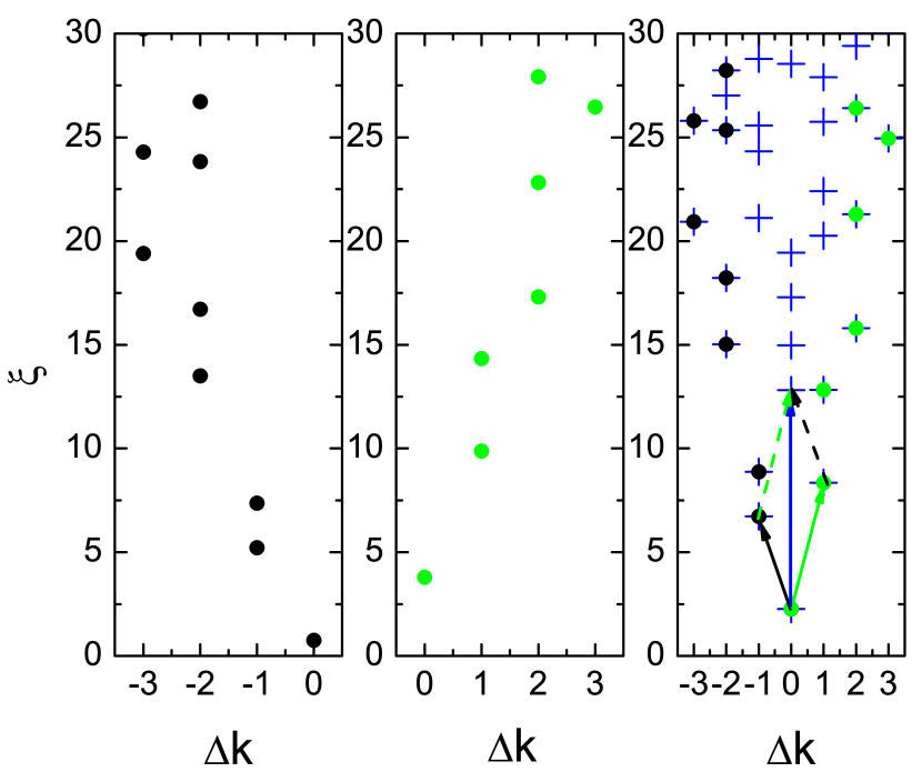
Figure 2: (color online) The edge modes of the environment in the left panel (black dots) and the environment in the middle panel (green dots) can combine to form a tower in the right panel (blue crosses). The relation in Eq. (5) is shown by the parallelogram. The edge mode at $\Delta k=-1$ pointed by the solid black arrow and the edge mode at $\Delta k=1$ pointed by the solid green arrow can generate the level at $\Delta k=0$ pointed by the solid blue arrow. This data comes from the ES of bosons in the 11 sector (see Fig. 5).

The observed towers in the numerical ES can be reproduced by first assigning the edge modes of individual edge environments and then combining them appropriately. The number of independent edge modes at momentum $\Delta k$ in an edge environment is determined by the underlying edge theory. The edge theory of the Moore-Read state is richer than that of the Laughlin state and contains a free boson branch as well as a Majorana fermion branchWen_pfcount . The details are recapitulated in Appendix B for completeness. It is important to note that there are different sectors of the edge theory and that they come with different predictions for the counting of states as a function of momentum. This is reflected in our numerically obtained ES, where we observe the edge environments with different counting rules. It is interesting to see that two edge environments with different counting rules can also combine to form a tower.

There are intriguing quantitative relations in the combination of edge modes as first pointed out for the Laughlin state in Ref. Lauchli, . An explicit example of how two edges, with different dispersion, add up to a tower is given in Fig. 2. More generally, each edge mode can be labeled by three parameters: the edge environment $\mathcal{X}$ to which it belongs, its momentum shift $\Delta k_{i}$ compared with the bottom mode of the environment $\mathcal{X}$, and the change of the subsystem particle number $\Delta N_{A}^{\mathcal{X}}$ in the environment $\mathcal{X}$ compared with the thin-torus state. Two edge modes with entanglement energy $\xi(\mathcal{X},\Delta k_{i},\Delta N_{A}^{\mathcal{X}})$ and $\xi(\mathcal{Y},\Delta k_{j},\Delta N_{A}^{\mathcal{Y}})$, respectively (here we assume $\Delta k_{i}\leq 0$ and $\Delta k_{j}\geq 0$), combine to form a level in the $\mathcal{X}\mathcal{Y}$ tower with entanglement energy

$$\xi(\mathcal{X}\mathcal{Y},\Delta k_{i}+\Delta k_{j},\Delta N_{A}^{\mathcal{X}}+\Delta N_{A}^{\mathcal{Y}})=\xi(\mathcal{X},\Delta k_{i},\Delta N_{A}^{\mathcal{X}})+\xi(\mathcal{Y},\Delta k_{j},\Delta N_{A}^{\mathcal{Y}})-\frac{1}{2}[\xi(\mathcal{X},0,\Delta N_{A}^{\mathcal{X}})+\xi(\mathcal{Y},0,\Delta N_{A}^{\mathcal{Y}})].$$ (5)

The validity of the two-edge picture is insensitive to the circumference $L_{1}$ as long as the edges are sufficiently well separated from each other, i.e. given that $d\sim L_{2}/2=\pi N_{s}/L_{1}$ is large enough, which is equivalent to small enough $L_{1}$ for a given system size. This is illustrated in Fig. 3, where the breakdown of the two-edge picture is signaled for the larger $L_{1}$ values, which is indeed a confirmation of the fact that the decomposition of the entire ES into a combination of edge modes is a highly non-trivial fact. Note that this breakdown occurs despite the fact that the numerically exact Moore-Read state is obtained for all $L_{1}$.

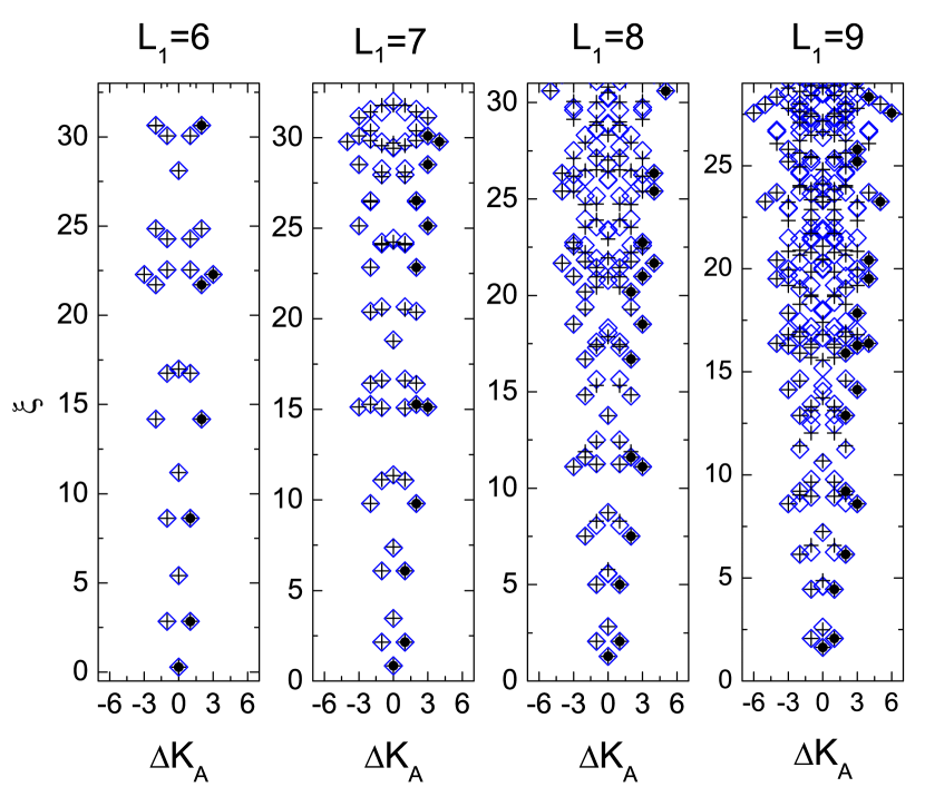
Figure 3: (color online) A plot of the main tower(s) of the ES in the 0101 fermionic Moore-Read state for various $L_{1}$ ($N_{A}=8,N=N_{s}/2=16$). For small enough $L_{1}$ (in this case $L_{1}\leq 7$ or so) the edges are well enough separated ($d\sim L_{2}/2=\pi N_{s}/L_{1}$) and the two-edge prediction (black crosses) reproduces the numerically obtained ES levels (blue squares). For larger $L_{1}$ the edges are spatially closer and the two-edge prediction gradually breaks down.

The relative pseudo-energies of the assigned single-edge modes depend smoothly on the torus thickness $L_{1}$, to some degree even after the two-edge prediction breaks down. For a given $L_{1}$, the edge levels correspond well to the single-edge levels extracted from the ES on a sphere with a corresponding length of the equator, as shown in Fig. 4. For large boundary lengths, the dispersion of a single edge becomes non-monotonic—at least in the case of fermions [cf Fig. 4(b)], as can be inferred from the original data obtained by Li and Haldane LiH . This does not imply that the two-edge picture will eventually break down, but does imply that the edge assignment becomes much more cumbersome at large $L_{1}$ as the $\Delta k=0$ levels no longer play the role of vacuum levels of each tower. Also, for this reason it is very useful to follow the evolution of the edge levels down to small $L_{1}$ where the dispersion is monotonic in order to eventually understand the ES also at large $L_{1}$ .

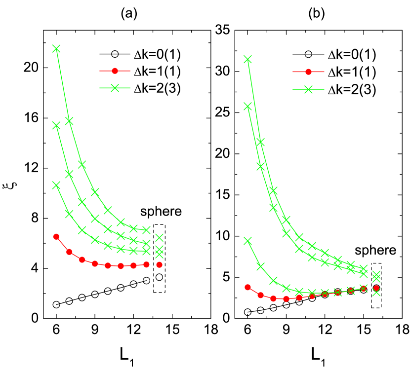
Figure 4: (color online) The single-edge modes identified from the ES as a function of $L_{1}$. (a) The edge modes corresponding to the $0|2$ cut in the bosonic Moore-Read state for $N=N_{s}=12$. (b) The edge modes corresponding to the $0|0$ cut in the fermionic Moore-Read state for $N=12$, $N_{s}=24$. The rectangles contain the single-edge ES levels in the spherical geometrynicolas , here shifted: $\{\xi_{i}\}\rightarrow\{\xi_{i}+{\rm constant}\}$, for the best comparison with the torus results at $L_{1}=14$ for bosons and $L_{1}=16$ for fermions. The number of flux quanta on the sphere $N_{s}^{\textrm{sp}}$ is chosen as the integer nearest to $L_{1}^{2}/(2\pi^{2})$ so that the length of the equator of the sphere is nearly the same with $L_{1}$. Here $N=12,N_{s}^{\textrm{sp}}=10$ for bosons and $N=8,N_{s}^{\textrm{sp}}=13$ for fermionsshift . One can see that in (b) the red dot is slightly lower than the black circle at $L_{1}=13$, meaning that a non-monotonic dispersion of the edge appears.

The adiabatic connection to the thin-torus ($L_{1}\rightarrow 0$) limit also enables us to understand more detailed features of the ES by perturbing away from this solvable limit Lauchli . The perturbation theory is however hard to perform in a rigorous way, as was recently performed for the ES of one-dimensional modelsAlba2011 . The reason for this is that the exponential behavior of the matrix elements implies that higher-order contributions from local terms come with amplitudes of the same order as longer-range terms contribute at lower orders. Nevertheless, many insights can be gained from a perturbative perspective, as we discuss below.

It is instructive to divide the perturbations, which are three-particle hopping processes, into three different classes. In the first class, three particles belong to the same subsystem and none of them move across the edge. These processes do not qualitatively alter the entanglement between two subsystems. In the second class, two particles belong to one subsystem and one particle belongs to the other, but still none of them moves across the edge. In the third class, some of the particles move across the edge. As we show below, the processes in the second class are responsible for generating new levels within a tower, and those in the third class lead to levels in new towers stemming from new edge environments. The entire ES of the Moore-Read state is built from successive combinations of many of the processes in each of these three classes.

With the knowledge of the microscopic environment near a cut in the thin-torus limit, the counting of each edge follows from the exclusion principle that no more than two bosons (fermions) occupy two (four) adjacent orbitals. Similar exclusion rules are, in addition to the thin-torus limitTTpfaf , also showing up in related approachesrelated ; squeezing such as the squeezing rules related to Jack polynomials and the patterns of zeros approach.

III.1 Bosons

We now give a more detailed account of the Moore-Read ES in the case of bosons.

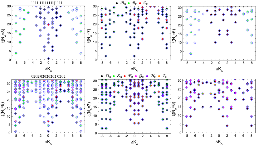
Figure 5: (color online) The ES of bosonic Moore-Read states in the 11 sector at $L_{1}=5.5$ (upper panels) and the 02+20 sector at $L_{1}=6$ (lower panels) for $N=N_{s}=16$. The origin of $\Delta K_{A}$ is chosen to match the Tao-Thouless state. The blue squares represent numerically obtained data. The assigned edge modes are labeled by dots with different colors corresponding to different edge environments we describe in the text. The combination of two identical edge environments is marked by the crosses with the color of that edge environment. The combination of two different edge environments is marked by the squares filled with two colors, the left (right) one of which corresponds to the edge environment on the left (right) edge of the subsystem $A$. Here we do not differentiate the edge environments $\mathcal{D}_{\textrm{B}}^{\prime}$ to $\mathcal{I}^{\prime}_{\textrm{B}}$ from the edge environments $\mathcal{D}_{\textrm{B}}$ to $\mathcal{I}_{\textrm{B}}$ because the former ones are just the mirror symmetries of the latter ones and have a momentum shift $\pm N_{s}/2$.

We first consider the 11 sector and systematically explain the ES in this sector, which is shown in Fig. 5. The lowest ES level is found in the $N_{A}=8$ sector at $\Delta K_{A}=0$, corresponding to the thin-torus configuration

$$1111|\textbf{11111111}|1111.$$

At $L_{1}=0$, this is the only entanglement level. We call the edge environment $1111|1111$ $\mathcal{A}_{\textrm{B}}$, where the subscript, B, indicates the environment is for bosons. Here the subsystem on the left (right) side of this edge environment is $A$ when we consider the right (left) edge of $A$. By definition $\Delta N_{A}^{\mathcal{A}_{\textrm{B}}}=0$. (In the following, when we discuss $\Delta N_{A}^{\mathcal{X}}$ of an edge environment $\mathcal{X}$, we suppose the subsystem $A$ is on the left side of $\mathcal{X}$. If $A$ is on the right side, one only needs to put a minus sign before the value that we give.) All other levels in the $\mathcal{A}_{\textrm{B}}\mathcal{A}_{\textrm{B}}$ tower ($\mathcal{A}_{\textrm{B}}\mathcal{A}_{\textrm{B}}$ denote the edge environments on the left and right edge of subsystem $A$) are generated from this level by the momentum-conserving hopping processes, which conserve $N_{A}$. For example, a hopping process at the right edge of subsystem $A$, $\textbf{1111}|1111\rightarrow\textbf{1102}|2011$, gives the lowest level at $\Delta K_{A}=1$.

Some processes do not conserve $N_{A}$; e.g., $1111|1111\rightarrow 1103|0111$ or $1111|1111\rightarrow 1110|3011$. We call the new kind of edge environment in this example $\mathcal{B}_{\textrm{B}}$. It is clear that $\Delta N_{A}^{\mathcal{B}_{\textrm{B}}}=\pm 1$. Two $\mathcal{B}_{\textrm{B}}$ edges create the $\mathcal{B}_{\textrm{B}}\mathcal{B}_{\textrm{B}}$ tower in the $N_{A}=8$ sector, whose dominant thin-torus configurations are:

$$1103|\textbf{01111103}|0111$$

$$1110|\textbf{30111110}|3011$$ .

Similarly, we can find another new edge environment. When applying a hopping process to the edge environment $\mathcal{B}_{\textrm{B}}$: $1103|0111\rightarrow 1005|0011$ or $1110|3011\rightarrow 1100|5001$, we obtain the edge environment $\mathcal{C}_{\textrm{B}}$ with $\Delta N_{A}^{\mathcal{C}_{\textrm{B}}}=\pm 2$. Two $\mathcal{C}_{\textrm{B}}$ edges create the $\mathcal{C}_{\textrm{B}}\mathcal{C}_{\textrm{B}}$ tower in the $N_{A}=8$ sector, whose thin-torus configurations are:

$$1005|\textbf{00111005}|0011$$

$$1100|\textbf{50011100}|5001$$ .

The different edges can combine with each other to form towers in other $N_{A}$ sectors. For example, in the $N_{A}=7$ sector we predict and observe $\mathcal{A}_{\textrm{B}}\mathcal{B}_{\textrm{B}}$, $\mathcal{B}_{\textrm{B}}\mathcal{A}_{\textrm{B}}$, $\mathcal{B}_{\textrm{B}}\mathcal{C}_{\textrm{B}}$ and $\mathcal{C}_{\textrm{B}}\mathcal{B}_{\textrm{B}}$ towers. In the $N_{A}=6$ sector, we can observe another $\mathcal{B}_{\textrm{B}}\mathcal{B}_{\textrm{B}}$ tower and $\mathcal{A}_{\textrm{B}}\mathcal{C}_{\textrm{B}}$ and $\mathcal{C}_{\textrm{B}}\mathcal{A}_{\textrm{B}}$ towers.

The $\mathcal{A}_{\textrm{B}}$, $\mathcal{B}_{\textrm{B}}$ and $\mathcal{C}_{\textrm{B}}$ edges are sufficient to accurately reproduce the ES of the $11$ sector up to $\xi=30$ for $L_{1}=5.5$, as shown in the upper panels of Fig. 5. For larger $L_{1}$ more towers appear and can be explained along the same lines.

Now we turn to the (asymmetric cut in the) 02+20 sector, for which the ES possesses more complicated structures than that in the 11 sector, as shown in Fig. 5. For simplicity, we start our analysis from only one term in the superposition of the thin-torus configuration, for example, from the term $0202|\textbf{02020202}|0202$. The entire ES in the 02+20 sector is recovered by superposing two mirror images of the ES stemming from the single term.

In the thin-torus limit, the only entanglement level at $\Delta K_{A}=0$ corresponds to the configuration

$$0202|\textbf{02020202}|0202.$$

We refer to this edge environment $0202|0202$ as $\mathcal{D}_{\textrm{B}}$. All other levels in the $\mathcal{D}_{\textrm{B}}\mathcal{D}_{\textrm{B}}$ tower are generated from this level by the momentum-conserving hopping processes, which conserve $N_{A}$.

Through applying leading hopping processes, we can generate all edge environments we have observed in the ES (at $L_{1}=6$):

$$\mathcal{D}_{\textrm{B}} :0202|0202,\Delta N_{A}^{\mathcal{D}_{\textrm{B}}}=0;$$

$$\mathcal{E}_{\textrm{B}} :0201|2102,\Delta N_{A}^{\mathcal{E}_{\textrm{B}}}=-1;$$

$$\mathcal{F}_{\textrm{B}} :0200|4002,\Delta N_{A}^{\mathcal{F}_{\textrm{B}}}=-2;$$

$$\mathcal{G}_{\textrm{B}} :0104|0102,\Delta N_{A}^{\mathcal{G}_{\textrm{B}}}=1;$$

$$\mathcal{H}_{\textrm{B}} :0006|0002,\Delta N_{A}^{\mathcal{H}_{\textrm{B}}}=2;$$

$$\mathcal{I}_{\textrm{B}} :0100|6001,\Delta N_{A}^{\mathcal{I}_{\textrm{B}}}=-3.$$

These edges combine with each other to form towers in each $N_{A}$ sector. For example, in the $N_{A}=8$ sector we predict and observe $\mathcal{D}_{\textrm{B}}\mathcal{D}_{\textrm{B}}$, $\mathcal{E}_{\textrm{B}}\mathcal{E}_{\textrm{B}}$, $\mathcal{F}_{\textrm{B}}\mathcal{F}_{\textrm{B}}$, $\mathcal{G}_{\textrm{B}}\mathcal{G}_{\textrm{B}}$ and $\mathcal{H}_{\textrm{B}}\mathcal{H}_{\textrm{B}}$ towers, Ii the $N_{A}=7$ sector we find $\mathcal{D}_{\textrm{B}}\mathcal{E}_{\textrm{B}}$, $\mathcal{E}_{\textrm{B}}\mathcal{F}_{\textrm{B}}$, $\mathcal{G}_{\textrm{B}}\mathcal{D}_{\textrm{B}}$, $\mathcal{H}_{\textrm{B}}\mathcal{G}_{\textrm{B}}$ and $\mathcal{F}_{\textrm{B}}\mathcal{I}_{\textrm{B}}$ towers, and in the $N_{A}=6$ sector we find $\mathcal{D}_{\textrm{B}}\mathcal{F}_{\textrm{B}}$, $\mathcal{G}_{\textrm{B}}\mathcal{E}_{\textrm{B}}$, $\mathcal{H}_{\textrm{B}}\mathcal{D}_{\textrm{B}}$ and $\mathcal{E}_{\textrm{B}}\mathcal{I}_{\textrm{B}}$ towers.

Similarly, we can start the analysis from the other term $2020|\textbf{20202020}|2020$ in the thin-torus configuration. We also predict and observe the six edge environments $\mathcal{D}^{\prime}_{\textrm{B}}$ to $\mathcal{I}^{\prime}_{\textrm{B}}$, which are just the mirror symmetries of the edge environments $\mathcal{D}_{\textrm{B}}$ to $\mathcal{I}_{\textrm{B}}$ for the term $0202|\textbf{02020202}|0202$. For example, the edge environment $\mathcal{D}^{\prime}_{\textrm{B}}$ is identified as $2020|2020$, which is the mirror symmetry of $\mathcal{D}_{\textrm{B}}$. Moreover, the combination of edge environments $\mathcal{D}^{\prime}_{\textrm{B}}$ to $\mathcal{I}^{\prime}_{\textrm{B}}$ can form towers in each $N_{A}$ sector. For example, in the $N_{A}=7$ sector we can observe the $\mathcal{E}^{\prime}_{\textrm{B}}\mathcal{D}^{\prime}_{\textrm{B}}$ tower as the mirror symmetry of the $\mathcal{D}_{\textrm{B}}\mathcal{E}_{\textrm{B}}$ tower.

We are also able to understand the counting rule of each edge environment from a simple exclusion rule in their thin-torus configuration. Here we take the edge environment $\mathcal{A}_{\textrm{B}}$ in the 11 sector and $\mathcal{D}_{\textrm{B}}$ in the 02+20 sector as examples. When analyzing the counting rule, we imagine the subsystem on the left (right) side of the edge environment as a quantum Hall system with an open right (left) edge, and then we move particles to the orbitals with higher (lower) momentum to increase (decrease) the momentum of the system. Meanwhile, the generalized exclusion ruleTTpfaf ; squeezing of the Moore-Read state, namely no more than two bosons (fermions) on two (four) consecutive orbits, should not be violated. Through the analysis, we can find that the counting rule of the edge environment $\mathcal{A}_{\textrm{B}}$ in the 11 sector is consistent with that of free bosons plus periodic Majorana fermions, while the counting rule of the edge environment $\mathcal{D}_{\textrm{B}}$ in the 02+20 sector is consistent with that of free bosons plus antiperiodic Majorana fermions with an even $F$ (see Appendix C). For some edge environments, only one side of it satisfies the generalized exclusion rule, for example the edge environment $\mathcal{E}_{\textrm{B}}=0201|2102$ in the 02+20 sector. In this case, we only need to analyze the subsystem on its left side. Through analysis, we can predict the counting rules of some edge environments and compare them with the counting rules that we observe in our numerical data. In the 11 sector, we have

$$\mathcal{A}_{\textrm{B}} :1,2,4,8,14,\cdots;[1,2,4,3];$$

$$\mathcal{B}_{\textrm{B}} :1,2,4,8,14,\cdots;[1,2,3,1];$$

$$\mathcal{C}_{\textrm{B}} :1,2,4,8,14,\cdots;[1,2,1]$$

and in the 02+20 sector, we have

$$\mathcal{D}_{\textrm{B}} :1,1,3,5,10,\cdots;[1,1,3,3,1];$$

$$\mathcal{E}_{\textrm{B}} :1,2,4,7,13,\cdots;[1,2,3,2,1];$$

$$\mathcal{F}_{\textrm{B}} :1,1,3,5,10,\cdots;[1,1,2,1];$$

$$\mathcal{G}_{\textrm{B}} :1,2,4,7,13,\cdots;[1,2,2];$$

$$\mathcal{H}_{\textrm{B}} :1,1,3,5,10,\cdots;[1,1];$$

$$\mathcal{I}_{\textrm{B}} :1,2,4,7,13,\cdots;[1],$$

where we, for each edge environment, first give the expected counting rule and then list the observed result from our numerical data, as shown in Fig. 5, in the brackets. For example, $\mathcal{A}_{\textrm{B}}:1,2,4,8,14,\cdots;[1,2,4,3]$ means that the expected number of edge modes for edge environment $\mathcal{A}_{\textrm{B}}$ is $1,2,4,8,14,\cdots$ at $\Delta k=0,1,2,3,4,\cdots$, while the observed number of edge modes is $1,2,4,3$ at $\Delta k=0,1,2,3$. We see that the numerically observed count never exceeds the theoretical expectations (that are derived for an infinite system). There are two reasons for this. First, our data are only numerically accurate up to some finite $\xi$, and thus we count only the levels that are free of numerical noise. Second, the counting is truncated by the finite system size similar to the situation on the sphere LiH ; maria and should be expected in any geometry.

III.2 Fermions

The thin-torus and edge analysis of the fermion ES (Fig. 6) is entirely analogous to the boson case, and thus we only provide a condensed exposition of the analysis here. Note however, that the edge assignment would have been much trickier in the fermion case if we would have started out by considering the large $L_{1}$ regime where the edge dispersion is non-monotonic LiH .

Figure 6: (color online) The ES of fermionic Moore-Read states in the 0101 sector at $L_{1}=7$ (upper panel), the 0110+1001 sector at $L_{1}=8$ (middle panel) and the 1100+0011 sector at $L_{1}=8$ (lower) for $N=16$, $N_{s}=32$. The origin of $\Delta K_{A}$ is chosen to match the thin-torus ground state. The blue squares represent numerically obtained data. The assigned edge modes are labeled by dots with different colors corresponding to different edge environments as described in the text. The combination of two identical edge environments is marked by the crosses with the color of that edge environment. The combination of two different edge environments is marked by the squares filled with two colors, the left (right) one of which corresponds to the edge environment on the left (right) edge of the subsystem $A$. Here we do not differentiate the edge environments $\mathcal{F}_{\textrm{F}}^{\prime}$ to $\mathcal{I}^{\prime}_{\textrm{F}}$ from $\mathcal{F}_{\textrm{F}}$ to $\mathcal{I}_{\textrm{F}}$ because the former ones are just the mirror symmetries of the latter ones and have a momentum shift $\pm N_{s}/2$.

In the 0101 sector, we can observe three edge environments:

$$\mathcal{A}_{\textrm{F}} :01010101|01010101,\Delta N_{A}^{\mathcal{A}_{\textrm{F}}}=0;$$

$$\mathcal{B}_{\textrm{F}} :01010100|11100101,\Delta N_{A}^{\mathcal{B}_{\textrm{F}}}=-1;$$

$$\mathcal{C}_{\textrm{F}} :00011111|00010101,\Delta N_{A}^{\mathcal{C}_{\textrm{F}}}=1.$$

Their counting rules are

$$\mathcal{A}_{\textrm{F}} :1,2,4,8,14,\cdots;[1,2,4,4,1];$$

$$\mathcal{B}_{\textrm{F}} :1,2,4,8,14,\cdots;[1,2,3,1];$$

$$\mathcal{C}_{\textrm{F}} :1,2,4,8,14,\cdots;[1,1],$$

which are the same as those for the 111 bosonic state. The combinations of edge environments can form towers in each $N_{A}$ sector: $\mathcal{A}_{\textrm{F}}\mathcal{A}_{\textrm{F}}$, $\mathcal{B}_{\textrm{F}}\mathcal{B}_{\textrm{F}}$ and $\mathcal{C}_{\textrm{F}}\mathcal{C}_{\textrm{F}}$ towers in the $N_{A}=8$ sector, $\mathcal{A}_{\textrm{F}}\mathcal{B}_{\textrm{F}}$ and $\mathcal{C}_{\textrm{F}}\mathcal{A}_{\textrm{F}}$ towers in the $N_{A}=7$ sector, and $\mathcal{C}_{\textrm{F}}\mathcal{B}_{\textrm{F}}$ tower in the $N_{A}=6$ sector.

In the 0110+1001 sector, first we start our analysis from the term $01100110|\textbf{0110011001100110}|01100110$. We find two edge environments:

$$\mathcal{D}_{\textrm{F}}: 01100110|01100110,\Delta N_{A}^{\mathcal{D}_{\textrm{F}}}=0;$$

$$\mathcal{E}_{\textrm{F}}: 01001111|00100110,\Delta N_{A}^{\mathcal{E}_{\textrm{F}}}=1;$$

$$01100100|11110010,\Delta N_{A}^{\mathcal{E}_{\textrm{F}}}=-1,$$

whose counting rules are expected as

$$\mathcal{D}_{\textrm{F}} :1,1,3,5,10,\cdots;[1,1,3,3,2,1];$$

$$\mathcal{E}_{\textrm{F}} :1,2,4,7,13,\cdots;[1,2,1].$$

If we start from the other term, $10011001|\textbf{1001100110011001}|10011001$, we also find the following two edge environments:

$$\mathcal{D}^{\prime}_{\textrm{F}}: 10011001|10011001,\Delta N_{A}^{\mathcal{D}^{\prime}_{\textrm{F}}}=0;$$

$$\mathcal{E}^{\prime}_{\textrm{F}}: 10011000|11110001,\Delta N_{A}^{\mathcal{E}^{\prime}_{\textrm{F}}}=-1;$$

$$10001111|00011001,\Delta N_{A}^{\mathcal{E}^{\prime}_{\textrm{F}}}=1,$$

with counting rules being

$$\mathcal{D}^{\prime}_{\textrm{F}} :1,2,4,7,13,\cdots;[1,2,4,3,1];$$

$$\mathcal{E}^{\prime}_{\textrm{F}} :1,1,3,5,10,\cdots;[1,1,2,1].$$

The combination of these edge environments can generate $\mathcal{D}_{\textrm{F}}\mathcal{D}_{\textrm{F}}$, $\mathcal{E}_{\textrm{F}}\mathcal{E}_{\textrm{F}}$, $\mathcal{D}^{\prime}_{\textrm{F}}\mathcal{D}^{\prime}_{\textrm{F}}$ and $\mathcal{E}^{\prime}_{\textrm{F}}\mathcal{E}^{\prime}_{\textrm{F}}$ towers in the $N_{A}=8$ sector; $\mathcal{D}_{\textrm{F}}\mathcal{E}_{\textrm{F}}$, $\mathcal{E}_{\textrm{F}}\mathcal{D}_{\textrm{F}}$, $\mathcal{D}^{\prime}_{\textrm{F}}\mathcal{E}^{\prime}_{\textrm{F}}$ and $\mathcal{E}^{\prime}_{\textrm{F}}\mathcal{D}^{\prime}_{\textrm{F}}$ towers in the $N_{A}=7$ sector; and $\mathcal{E}_{\textrm{F}}\mathcal{E}_{\textrm{F}}$ and $\mathcal{E}^{\prime}_{\textrm{F}}\mathcal{E}^{\prime}_{\textrm{F}}$ towers in the $N_{A}=6$ sector.

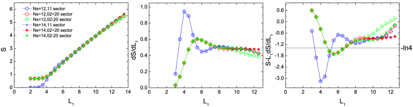
Figure 7: (color online) The bosonic Moore-Read state entropy $S_{A}$, its derivative $dS_{A}/dL_{1}$ and the intercept of its linear approximation $S_{A}-L_{1}\times dS_{A}/dL_{1}$ as functions of $L_{1}$ for $N=N_{s}=12$ and $N=N_{s}=14$ in the 11 sector, 02+20 sector and 02-20 sector. The theoretical value of the topological entropy $2\gamma=-\ln 4$ is indicated by the black line. In a rather large window of $L_{1}$, the entropy properties of the Moore-Read states in the 11 sector and 02+20 sector are quite similar.

In the 0011+1100 sector, if we start from the term $00110011|\textbf{0011001100110011}|00110011$, we find the following four edge environments:

$$\mathcal{F}_{\textrm{F}}: 00110011|00110011,\Delta N_{A}^{\mathcal{F}_{\textrm{F}}}=0;$$

$$\mathcal{G}_{\textrm{F}}: 00110010|11010011,\Delta N_{A}^{\mathcal{G}_{\textrm{F}}}=-1;$$

$$\mathcal{H}_{\textrm{F}}: 00110000|11111100,\Delta N_{A}^{\mathcal{H}_{\textrm{F}}}=-2;$$

$$\mathcal{I}_{\textrm{F}}: 00011111|00010011,\Delta N_{A}^{\mathcal{I}_{\textrm{F}}}=1,$$

with counting rules being

$$\mathcal{F}_{\textrm{F}} :1,1,3,5,10,\cdots;[1,1,3,3,1];$$

$$\mathcal{G}_{\textrm{F}} :1,2,4,7,13,\cdots;[1,2,3,2,1];$$

$$\mathcal{H}_{\textrm{F}} :1,1,3,5,10,\cdots;[1];$$

$$\mathcal{I}_{\textrm{F}} :1,2,4,7,13,\cdots;[1].$$

The combination of edges generates towers in each $N_{A}$ sector: $\mathcal{F}_{\textrm{F}}\mathcal{F}_{\textrm{F}}$ and $\mathcal{G}_{\textrm{F}}\mathcal{G}_{\textrm{F}}$ towers in the $N_{A}=8$ sector, $\mathcal{F}_{\textrm{F}}\mathcal{G}_{\textrm{F}}$, $\mathcal{G}_{\textrm{F}}\mathcal{H}_{\textrm{F}}$ and $\mathcal{I}_{\textrm{F}}\mathcal{F}_{\textrm{F}}$ towers in the $N_{A}=7$ sector, and $\mathcal{F}_{\textrm{F}}\mathcal{H}_{\textrm{F}}$ and $\mathcal{I}_{\textrm{F}}\mathcal{G}_{\textrm{F}}$ towers in the $N_{A}=6$ sector. If we start from the other term, $11001100|\textbf{1100110011001100}|11001100$, we find edge environments $\mathcal{F}^{\prime}_{\textrm{F}}$ to $\mathcal{I}^{\prime}_{\textrm{F}}$ which are just the mirror symmetries of $\mathcal{F}_{\textrm{F}}$ to $\mathcal{I}_{\textrm{F}}$ with the same counting rules. For example, the edge environment $\mathcal{F}^{\prime}_{\textrm{F}}$ is identified as $11001100|11001100$, which is the mirror symmetry of $\mathcal{F}_{\textrm{F}}$. Moreover, the combination of edge environments $\mathcal{F}^{\prime}_{\textrm{F}}$ to $\mathcal{I}^{\prime}_{\textrm{F}}$ forms towers in different $N_{A}$ sectors. For example, in the $N_{A}=7$ sector we predict and observe the $\mathcal{G}^{\prime}_{\textrm{F}}\mathcal{F}^{\prime}_{\textrm{F}}$ tower as the mirror symmetry of the $\mathcal{F}_{\textrm{F}}\mathcal{G}_{\textrm{F}}$ tower.

IV entanglement entropy

The entanglement entropy of the Moore-Read state was studied earlier on the sphere and disk geometry pfentropy , and the topological part, $\gamma$, has been reported to be consistent, albeit not in perfect agreement, with the theoretical predictions. However, the limitations of these geometrical setups make it very hard to verify whether the scaling regime (I) is reached or if the approximate agreement with theory is accidental. In addition, there are large finite size effects on the disk due to the (large) physical edge of the system. Here we revisit this issue using the torus setup that allows for superior control of the entanglement scaling properties as demonstrated for Abelian FQH states in Ref. gammatorus, . This method of partitioning implies two disjoint edges between the blocks, each of length $L_{1}$, so the entanglement entropy should satisfy the following specific scaling relation

$$S_{A}\approx 2\alpha L_{1}-2\gamma+\mathcal{O}(1/L_{1}),$$

where $\gamma$ is the topological entropy whose theoretical value is $\ln(\sqrt{4})$ for bosons and $\ln(\sqrt{8})$ for fermions kitaev06 ; levin06 . (See Ref. 2Dscaling, for the scaling relation of entanglement entropy in various physical systems.)

Figs. 7 and 8 show the entropy $S_{A}$, its derivative $dS_{A}/dL_{1}$, and the intercept of its linear approximation, $S_{A}-L_{1}\times dS_{A}/dL_{1}$, as functions of $L_{1}$ in different sectors for different system sizes. Arguably the boson results (Fig. 7) look more promising. In this case, the entropy in the different sectors differs for small $L_{1}$, as can be expected from the thin torus limit where the $20\pm 02$ states have an entropy of $\ln 2$ while the $11$ sector has zero entropy. However, from $L_{1}\approx 7$ the entropies, $S_{A}$, in the three sectors are very similar (left panel), although the more sensitive indicators $dS_{A}/dL_{1}$ (middle panel) and in particular $S_{A}-L_{1}\times dS_{A}/dL_{1}$ (right panel) show some differences. The density entropy in the bosonic More-Read state appears to be about $\alpha\approx 0.25$. In the case of fermions (Fig. 8), we find that the scaling regime is not yet reached, even though one may make a crude estimate of the entropy density, $\alpha\approx 0.2$.

The entropy density of a state is an indicator of how challenging it is to simulate the state on a classical computer, through a one-dimensional algorithm such as DMRG White ; dmrgrev , which has already been applied to the FQHE problem FQHDMRG , or through recently-proposed true two-dimensional algorithms like PEPS PEPS or MERA MERA . The larger entropy densities of Moore-Read states imply that they are more difficult to simulate than the Laughlin states.

Even for our largest system sizes, where we have obtained data for a range of $L_{1}$ values ($N=14$ for bosons and $N=16$ for fermions), we cannot extract a reliable topological entropy (see Figs. 7 and 8). However, we can observe some interesting phenomena. First, the entropy densities $\alpha=dS_{A}/d(2L_{1})$ of Moore-Read states are significantly larger than that of the fermionic Laughlin state at $\nu=1/3$ gammatorus and the bosonic Laughlin state at $\nu=1/2$ unpub . Second, the entropy properties of bosonic Moore-Read states in the 11 sector and those in the 02+20 sector become similar at large $L_{1}$. Their curves of $S_{A}$, $dS_{A}/dL_{1}$ and $S_{A}-L_{1}\times dS_{A}/dL_{1}$ overlap after $L_{1}\thickapprox 10$.

Let us also highlight some of the finite size features. For small $L_{1}$ the finite size convergence is essentially perfect and the curves for different system sizes are on top of each other in a given sector. At larger $L_{1}$, the curves show a stronger dependence on $N_{s}$. The $N_{s}$-dependence shows up first for the smallest system size and at increasing $L_{1}$ for progressively larger system sizes. This reflects the fact that, for any finite-size system, at very large $L_{1}$ the edges of block $A$ get too close and cannot be thought of as independent. In particular, once $L_{1}$ exceeds some value, we enter the thick-torus limit, and the entanglement entropy goes to some ($N$ dependent) saturation value. Corresponding to the saturation of $S_{A}$, the derivative $dS_{A}/dL_{1}$ drops to zero after some $L_{1}$. Therefore, the appropriate scaling regime of the entropy, $S_{A}$, may be expected to be valid only in a window of $L_{1}$, after the $\mathcal{O}(1/L_{1})$ term is small enough but before $S_{A}$ saturates. This analysis was shown to provide excellent results for abelian FQH states in Ref. gammatorus, . However, as already mentioned, we find that the finite size corrections to the scaling are too large to faithfully determine the topological part, $\gamma$, of the entropy for the Moore-Read state. Given the limitations encountered also in other geometries, we conclude that an accurate and reliable determination $\gamma$ for the Moore-Read state remains a challenge for the future.

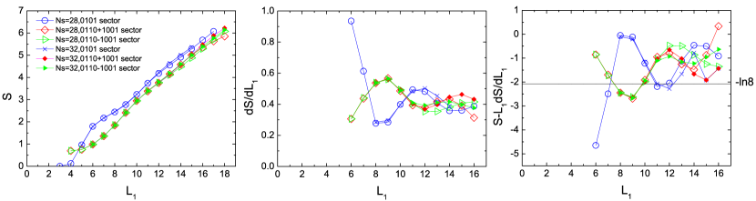
Figure 8: (color online) The fermionic Moore-Read state entropy $S_{A}$, its derivative $dS_{A}/dL_{1}$ and the intercept of its linear approximation $S_{A}-L_{1}\times dS_{A}/dL_{1}$ as functions of $L_{1}$ for $N_{s}=28$ and $N_{s}=32$ in the 0101 sector, 0110+1001 sector and 0110-1001 sector. The theoretical value of the topological entropy $2\gamma=-\ln 8$ is indicated by the black line. For the cut in the $0011\pm 1100$ sector is equivalent to a translation of the cut in the $0110\pm 1001$ sector. Therefore we make an average over their entropies and only show the averaged results (referred to as the $0110\pm 1001$ sector in above).

V Discussion

We have investigated the entanglement spectrum (ES) and the von Neumann entropy of bosonic and fermionic Moore-Read states on the torus. The ES on the torus is much more intricate and the analysis thereof poses a number of challenges compared to the sphere geometry where there is a single edge and a unique ground state. One such challenge is that in a given particle number sector, several towers appear due to possible compensating charge transfer across the two boundaries.

The study of the entanglement in this geometry is nevertheless well motivated as it provides new insights, for instance by connecting to the vicinity of the microscopically well understood thin-torus limit, and also because it may provide guidance for future studies of entanglement in other many-body systems where no natural analog to the quantum Hall sphere exists. In particular, the recently suggested fractional Chern insulators fchern ; chernins are most naturally studied using periodic boundary conditions, i.e. on a torus.

In this work we have suggested a procedure in order to resolve the problem of the non-trivial ground-state degeneracy on the torus: we used exact diagonalization and choose to calculate the entanglement in the pure (simultaneous) eigenstates of $H$, $T_{1}$ and $T_{2}^{q}$. This is different from the mixed-state recipe of Refs. antoine, ; chernins, , for which we expect a superimposed entanglement spectrum and a shifted prediction of the topological entropy $\gamma$.

For the ES, we found a tower structure similar to, but significantly richer than, what was found earlier in the ES of the Laughlin state. We used two complementary ideas in order to disentangle the ES by extending the results of Ref. Lauchli, to non-Abelian states. The first approach is based on a combination of two chiral CFT edges. Each of these is individually similar to the edge spectrum previously extracted from ES studies on the sphere. This interpretation is powerful as it reproduces the entire ES through the assignment of a few levels. It also reflects the intricate structure of the correlations in the Moore-Read state: Even for one cut of our system, edges corresponding to different topological sectors with different counting rules combine to form towers. Our second approach uses the adiabatic connection to the thin-torus limit: A perturbation analysis away from the thin-torus states yields the locations of the towers, and the counting rule of each edge environment follows from a generalized exclusion principle in the occupation number basis.

A further difficulty encountered when disentangeling the torus ES is the non-monotonic dispersion that appears for fermions at large $L_{1}$, as the lack of a natural vacuum level at the bottom/center of each tower severely increases the difficulty of the assignment of the edge modes. In the present case, this difficulty can be circumvented by following the smooth dependence of the edge levels to the small $L_{1}$ regime, where the dispersion is always monotonic.

For the von Neumann entropy, we found that the area-law entropy density, $\alpha=dS_{A}/dL_{1}\approx 0.20-0.25$ (per magnetic length), is larger than in the Laughlin states for both bosons and fermions. However, the comparable smallness of $\alpha$ is nevertheless encouraging regarding the possibilities of simulating the Moore-Read state using entanglement-based algorithms. Our results also show that an accurate and reliable determination $\gamma$ for the Moore-Read state on the torus remains a challenge for the future. It is likely that alternative methods, such as DMRG in a cylinder setup, will be needed to reach this goal.

The generalization of the analysis given here for the Moore-Read state to more generic non-abelian FQH states should be straight forward, but nevertheless interesting. The generalization to fractional Chern insulators is more challenging, but is likely to be rewarding.

Appendix A Hamiltonian generating Moore-Read states

The bosonic and fermionic Moore-Read states on the torus are the unique zero-energy ground states of translational invariant three-body interaction Hamiltonians

$$H=\sum_{\{k\}}\delta^{\prime}_{k_{1}+k_{2}+k_{3},k_{4}+k_{5}+k_{6}}V_{\{k\}}a_{k_{1}}^{\dagger}a_{k_{2}}^{\dagger}a_{k_{3}}^{\dagger}a_{k_{4}}a_{k_{5}}a_{k_{6}},$$

(6)

where $\{k\}=k_{1},k_{2},k_{3},k_{4},k_{5},k_{6}$, $a_{k}$ ($a_{k}^{\dagger}$) annihilates (creates) a boson or a fermion in the state $\psi_{k}$ in Eq. (2),

$$V_{\{k\}} = \sum_{\{s\},\{t\}=-\infty}^{+\infty}\delta^{\prime}_{s_{1},k_{1}-k_{6}}\delta^{\prime}_{s_{2},k_{2}-k_{5}}P(\{s\},\{t\})$$

$$\times \exp\Big{\{}-\frac{2\pi^{2}}{L_{1}^{2}}(s_{1}^{2}+s_{2}^{2}+s_{1}s_{2})-\frac{2\pi^{2}}{L_{2}^{2}}(t_{1}^{2}+t_{2}^{2}+t_{1}t_{2})\Big{\}}$$

$$\times \exp\Big{\{}\frac{\textrm{i}\pi}{N_{s}}t_{1}(2k_{3}-2k_{1}+2s_{1}+s_{2})\Big{\}}$$

$$\times \exp\Big{\{}\frac{\textrm{i}\pi}{N_{s}}t_{2}(2k_{3}-2k_{2}+s_{1}+2s_{2})\Big{\}},$$

and $\delta^{\prime}$ is the periodic Kronecker delta function with period $N_{s}$. $P(\{s\},\{t\})$ is a certain polynomial of $s_{1},s_{2},t_{1},t_{2}$, exact form of which depends on the targeted filling fraction.

We use exact diagonalization to obtain the ground states of (6) after choosing a proper form of $P$. Up to a constant factor, when $P=1$, (6) can generate the bosonic Moore-Read states at filling factor $\nu=1$, while when $P=-(4\pi^{2})^{3}(s_{1}^{2}/L_{1}^{2}+t_{1}^{2}/L_{2}^{2})[(s_{1}-s_{2})^{2}/L_{1}^{2}+(t_{1}-t_{2})^{2}/L_{2}^{2}]$, (6) can generate the fermionic Moore-Read states at filling factor $\nu=1/2$.

Table 1: In this table, we analyze the counting rule of the edge environment $\mathcal{A}_{\textrm{B}}$ in the 11 sector, which is $1,2,4,8,14,\cdots$ at $\Delta k=0,1,2,3,4,\cdots$.

$\Delta k=0$	$\Delta k=1$	$\Delta k=2$	$\Delta k=3$	$\Delta k=4$
$1111111111|0000$	$1111111110|1000$	$1111111110|0100$	$1111111110|0010$	$1111111110|0001$
	$1111111102|0000$	$1111111101|1000$	$1111111101|0100$	$1111111101|0010$
		$1111110202|0000$	$1111110201|1000$	$1111110201|0100$
		$1111111020|1000$	$1111111020|0100$	$1111111020|0010$
			$1111111100|2000$	$1111111100|1100$
			$1111020202|0000$	$1111020201|1000$
			$1111102020|1000$	$1111102020|0100$
			$1111111011|1000$	$1111111011|0100$
				$1111110200|2000$
				$1111110111|1000$
				$1111111010|2000$
				$1102020202|0000$
				$1111102011|1000$
				$1110202020|1000$

Table 2: In this table, we analyze the counting rule of the edge environment $\mathcal{D}_{\textrm{B}}$ in the 02+20 sector, which is $1,1,3,5,10,\cdots$ at $\Delta k=0,1,2,3,4,\cdots$.

$\Delta k=0$	$\Delta k=1$	$\Delta k=2$	$\Delta k=3$	$\Delta k=4$
$0202020202|0000$	$0202020201|1000$	$0202020201|0100$	$0202020201|0010$	$0202020201|0001$
		$0202020200|2000$	$0202020200|1100$	$0202020200|1010$
		$0202020111|1000$	$0202020111|0100$	$0202020111|0010$
			$0202020110|2000$	$0202020110|1100$
			$0202011111|1000$	$0202011111|0100$
				$0202020200|0200$
				$0202020102|0100$
				$0202020020|2000$
				$0202011110|2000$
				$0201111111|1000$

Appendix B Edge excitation of Moore-Read state

Compared with the Laughlin state, the edge excitations of the Moore-Read state are richer. It has one branch of free bosons and one branch of Majorana fermions obeying either antiperiodic (7) or periodic boundary conditions (8).

For free bosons plus antiperiodic Majorana fermions, the excitation spectrum is described by the Hamiltonian

$$H_{\textrm{edge}}^{\textrm{AP}}=\sum_{m>0}[E_{b}(m)b_{m}^{\dagger}b_{m}+E_{f}(m-1/2)c_{m-1/2}^{\dagger}c_{m-1/2}],$$ (7)

where $b$ and $b^{\dagger}$ ($c$ and $c^{\dagger}$) are standard boson (fermion) creation and annihilation operators, $E_{b}(m)$ [$E_{f}(m)$] is the dispersion relation of bosons (fermions) and the total momentum operator is defined as $K=\sum_{m>0}[mb_{m}^{\dagger}b_{m}+(m-1/2)c_{m-1/2}^{\dagger}c_{m-1/2}]$. The counting rule of the edge excitations, namely the number of energy levels at each $K$, depends on the parity of the number of fermions $(-1)^{F},F=\sum_{m>0}c_{m-1/2}^{\dagger}c_{m-1/2}$. For even $F$, the counting rule is $1,1,3,5,10,\cdots$ at $\Delta k=0,1,2,3,4,\cdots$; while for odd $F$, the counting rule is $1,2,4,7,13,\cdots$ at $\Delta k=0,1,2,3,4,\cdots$. Here $\Delta k$ is defined as $K-K_{0}$ where $K_{0}$ is the lowest momentum ($K_{0}=0$ for even $F$ and $K_{0}=1/2$ for odd $F$).

For free bosons plus periodic Majorana fermions, the edge excitation Hamiltonian is

$$H_{\textrm{edge}}^{\textrm{P}}=\sum_{m>0}[E_{b}(m)b_{m}^{\dagger}b_{m}+E_{f}(m-1)c_{m-1}^{\dagger}c_{m-1}],$$ (8)

for which the total momentum is $K=\sum_{m>0}[mb_{m}^{\dagger}b_{m}+(m-1)c_{m-1}^{\dagger}c_{m-1}]$. Through a similar analysis with that for the antiperiodic case, one can get that the counting rule is $1,2,4,8,14,\cdots$ at $\Delta k=0,1,2,3,4,\cdots$ for both even and odd $F=\sum_{m>0}c_{m-1}^{\dagger}c_{m-1}$.

The counting of each edge environment observed in our ES should be consistent with one of the four sectors here before the finite size effect truncates the series after some $\Delta k$ depending on the system size.

Appendix C The counting rules of edge environments

Here we analyze the counting rules of the edge environment $\mathcal{A}_{\textrm{B}}$ in the 11 sector and the edge environment $\mathcal{D}_{\textrm{B}}$ in the 02+20 sector. The results are obtained by applying the generalized exclusion rule on their thin-torus limit. All possible edge excitations at each $\Delta k$ are listed in Tables 1 and 2.

References

- (1) L. Amico, R. Fazio, A. Osterloh, and V. Vedral, Rev. Mod. Phys. 80, 517 (2008); J. Eisert, M. Cramer, M.B. Plenio, Rev. Mod. Phys. 82, 277 (2010).
- (2) See e.g. X.-G. Wen, Quantum Field Theory of Many-body Systems, (Oxford University Press, Oxford, 2004).
- (3) M. Freedman, M. Larsen, and Z. Wang, Commun. Math. Phys. 227, 605 (2002). S. Das Sarma, M. Freedman, and C. Nayak, Physics Today, 59, 32 (2006). C. Nayak, S. H. Simon, A. Stern, M. Freedman, and S. Das Sarma, Rev. Mod. Phys. 80, 1083 (2008).
- (4) R. B. Laughlin, Phys. Rev. Lett. 50, 1395 (1983).
- (5) G. Moore, and N. Read, Nucl. Phys. B 360, 362 (1991).
- (6) J. K. Jain, Phys. Rev. Lett. 63, 199 (1989).
- (7) M. Greiter, X.G. Wen, and F. Wilczek, Phys. Rev. Lett 66, 3205 (1991); Nucl. Phys. B 374, 567 (1992).
- (8) S. C. Zhang, T. H. Hansson and S. Kivelson, Phys. Rev. Lett. 62, 82 (1989).
- (9) N. Read, Phys. Rev. Lett. 62, 86 (1989).
- (10) A. Kitaev and J. Preskill, Phys. Rev. Lett. 96, 110404-1 (2006).
- (11) M. Levin and X. G. Wen, Phys. Rev. Lett. 96, 110405 (2006).
- (12) H. Li and F. D. M. Haldane, Phys. Rev. Lett. 101, 010504 (2008).
- (13) R.H. Morf, Phys. Rev. Lett. 80, 1505 (1998); E.H. Rezayi, and F.D.M. Haldane, Phys. Rev. Lett. 84, 4685 (2000).
- (14) See e.g. M. Dolev, M. Heiblum, V. Umansky, A. Stern and D. Mahalu, Nature 452, 829 (2008); I. P. Radu, J. B. Miller, C. M. Marcus, M. A. Kastner, L. N. Pfeiffer and K. W. West, Science, 320, 899 (2008); R. L. Willett, L. N. Pfeiffer, and K. W. West, Phys. Rev. B 82, 205301 (2010).
- (15) K. Shtengel, Physics 3, 93 (2010).
- (16) N.K. Wilkin, and J.M.F. Gunn, Phys. Rev. Lett. 84, 6 (2000); N. Regnault, and Th. Jolicoeur, Phys. Rev. Lett. 91, 030402 (2003); E. Wikberg, E. J. Bergholtz and A. Karlhede, J. Stat. Mech. (2009) P07038.
- (17) I. Bloch, J. Dalibard, and W. Zwerger, Rev. Mod. Phys. 80, 885 (2008); A. L. Fetter, Rev. Mod. Phys. 81, 647 (2009). M. Roncaglia, M. Rizzi and J. Dalibard, Scientific Reports 1, 43 (2011) .
- (18) See e.g. M. A. Nielsen and I. L. Chuang: Quantum Computation and Quantum information, Cambridge University Press, Cambridge 2000.
- (19) X. G. Wen, Phys. Rev. B 41, 12838 (1990).
- (20) M. Haque, O. Zozulya and K. Schoutens, Phys. Rev. Lett. 98, 060401 (2007).
- (21) A.M. Läuchli, E. J. Bergholtz and M. Haque, New J. Phys. 12, 075004 (2010).
- (22) S. Furukawa and G. Misguich, Phys. Rev. B 75, 214407 (2007).
- (23) A. Chandran, M. Hermanns, N. Regnault, and B.A. Bernevig, Phys. Rev. B 84, 205136 (2011).
- (24) X.-L. Qi, H. Katsura, and A. W. W. Ludwig, arXiv:1103.5437.
- (25) J. Dubail and N. Read, Phys. Rev. Lett. 107, 157001 (2011).
- (26) O. S. Zozulya, M. Haque and N. Regnault, Phys. Rev. B 79, 045409 (2009).
- (27) N. Regnault, B. A. Bernevig, and F. D. M. Haldane, Phys. Rev. Lett. 103, 016801 (2009).
- (28) A. M. Läuchli, E. J. Bergholtz, J. Suorsa, and M. Haque, Phys. Rev. Lett., 104, 156404 (2010).
- (29) R. Thomale, A. Sterdyniak, N. Regnault, and B. A. Bernevig, Phys. Rev. Lett. 104, 180502 (2010).
- (30) Z. Liu, H.-L. Guo, V. Vedral, and H. Fan Phys. Rev. A 83, 013620 (2011).
- (31) J. Schliemann, Phys. Rev. B 83, 115322 (2011).
- (32) Z. Papic, B. A. Bernevig, and N. Regnault, Phys. Rev. Lett. 106, 056801 (2011).
- (33) A. Sterdyniak, N. Regnault, and B. A. Bernevig, Phys. Rev. Lett. 106, 100405 (2011).
- (34) M. Hermanns, A. Chandran, N. Regnault, and B. Andrei Bernevig, Phys. Rev. B 84, 121309(R) (2011) .
- (35) J. Zhao, D. N. Sheng, and F. D. M. Haldane, Phys. Rev. B 83, 195135 (2011).
- (36) J. Biddle, Michael R. Peterson, and S. Das Sarma, Phys. Rev. B 84, 125141 (2011) .
- (37) A. Sterdyniak, B.A. Bernevig, N. Regnault, and F. D. M. Haldane, New J. Phys. 13, 105001 (2011).
- (38) P. Calabrese and A. Lefevre, Phys. Rev. A 78, 032329 (2008); F. Pollmann, A. M. Turner, E. Berg, M. Oshikawa, Phys. Rev. B 81, 064439 (2010); D. Poilblanc, Phys. Rev. Lett. 105, 077202 (2010); I. Peschel and M.-C. Chung, Europhys. Lett. 96, 50006 (2011); H. Yao and X.-L. Qi, Phys. Rev. Lett. 105, 080501 (2010); E.J. Bergholtz, M. Nakamura and J. Suorsa, Physica E 43, 755 (2011); J. I. Cirac, D. Poilblanc, N. Schuch, and F. Verstraete, Phys. Rev. B 83, 245134 (2011); C.-Y. Huang and F. L. Lin, Phys. Rev. B 84, 125110 (2011); L. Fidkowski, Phys. Rev. Lett. 104, 130502 (2010); E. Prodan, T. L. Hughes, and B. A. Bernevig, Phys. Rev. Lett 105, 115501 (2010); S. Furukawa and Y.-B. Kim, Phys. Rev. B 83, 085112 (2011); X. Deng and L. Santos, Phys. Rev. B 84, 085138 (2011); A. M. Läuchli and J. Schliemann, arXiv:1106.3419; A. M. Turner, F. Pollmann, and E. Berg, Phys. Rev. B 83, 075102 (2011); J. Lou, S. Tanaka, H. Katsura, N. Kawashima, Phys. Rev. B 84, 245128 (2011).
- (39) E. J. Bergholtz and A. Karlhede, Phys. Rev. Lett. 94, 026802 (2005); J. Stat. Mech. L04001 (2006); Phys. Rev. B 77, 155308 (2008); A. Seidel, H. Fu, D.-H. Lee, J. M. Leinaas, and J. Moore, Phys. Rev. Lett. 95, 266405 (2005).
- (40) B.A. Bernevig, and F.D.M. Haldane, Phys. Rev. Lett. 100, 246802 (2008); M. Greiter, Bull. Am. Phys. Soc. 38, 137 (1993).
- (41) E. Tang, J.-W. Mei, and X.-G. Wen, Phys. Rev. Lett. 106, 236802 (2011); T. Neupert, L. Santos, C. Chamon, and C. Mudry, Phys. Rev. Lett. 106, 236804 (2011); K. Sun, Z. Gu, H. Katsura, and S. Das Sarma, Phys. Rev. Lett. 106, 236803 (2011).
- (42) N. Regnault, B. Andrei Bernevig, Phys. Rev. X 1, 021014 (2011).
- (43) F.D.M. Haldane, Phys. Rev. Lett. 55, 2095 (1985).
- (44) E.J. Bergholtz, J. Kailasvuori, E. Wikberg, T.H. Hansson, and A. Karlhede, Phys. Rev. B 74, 081308(R) (2006); A. Seidel, and D.-H. Lee, Phys. Rev. Lett. 97, 056804 (2006); E. Ardonne, E. J. Bergholtz, J. Kailasvuori, and E. Wikberg, J. Stat. Mech. (2008) P04016.
- (45) X.-G. Wen, Phys. Rev. Lett. 70, 355 (1993); M. Milovanovic and N. Read, Phys. Rev. B 53, 13559 (1996).
- (46) V. Alba, M. Haque, and A. M. Läuchli, arXiv:1107.1726;
- (47) N. Regnault, unpublished.
- (48) For the clustered (Read-Rezayi) quantum Hall states at on the sphere, one can derive . Therefore, for bosonic Moore-Read state ( and ), and for fermionic Moore-Read state ( and ), .
- (49) X.-G. Wen and Z. Wang, Phys. Rev. B 78, 155109 (2008); M. Barkeshli and X.-G. Wen, Phys. Rev. B 79, 195132 (2009); B.A. Bernevig and F.D.M. Haldane, Phys. Rev. Lett. 102, 066802 (2009); R. Thomale, B. Estienne, N. Regnault and B. A. Bernevig, Phys. Rev. B 84, 045127 (2011); M. Kardell and A. Karlhede J. Stat. Mech. P02037 (2011).
- (50) O. S. Zozulya, M. Haque, K. Schoutens, and E. H. Rezayi, Phys. Rev. B 76, 125310 (2007); A. G. Morris and D. L. Feder, Phys. Rev. A 79, 013619 (2009).
- (51) D. Gioev and I. Klich, Phys. Rev. Lett. 96, 100503 (2006); M. M. Wolf, Phys. Rev. Lett. 96, 010404 (2006); E. Fradkin and J. E. Moore, Phys. Rev. Lett. 97, 050404 (2006); T. Barthel, M. C. Chung and U. Schollwöck, Phys. Rev. A 74, 022329 (2006); W. Li, L. Ding, R. Yu, T. Roscilde, and S. Haas, Phys. Rev. B 74, 073103 (2006); L. Ding, N. Bray-Ali, R. Yu, and S. Haas, Phys. Rev. Lett. 100, 215701 (2008); R. Yu, H. Saleur, and S. Haas, Phys. Rev. B 77, 140402(R) (2008); B. Hsu, M. Mulligan, E. Fradkin, and E.A. Kim, Phys. Rev. B 79, 115421 (2009); I. D. Rodriguez and G. Sierra, Phys. Rev. B 80, 153303 (2009); N. Bray-Ali, L. Ding, and S. Haas, Phys. Rev. B 80, 180504 (2009); L. Tagliacozzo, G. Evenbly, and G. Vidal, Phys. Rev. B 80, 235127 (2009); S. V. Isakov, M. B. Hastings, R. G. Melko, Nature Phys. 7, 772 (2011). ; Y. Zhang, T. Grover, and A. Vishwanath, Phys. Rev. B 84, 075128 (2011); I. D. Rodriguez and G. Sierra J. Stat. Mech. (2010) P12033.
- (52) S.R. White, Phys. Rev. Lett. 69, 2863 (1992); Phys. Rev. B 48, 10345 (1993).
- (53) U. Schollwöck, Rev. Mod. Phys. 77, 259 (2005), and references therein.
- (54) N. Shibata and D. Yoshioka, Phys. Rev. Lett. 86, 5755 (2001); J. Phys. Soc. Jpn. Vol.72, 664 (2003); N. Shibata, Prog. Theor. Phys. Suppl. No. 176 (2008) 182; E. J. Bergholtz and A. Karlhede, arXiv:cond-mat/0304517; A. E. Feiguin, E. Rezayi, C. Nayak, and S. Das Sarma, Phys. Rev. Lett. 100, 166803 (2008); D. L. Kovrizhin, Phys. Rev. B 81, 125130 (2010).
- (55) F. Verstraete and J. I. Cirac, arXiv:cond-mat/0407066; F. Verstraete, M. M. Wolf, D. Perez-Garcia, and J. I. Cirac, Phys. Rev. Lett. 96, 220601 (2006).
- (56) G. Vidal, Phys. Rev. Lett. 101, 110501 (2008); P. Corboz, G. Evenbly, F. Verstraete, and G. Vidal, Phys. Rev. A 81, 010303(R) (2010).
- (57) Z. Liu, unpublished.