Anticipated Synchronization in a Biologically Plausible Model of Neuronal Motifs

Abstract

Two identical autonomous dynamical systems coupled in a master-slave configuration can exhibit anticipated synchronization (AS) if the slave also receives a delayed negative self-feedback. Recently, AS was shown to occur in systems of simplified neuron models, requiring the coupling of the neuronal membrane potential with its delayed value. However, this coupling has no obvious biological correlate. Here we propose a canonical neuronal microcircuit with standard chemical synapses, where the delayed inhibition is provided by an interneuron. In this biologically plausible scenario, a smooth transition from delayed synchronization (DS) to AS typically occurs when the inhibitory synaptic conductance is increased. The phenomenon is shown to be robust when model parameters are varied within physiological range. Since the DS-AS transition amounts to an inversion in the timing of the pre- and post-synaptic spikes, our results could have a bearing on spike-timing-dependent-plasticity models.

I Introduction

Synchronization of nonlinear systems has been extensively studied on a large variety of physical and biological systems. Synchronization of oscillators goes back to the work by Huygens, and in the past decades an increased interest in the topic of synchronization of chaotic systems appeared Boca02 .

About a decade ago, Voss Voss00 discovered a new scheme of synchronization that he called “anticipated synchronization”. He found that two identical dynamical systems coupled in a master-slave configuration can exhibit this anticipated synchronization if the slave is subjected to a delayed self-feedback. One of the prototypical examples proposed by Voss Voss00 ; Voss01b ; Voss01a is described by the equations

$$\dot{x} = f(x(t)),$$ (1)

$$\dot{y} = f(y(t))+K[x(t)-y(t-t_{d})].$$

$f(x)$ is a function which defines the autonomous dynamical system. The solution $y(t)=x(t+t_{d})$, which characterizes the anticipated synchronization (AS), has been shown to be stable in a variety of scenarios, including theoretical studies of autonomous chaotic systems Voss00 ; Voss01b ; Voss01a , inertial ratchets Kostur05 , and delayed-coupled maps Masoller01 , as well as experimental observations in lasers Sivaprakasam01 ; Liu02 or electronic circuits Ciszak09 .

More recently, AS was also shown to occur in a non-autonomous dynamical system, with FitzHugh-Nagumo models driven by white noise Ciszak03 ; Ciszak04 ; Toral03b . In these works, even when the model neurons were tuned to the excitable regime, the slave neuron was able to anticipate the spikes of the master neuron, working as a predictor Ciszak09 . Though potentially interesting for neuroscience, it is not trivial to compare these theoretical results with real neuronal data. The main difficulty lies in requiring that the membrane potentials of the involved neurons be diffusively coupled. While a master-slave coupling of the membrane potentials could in principle be conceived by means of electrical synapses (via gap junctions) Kandel or ephaptic interactions Arvanitaki42 , no biophysical mechanism has been proposed to account for the delayed inhibitory self-coupling of the slave membrane potential.

In the brain, the vast majority of neurons are coupled via chemical synapses, which can be excitatory or inhibitory. In both cases, the coupling is directional and highly nonlinear, typically requiring a suprathreshold activation (e.g. a spike) of the pre-synaptic neuron to trigger the release of neurotransmitters. These neurotransmitters then need to diffuse through the synaptic cleft and bind to receptors in the membrane of the post-synaptic neuron. Binding leads to the opening of specific channels, allowing ionic currents to change the post-synaptic membrane potential Kandel . This means that not only the membrane potentials are not directly coupled, but the synapses themselves are dynamical systems.

Here we propose to bridge this gap, investigating whether AS can occur in biophysically plausible model neurons coupled via chemical synapses. The model is described in section II. In section III we describe our results, showing that AS can indeed occur in “physiological regions” of parameter space. Finally, section IV brings our concluding remarks and briefly discusses the significance of our findings for neuroscience, as well as perspectives of future work.

II Model

II.1 Neuronal motifs

We start by mimicking the original master-slave circuit of eqs. (1) with a unidirectional excitatory chemical synapse (M $\longrightarrow$ S in Fig. 1a). In a scenario with standard biophysical models, the inhibitory feedback we propose is given by an interneuron (I) driven by the slave neuron, which projects back an inhibitory chemical synapse to the slave neuron (see Fig. 1a). So the time-delayed negative feedback is accounted for by chemical inhibition which impinges on the slave neuron some time after it has spiked, simply because synapses have characteristic time scales. Such inhibitory feedback loop is one of the most canonical neuronal microcircuits found to play several important roles, for instance, in the spinal cord Shepherd , cortex Shepherd , thalamus thalamus1 ; thalamus2 and nuclei involved with song production in the bird brain Mindlin . For simplicity, we will henceforth refer to the 3-neuron motif of Fig. 1a as a Master-Slave-Interneuron (MSI) system.

(a)

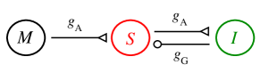
(b)

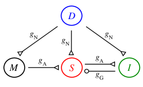
Figure 1: (a) (Color online) Three neurons coupled by chemical synapses in the master-slave-interneuron (MSI) configuration : excitatory AMPA synapses (with maximal conductance $g_{A}$) couple master (M) to slave (S) and slave to interneuron (I), whereas an inhibitory GABA${}_{\text{A}}$ synapse (with maximal conductance $g_{G}$) couples interneuron to slave. (b) Same as (a), except that all three neurons of the MSI circuit receive excitatory (NMDA) synapses from a driver neuron (D).

As we show in section III below, whether or not the MSI circuit can exhibit AS depends, among other factors, on the excitability of the three neurons. In the MSI, this is controlled by a constant applied current (see section III.1). To test the robustness of the results (and at the same time improve the realism and complexity of the model), in section III.2 we study the four-neuron motif depicted in Fig. 1b, where the excitability of the MSI network is chemically modulated via synapses projecting from a global driver ($D$). From now on, we refer to the 4-neuron motif as a Driver-Master-Slave-Interneuron (DMSI) microcircuit.

II.2 Model neurons

In the above networks, each node is described by a Hodgkin-Huxley (HH) model neuron HH52 , consisting of four coupled ordinary differential equations associated to the membrane potential $V$ and the ionic currents flowing across the axonal membrane corresponding to the Na, K and leakage currents. The gating variables for sodium are $h$ and $m$ and for the potassium is $n$. The equations read Koch :

$$C_{m}\frac{dV}{dt} = \overline{G}_{Na}m^{3}h(E_{Na}-V)+\overline{G}_{K}n^{4}(E_{K}-V)$$ (2)

$$+G_{m}(V_{rest}-V)+I+\sum I_{syn}$$

$$\frac{dx}{dt} = \alpha_{x}(V)(1-x)-\beta_{x}(V)x\;,$$ (3)

where $x\in\{h,m,n\}$, $C_{m}=9\pi$ $\mu$F is the membrane capacitance of a $30\times 30\times\pi$ $\mu$m² equipotential patch of membrane Koch , $I$ is a constant current which sets the neuron excitability and $\sum I_{syn}$ accounts for the interaction with other neurons. The reversal potentials are $E_{Na}=115$ mV, $E_{K}=-12$ mV and $V_{rest}=10.6$ mV, which correspond to maximal conductances $\overline{G}_{Na}=1080\pi$ mS, $\overline{G}_{K}=324\pi$ mS and $G_{m}=2.7\pi$ mS, respectively. The voltage dependent rate constants in the Hodgkin-Huxley model have the form:

$$\alpha_{n}(V) = \frac{10-V}{100(e^{(10-V)/10}-1)},$$ (4)

$$\beta_{n}(V) = 0.125e^{-V/80},$$ (5)

$$\alpha_{m}(V) = \frac{25-V}{10(e^{(25-V)/10}-1)},$$ (6)

$$\beta_{m}(V) = 4e^{-V/18},$$ (7)

$$\alpha_{h}(V) = 0.07e^{-V/20},$$ (8)

$$\beta_{h}(V) = \frac{1}{(e^{(30-V)/10}+1)}.$$ (9)

Note that all voltages are expressed relative to the resting potential of the model at $I=0$ Koch .

According to Rinzel and Miller Rinzel80 , in the absence of synaptic currents the only attractor of the system of equations (2)-(9) for $I\lesssim 177.13$ pA is a stable fixed point, which loses stability via a subcritical Hopf bifurcation at $I\simeq 276.51$ pA. For $177.13$ pA $\lesssim I\lesssim 276.51$ pA, the stable fix point coexists with a stable limit cycle.

II.3 Synaptic coupling

AMPA (A) and GABA${}_{\text{A}}$ (G) are the fast excitatory and inhibitory synapses in our model [see Fig. 1a]. Following Destexhe et al KochSegev , the fraction $r^{(i)}$ ($i=A,G$) of bound (i.e. open) synaptic receptors is modelled by a first-order kinetic dynamics:

$$\frac{dr^{(i)}}{dt}=\alpha_{i}[T](1-r^{(i)})-\beta_{i}r^{(i)},$$ (10)

where $\alpha_{i}$ and $\beta_{i}$ are rate constants and $[T]$ is the neurotransmitter concentration in the synaptic cleft. For simplicity, we assume $[T]$ to be an instantaneous function of the pre-synaptic potential $V_{pre}$:

$$[T](V_{pre})=\frac{T_{max}}{1+e^{[-(V_{pre}-V_{p})/K_{p}]}},$$ (11)

where $T_{max}=1$ mM^-1 is the maximal value of $[T]$, $K_{p}=5$ mV gives the steepness of the sigmoid and $V_{p}=62$ mV sets the value at which the function is half-activated KochSegev .

The synaptic current at a given synapse is given by

$$I^{(i)}=g_{i}r^{(i)}(V-E_{i}),$$ (12)

where $V$ is the postsynaptic potential, $g_{i}$ the maximal conductance and $E_{i}$ the reversal potential. We use $E_{A}=60$ mV and $E_{G}=-20$ mV.

The values of the rate constants $\alpha_{A}$, $\beta_{A}$, $\alpha_{G}$, and $\beta_{G}$ are known to depend on a number of different factors and vary significantly Geiger97 ; Geiger02 ; Hausser97 ; Kraushaar00 . To exemplify some of our results, we initially fix some parameters, which are set to the values of Table 1 unless otherwise stated (section III.1.1). Then we allow these parameters (as well as the synaptic conductances) to vary within the physiological range when exploring different synchronization regimes (see section III.1.2 and III.2).

	$MSI$	$DMSI$
$\alpha_{A}$ (mM-1ms-1)	$1.1$	$1.1$
$\beta_{A}$ (ms-1)	$0.19$	$0.19$
$\alpha_{G}$ (mM-1ms-1)	$5.0$	$5.0$
$\beta_{G}$ (ms-1)	$0.30$	$0.60$
$\alpha_{N}$ (mM-1ms-1)	—	$0.072$
$\beta_{N}$ (ms-1)	—	$0.0066$
$g_{A}$ (nS)	$10$	$10$
$I$ (pA)	$280$	$160$

Table 1: Standard values employed in the model. See text for details.

The slow excitatory synapse is NMDA (N) and its synaptic current is given by:

$$I^{(N)}=g_{N}B(V)r^{(N)}(V-E_{N}),$$ (13)

where $E_{N}=60$ mV. The dynamics of the variable $r^{(N)}$ is similar to eq. (10) with $\alpha_{N}=0.072$ mM^-1ms^-1 and $\beta_{N}=0.0066$ ms^-1. The magnesium block of the NMDA receptor channel can be modeled as a function of postsynaptic voltage $V$:

$$B(V)=\frac{1}{1+e^{(-0.062V)[\text{Mg}^{2+}]_{o}/3.57}},$$ (14)

where $[\text{Mg}^{2+}]_{o}=1$ mM is the physiological extracellular magnesium concentration.

In what follows, we will drop the neurotransmitter superscripts $A$, $G$ and $N$ from the synaptic variables $r$ and $I$. Instead we use double subscripts to denote the referred pre- and postsynaptic neurons. For instance, the synaptic current in the slave neuron due to the interneuron (the only inhibitory synapse in our models) will be denoted as $I_{IS}$, and so forth.

III Results

III.1 Master-Slave-Interneuron circuits

III.1.1 Three dynamical regimes

Initially, we describe results for the scenario where all neurons receive a constant current $I\geqslant 280$ pA. This corresponds to a situation in which the fixed points are unstable and, when isolated, they spike periodically. All other parameters are as in Table 1. For different sets of inhibitory conductance values $g_{G}$ our system can exhibit three different behaviors. To characterize them, we define $t^{M}_{i}$ as the time the membrane potential of the master neuron is at its maximal value in the $i$-th cycle (i.e. its $i$-th spike time), and $t_{i}^{S}$ as the spike time of the slave neuron which is nearest to $t_{i}^{M}$.

The delay $\tau_{i}$ is defined as the difference (see Fig. 2):

$$\tau_{i}\equiv t^{M}_{i}-t^{S}_{i}.$$ (15)

Initial conditions were randomly chosen for each computed time series. When $\tau_{i}$ converges to a constant value $\tau$, a phase-locked regime is reached Strogatz . If $\tau<0$ (“master neuron spikes first”) we say that the system exhibits delayed synchronization (DS) [Fig. 2(a)]. If $\tau>0$ (“slave neuron spikes first”), we say that anticipated synchronization (AS) occurs [Fig. 2(b)]. If $\tau$ does not converge to a fixed value, the system is in a phase drift (PD) regime Strogatz . The extent to which the AS regime can be legitimately considered “anticipated” in a periodic system will be discussed below.

(a)

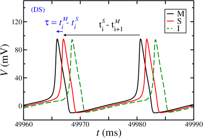
(b)

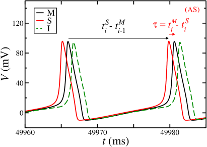
Figure 2: (Color online) Membrane potential $V$ as a function of time for an external current $I=280$ pA in the master (M), slave (S), and interneuron (I) neurons. The plot illustrates two regimes: (a) $g_{G}=20$ nS leads to delayed synchronization (DS), where $\tau<0$, and (b) $g_{G}=40$ nS leads to anticipated synchronization (AS), where $\tau>0$. Other parameters as in Table 1.

(a) DS

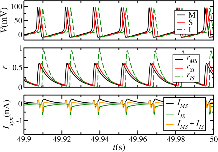
(b) AS

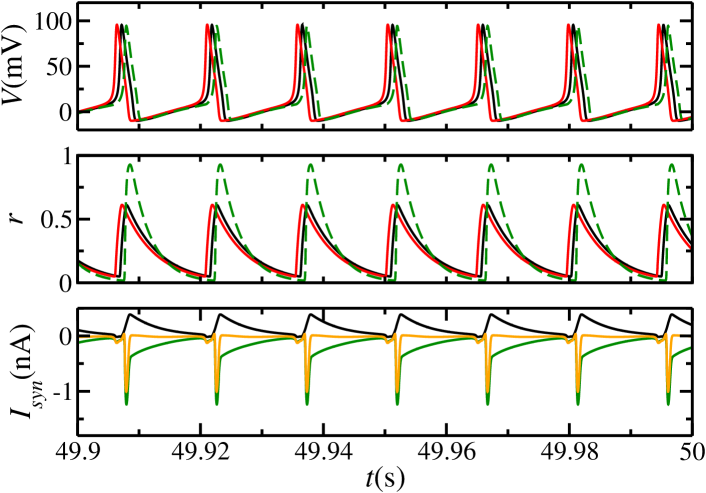
(c) PD

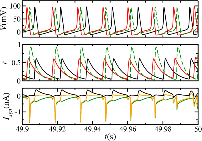
Figure 3: (Color online) Time series of the membrane potentials ($V$), bound receptors ($r$) and synaptic currents ($I$), with model parameters as in Table 1. Note that the system is periodic in the DS and AS regimes [(a) and (b) respectively], but not in the PD regime (c).

In Figure 3 we show examples of time series in the three different regimes (DS, AS and PD). The different panels correspond to the membrane potential, fraction of activated receptors for each synapse, and synaptic current in the slave neuron. For a relatively small value of the inhibitory coupling [$g_{G}=20$ nS, Fig. 3(a)] the slave neuron lags behind the master, characterizing DS. In Fig. 3(b), we observe that by increasing the value of the inhibitory coupling ($g_{G}=40$ nS) we reach an AS regime. Finally, for strong enough inhibition [$g_{G}=60$ nS, Fig. 3(c)] the PD regime ensues.

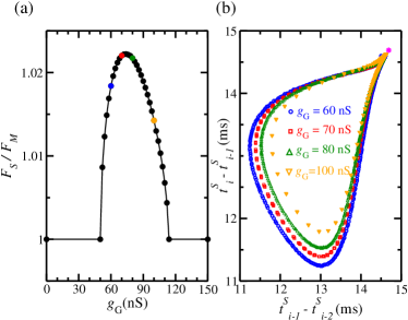
Figure 4: (Color online) (a) The mean firing rate of the slave ($F_{S}$) coincides with the mean firing rate of the master ($F_{M}$) for DS and AS regimes, but it is larger for PD. (b) In PD, the return map of the inter-spike interval of the slave is consistent with a quasi-periodic system (the pink star shows the return map of the master).

In the DS and AS regimes the master and slave neurons spike at the same frequency. However, when the system reaches the PD regime the mean firing rate of the slave neuron becomes higher than that of the master. The counterintuitive result shown in Fig. 4(a) emerges: the mean firing rate of the slave neuron increases while increasing the conductance of the inhibitory synapse projected from the interneuron. For the particular combination of parameters used in Fig. 4(a), the transition turns out to be reentrant, i.e., the system returns to the DS regime for sufficiently strong inhibition (a more detailed exploration of parameter space will be presented below). Figure 4(b) shows the return map of the inter-spike interval of the slave, which forms a closed curve (touching the trivial single-point return map of the master). This is consistent with a quasi-periodic phase-drift regime.

Note that in this simple scenario $g_{G}$ plays an analogous role to that of $K$ in Eq. 1, for which AS is stable only when $K>K_{c}$ (eventually with reentrances) Toral03 . Moreover, the behavior of the synaptic current in the slave neuron is particularly revealing: in the DS regime [Fig. 3(a)], it has a positive peak prior to the slave spike, which drives the firing in the slave neuron. In the AS regime [Fig. 3(b)], however, there is no significant resulting current, except when the slave neuron is already suprathreshold. In this case, the current has essentially no effect upon the slave dynamics. This situation is similar to the stable anticipated solution of Eq. 1, when the coupling term vanishes.

III.1.2 Scanning parameter space

The dependence of the time delay $\tau$ on $g_{G}$ is shown in Fig. 5 for different values of the external current $I$ and maximal excitatory conductance $g_{A}$. Several features in those curves are worth emphasizing. First, unlike previous studies on AS, where the anticipation time was hardwired via the delay parameter $t_{d}$ [see eq.(1)], in our case the anticipation time $\tau$ is a result of the dynamics. Note that $g_{G}$ (the parameter varied in Fig. 5) does not change the time scales of the synaptic dynamical variables ($r$), only the synaptic strength.

Secondly, $\tau$ varies smoothly with $g_{G}$. This continuity somehow allows us to interpret $\tau>0$ as a legitimately anticipated regime. The reasoning is as follows. For $g_{G}=0$, we simply have a master-slave configuration in which the two neurons spike periodically. Due to the excitatory coupling, the slave’s spike is always closer to the master’s spike which preceded it than to the master’s spike which succeeded it [as in e.g. Fig. (2)(a)]. Moreover, the time difference is approximately $1.5$ ms, which is comparable to the characteristic times of the synapse. In that case, despite the formal ambiguity implicit in the periodicity of the time series, the dynamical regime is usually understood as “delayed synchronization”. We interpret it in the following sense: the system is phase-locked at a phase difference with a well defined sign Strogatz . Increasing $g_{G}$, the time difference between the master’s and the slave’s spikes eventually changes sign [as in e.g. Fig. (2)(b)]. Even though the ambiguity in principle remains, there is no reason why we should not call this regime “anticipated synchronization” (again a phase-locked regime, but with a phase difference of opposite sign). In fact, we have not found any parameter change which would take the model from the situation in Fig. (2)(a) to that of Fig. (2)(b) by gradually increasing the lag of the slave spike until it approached the next master spike. If that ever happened, $\tau$ would change discontinuously (by its definition). Therefore, the term “anticipated synchronization” by no means implies violation of causality and should just be interpreted with caution. As we will discuss in section IV, the relative timing between pre- and postsynaptic neurons turns out to be extremely relevant for real neurons.

Third, it is interesting to note that the largest anticipation time can be longer (up to $3$ ms, i.e. about $20\%$ of the interspike interval) than the largest time for the delayed synchronization ($\approx 1.5$ ms). If one increases $g_{G}$ further in an attempt to obtain even larger values of $\tau$, however, the system undergoes a bifurcation to a regime with phase drift [which marks the end of the curves in Fig. 5].

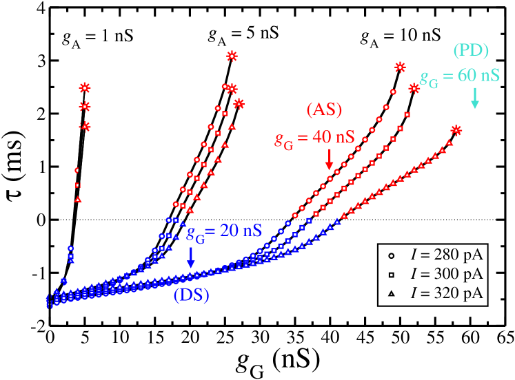
Figure 5: (Color online) Dependence of the time delay $\tau$ with the maximal conductance $g_{G}$ for different values of the applied current $I$ and $g_{A}$. The end of each curve (stars) marks the critical value of $g_{G}$, above which the system changes from AS to PD.

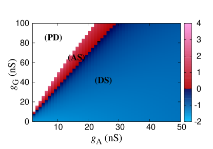
Figure 6: (Color online) Delay $\tau$ (right bar) in the $(g_{A},g_{G})$ projection of parameter space: DS (blue, right), AS (red, middle) and PD (white, left — meaning that no stationary value of $\tau$ was found).

The number of parameters in our model is very large. The number of dynamical regimes which a system of coupled nonlinear oscillators can present is also very large, most notably $p/q$-subharmonic locking structured in Arnold tongues Nayfeh . These occur in our model, but not in the parameter region we are considering. In this context, an attempt to map all the dynamical possibilities in parameter space would be extremely difficult and, most important, improductive for our purposes. We therefore focus on addressing the main question of this paper, which is whether or not AS can be stable in a biophysically plausible model.

In Fig. 6 we display a two-dimensional projection of the phase diagram of our model. We employ the values in Table 1, except for $g_{A}$, which is varied along the horizontal axis. Note that each black curve with circles in Fig. 5 corresponds to a different vertical cut of Fig. 6, along which $g_{G}$ changes. We observe that the three different regimes are distributed in large continuous regions, having a clear transition between them. Moreover the transition from the DS to the AS phase can be well approximated by a linear relation $g_{G}/g_{A}\approx 3.5$ in a large portion of the diagram.

Figure 7: (Color online) Delay $\tau$ (right bar) in the $(g_{A},g_{G})$ projection of parameter space for different combinations of $\beta_{A}$ and $\beta_{G}$. From left to right we have respectively PD, AS and DS regimes, as in Fig. 6.

Linearity, however, breaks down as parameters are further varied. This can be seen e.g. in Fig. 7, which displays the same projection as Fig. 6, but for different combinations of $\beta_{G}$ and $\beta_{A}$. We observe that AS remains stable in a finite region of the parameter space, and this region increases as excitatory synapses become faster.

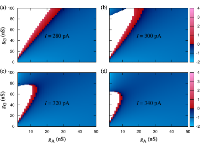
Figure 8: (Color online) Delay $\tau$ (right bar) in the $(g_{A},g_{G})$ projection of parameter space for different values of $I$. PD, AS and DS regimes as in Fig. 6.

Figure 5 suggests that larger values of the input current $I$ eventually lead to a transition from AS from DS. This effect is better depicted in Fig. 8, where the DS region increases in size as $I$ (and therefore the firing rate) increases. Figures 8(b)-(d) also show that the system can exhibit reentrant transitions as $g_{G}$ is varied. Most importantly, however, is that Figs. 7 and 8 show that there is always an AS region in parameter space, as synaptic and intrinsic parameters are varied.

As we will discuss in section IV, the possibility of controlling the transition between AS and DS is in principle extremely appealing to the study of plasticity in neuroscience. However, in a biological network, the input current would not be exactly constant, but rather be modulated by other neurons. In the following, we test the robustness of AS in this more involved scenario, therefore moving one step ahead in biological plausibility.

III.2 Driver-Master-Slave-Interneuron circuits

Let us consider the MSI circuit under a constant input current $I=160$ pA. This is below the Hopf bifurcation Rinzel80 , i.e. none of the three neurons spikes tonically. Their activity will now be controlled by the driver neuron (D), which projects excitatory synapses onto the MSI circuit [see Fig. 1(b)]. We chose to replace the constant input current by a slowly varying current, so that the synapses projecting from the driver neuron are of the NMDA type (see section II). The driver neuron receives a current $I_{D}=280$ pA, so it spikes tonically. All remaining parameters are as in the second column of Table 1. The interest in this case is to verify whether AS holds when the excitability of the MSI circuit is modulated by a non-stationary current.

As shown in Fig. 9, we found in this new scenario a similar route from DS to AS, and then the PD regime (compare with Fig. 7). Note that the characteristic time ($\beta_{N}=6.6$ s^-1) for the unbinding of the NMDA receptors is about ten times larger than the inter-spike interval of the driver neuron (which spikes at $\approx 67$ Hz). As a consequence, $r_{DM}$, $r_{DS}$, $r_{DI}$ are kept at nearly constant values (with variations of $\approx 10\%$ around a mean value — data not shown). The variations in the NMDA synaptic current are also small, which in principle should make the system behave in an apparently similar way to the previous MSI circuit. However, these small variations are important enough to increase the AS domain in parameter space, in some cases even eliminating the PD region (see e.g. Fig. 9 for $\beta_{G}=0.30$ ms^-1). Therefore, at least in this case, the use of more biological plausible parameters does not destroy AS, but rather enhances it.

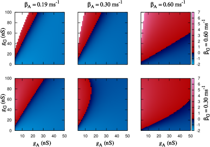
Figure 9: (Color online) DMSI circuit (see Fig. 1b). Delay $\tau$ (right bar) in the $(g_{A},g_{G})$ projection of parameter space for different combinations of $\beta_{A}$ and $\beta_{G}$. PD, AS and DS regimes as in Fig. 6.

Figure 10: (Color online) DMSI circuit (see Fig. 1b). (a) The mean firing rate of the slave ($F_{S}$) coincides with the mean firing rate of the master ($F_{M}$) for DS and AS regimes, but it is larger for PD. (b) In PD, the return map of the inter-spike interval of the slave is consistent with a quasi-periodic system.

In fact, the three regions in the MSI diagrams seem to retain their main features in the DMSI circuit. When PD occurs, for example, the slave again spikes faster than the master [Fig. 10(a)], like in the MSI circuit [compare with Fig. 4(a)]. Another signature of the robustness of the PD phase against the replacement of a constant by a slowly-varying synaptic current appears in the return map shown in Fig. 10(b). It can be seen that it has the same structure of its three-neuron counterpart shown in Fig. 4(b).

IV Concluding remarks

In summary, we have shown that a biologically plausible model of a 3-neuron (MSI) motif can exhibit an attractor in phase space where anticipated synchronization is stable. The transition from the DS to the AS regime is a smooth function of the synaptic conductances. Typically, a further increase in the inhibitory conductance $g_{G}$ leads to a second transition from AS to PD, a quasiperiodic regime in which the slave firing frequency is larger than that of the master.

We have varied synaptic decay rates ($\beta$), synaptic conductances ($g$) as well as input currents ($I$) within well accepted physiological ranges Geiger97 ; Geiger02 ; Hausser97 ; Kraushaar00 . In all the scenarios there is always a continuous region in parameter space where AS is stable. Replacing the constant current by a global periodic driver (arguably a more realistic situation), we obtain a model of a 4-neuron (DMSI) motif which exhibits the same three regions of the simpler model. The synaptic rise constants ($\alpha$) were also varied, but have a lesser effect on the transitions among the different regimes (data not shown). Therefore the phenomenon seems to be robust at the microcircuit scale.

It is important to emphasize that our AS results differ from those obtained from eq. (1) at a fundamental level. In our model the delayed feedback that leads to AS is given by biologically plausible elements (an interneuron and chemical synapses). Hence, the anticipation time is not hard-wired in the dynamical equations, but rather emerges from the circuit dynamics. Moreover, the particular circuit we study is a neuronal motif ubiquitously found in the brain Shepherd ; thalamus1 ; thalamus2 . We are unaware of other AS models in which every parameter has a clear biological interpretation.

We believe that our results can be extremely relevant for modeling studies of synaptic plasticity. Recent decades have witnessed a growing literature on spike-timing dependent plasticity (STDP), which accounts for the enhancement or diminution of synaptic weight [long term potentiation (LTP) and long term depression (LTD), respectively] depending on the relative timing between the spikes of the pre- and post-synaptic neurons (see e.g. Abbott00 ; Gerstner ; Clopath10 ). Experimental data strongly suggest that if the pre-synaptic neuron fires before (after) the post-synaptic neuron, the synapse between them will be strenghtened (weakened) Markram97 ; Bi98 . STDP is supposed to take place in a window of time differences between post- and pre-synaptic spikes in the order of ten milliseconds, within which the delay and anticipation times of our models fall. Since the DS-AS transition amounts to an inversion in the timing of the pre- and post-synaptic spikes, then by appropriately controlling this effect one could dynamically toggle between synaptic strengthening and weakening. This could be potentially linked with modeling of large-scale ascending feedback modulation from reward systems.

Our results, therefore, offer a number of possibilities for further investigation. Including effects from microcircuit dynamics (such as the ones we have presented here) in models of synaptic plasticity is a natural next step, one which we are currently pursuing. Once we have verified AS in a biologically plausible model, one could consider using simplified models Neiman99 ; Izhikevich06 (e.g. by replacing the HH equations and/or the synaptic kinetics) and the influence of noise Ciszak03 ; Koch . We are also investigating whether the structure of the phase diagram can be qualitatively reproduced via a phase-response-curve analysis Ermentrout96 ; Rinzel98b of the neuronal motifs studied here. Results will be published elsewhere.

- (1) S. Boccaletti, J. Kurths, G. Osipov, D. L. Valladares, and C. S. Zhou, Phys. Rep. 366, 1 (2002)
- (2) H. U. Voss, Phys. Rev. E 61, 5115 (2000)
- (3) H. U. Voss, Phys. Rev. E 64, 039904 (2001)
- (4) H. U. Voss, Phys. Rev. Lett. 87, 014102 (2001)
- (5) M. Kostur, P. Hänggi, P. Talkner, and J. L. Mateos, Phys. Rev. E 72, 036210 (2005)
- (6) C. Masoller and D. H. Zanette, Physica A 300, 359 (2001)
- (7) S. Sivaprakasam, E. M. Shahverdiev, P. S. Spencer, and K. A. Shore, Phys. Rev. Lett. 87, 154101 (2001)
- (8) Y. Liu, Y. Takiguchi, P. Davis, T. Aida, and S. Saito, Appl. Phys. Lett. 80, 4306 (2002)
- (9) M. Ciszak, C. R. Mirasso, R. Toral, and O. Calvo, Phys. Rev. E 79, 046203 (2009)
- (10) M. Ciszak, O. Calvo, C. Masoller, C. R. Mirasso, and R. Toral, Phys. Rev. Lett. 90, 204102 (May 2003)
- (11) M. Ciszak, F. Marino, R. Toral, and S. Balle, Phys. Rev. Lett. 93, 114102 (2004)
- (12) R. Toral, C. Masoller, C. R. Mirasso, M. Ciszak, and O. Calvo, Physica A 325, 192 (2003)
- (13) Essentials of Neural Science and Behavior, edited by E. R. Kandel, J. H. Schwartz, and T. M. Jessell (Appleton & Lange, Norwalk, 1995)
- (14) A. Arvanitaki, J. Neurophysiol 5, 89 (1942)
- (15) The Synaptic Organization of the Brain, edited by G. M. Shepherd (Oxford University Press, New York, 1998)
- (16) U. Kim, M. V. Sanchez-Vives, and D. A. McCormick, Science 278, 130 (1997)
- (17) D. Debay, J. Wolfart, Y. Le Franc, G. Le Masson, and T. Bal, J. Physiol., 540(2004)
- (18) G. B. Mindlin and R. Laje, The Physics of Birdsong (Springer, 2005)
- (19) A. L. Hodgkin and A. F. Huxley, J. Neurophysiol. 117, 500 (1952)
- (20) C. Koch, Biophysics of Computation (Oxford University Press, New York, 1999)
- (21) J. Rinzel and R. N. Miller, Math. Biosci. 49, 27 (1980)
- (22) Methods in Neuronal Modeling: From Ions to Networks, 2nd ed., edited by C. Koch and I. Segev (MIT Press, 1998)
- (23) J. R. P. Geiger, J. Lübke, A. Roth, M. Frotscher, and P. Jonas, Neuron 18, 1009 (1997)
- (24) M. Bartos, I. Vida, M. Frotscher, A. Meyer, H. Monyer, J. R. P. Geiger, and P. Jonas, Proc. Natl. Acad. Sci. 99, 13222 (2002)
- (25) M. Hausser and A. Roth, J. Neurosci. 17, 7606 (1997)
- (26) U. Kraushaar and P. Jonas, J. Neurosci. 20, 5594 (2000)
- (27) S. H. Strogatz, Nonlinear Dynamics and Chaos: with Applications to Physics, Biology, Chemistry and Engineering (Addison-Wesley, Reading, MA, 1997)
- (28) R. Toral, C. R. Mirasso, and J. D. Gunton, Europhys. Lett. 61, 162 (2003)
- (29) A. H. Nayfeh and D. T. Mook, Nonlinear oscillators (John Wiley & Sons, New York, 1979)
- (30) L. F. Abbott and S. B. Nelson, Nat Neurosci. 3, 1178 (2000)
- (31) W. Gerstner and W. Kistler, Spiking Neuron Models: Single Neurons, Populations, Plasticity (Cambridge University Press, 2002)
- (32) C. Clopath, L. Büsing, E. Vasilaki, and W. Gerstner, Nat. Neurosci. 13, 344 (2010)
- (33) H. Markram, J. Lübke, M. Frotscher, and B. Sakmann, Science 275, 213 (1997)
- (34) G. Q. Bi and M. M. Poo, J. Neurosci. 18, 10464 (1998)
- (35) A. Neiman, X. Pei, D. Russell, W. Wojtenek, L. Wilkens, F. Moss, H. A. Braun, M. T. Huber, and K. Voigt, Phys. Rev. Lett. 82, 660 (Jan 1999)
- (36) E. M. Izhikevich, Dynamical Systems in Neuroscience: The Geometry of Excitability and Bursting (MIT Press, Cambridge, 2006)
- (37) G. B. Ermentrout, Neural Comput. 8, 979 (1996)
- (38) J. Rinzel and B. Ermentrout, in Methods in Neuronal Modeling: From Ions to Networks, edited by C. Koch and I. Segev (MIT Press, 1998) 2nd ed., pp. 251–292