A Combined Optical and X-ray Study of Unobscured Type 1 AGN. I. Optical Spectra and SED Modeling

Abstract

We present modeling and interpretation of the continuum and emission lines for a sample of 51 unobscured Type 1 active galactic nuclei (AGN). All of these AGNs have high quality spectra from both XMM-Newton and Sloan Digital Sky Survey (SDSS). We extend the wavelength coverage where possible by adding simultaneous UV data from the OM onboard XMM-Newton. Our sample is selected based on low reddening in the optical and low gas columns implied by their X-ray spectra, except for one case, the BAL-quasar PG 1004+130. They also lack clear signatures for the presence of a warm absorber. Therefore the observed characteristics of this sample are likely to be directly related to the intrinsic properties of the central engine.

To determine the intrinsic optical continuum we subtract the Balmer continuum and all major emission lines (including FeII). We also consider possible effects of contamination from the host galaxy. The resulting continuum is then used to derive the properties of the underlying accretion disc. We constrain the black hole masses from spectral fits of the Balmer emission lines and determine the best fit value from the modeling of broadband spectral energy distributions (SED). In addition to the disc component, many of these SEDs also exhibit a strong soft X-ray excess, plus a power law extending to higher X-ray energies. We fit these SEDs by applying a new broadband SED model which comprises the accretion disc emission, low temperature optically thick Comptonisation and a hard X-ray tail by introducing the concept of a corona radius (Done et al. 2011). We find that in order to fit the data, the model often requires an additional long wavelength optical continuum component, whose origin is discussed in this paper. We also find that the Photo-recombination edge of Balmer continuum shifts and broadens beyond the standard limit of 3646Å, implying an electron number density which is far higher than that in the broad line region clouds.

Our results indicate that the Narrow Line Seyfert 1s in this sample tend to have lower black hole masses, higher Eddington ratios, softer 2-10 keV band spectra, lower 2-10 keV luminosities and higher $\alpha_{ox}$, compared with typical broad line Seyfert 1s (BLS1), although their bolometric luminosities are similar. We illustrate these differences in properties by forming an average SED for three subsamples, based on the FWHM velocity width of the H$\beta$ emission line.

1 Introduction

The spectral energy distribution (SED) of AGN has been modeled for several decades. Initial studies focused on the infrared, optical and ultraviolet continuum (e.g. Wills et al. 1985; Canalizo & Stockton 2001; Lacy et al. 2007). With the inclusion of X-ray data, it was possible to define the continuum on both sides of the ultraviolet/X-ray gap (imposed by galactic photoelectric absorption), and so constrain the properties of the accretion disc (e.g. Ward et al. 1987; Elvis et al. 1994). Refinements to modeling the optical/UV continuum include subtraction of the complex blended features arising from permitted iron emission, the so-called small blue-bump from the Balmer continuum, and contamination across the entire spectrum from a stellar component (Maoz et al. 1993; Boisson et al. 2000)

The observed spectral differences between various types of AGN are not only due to selective absorption and orientation effects, as implied by the simplest version of AGN unification model (Antonucci 1993), but also result from a wide range in basic physical parameters, such as black hole mass and accretion rate (e.g. Boroson & Green 1992; Boller, Brandt & Fink 1996; Done & Gierliński 2005; Zhou et al. 2006). To better understand the accretion processes occurring close to the super massive black hole (SMBH), we construct broadband SEDs. Galactic dust reddening, together with the intrinsic reddening of the AGN itself, attenuates the optical/UV band emission. Furthermore, Photoelectric absorption from gas modifies the lower energy X-ray continuum. But these factors can be quantified and corrected. Thereby we can recover the intrinsic SED, except for the unobservable far-UV region. If we have reliable data on both sides of the energy gap between the UV and soft X-ray, we can apply a multi-component model which spans across it.

Table 1: The Seyfert 1 Galaxy Sample Set

			2XMMi Catalog	XMM-Newton	SDSS DR7	SDSS	EPIC
ID	Common Namea	Redshift	IAU Name (2XMMb)	Obs Date	MJD-Plate-Fibre	Obs Date	Countsc
1	UM 269	0.308	J004319.7+005115	2002-01-04	51794-0393-407	2000-09-07	19126
2	MRK 1018	0.043	J020615.9-001730	2005-01-15	51812-0404-141	2000-09-25	2056
3	NVSS J030639	0.107	J030639.5+000343	2003-02-11	52205-0709-637	2001-10-23	35651
4	2XMMi/DR7	0.145	J074601.2+280732	2001-04-26	52618-1059-399	2002-12-10	9679
5	2XMMi/DR7	0.358	J080608.0+244421	2001-10-26	52705-1265-410	2003-03-07	2912
6	HS 0810+5157	0.377	J081422.1+514839	2003-04-27	53297-1781-220	2004-10-19	4189
7	RBS 0769	0.160	J092246.9+512037	2005-10-08	52247-0766-614	2001-12-04	32731
8	RBS 0770	0.033	J092342.9+225433∗	2006-04-18	53727-2290-578	2005-12-23	104028
9	MRK 0110	0.035	J092512.8+521711	2004-11-15	52252-0767-418	2001-12-09	515453
10	PG 0947+396	0.206	J095048.3+392650	2001-11-03	52765-1277-332	2003-05-06	58555
11	2XMMi/DR7	0.373	J100025.2+015852	2003-12-10	52235-0501-277	2001-11-22	7187
12	2XMMi/DR7	0.206	J100523.9+410746	2004-04-20	52672-1217-010	2003-02-02	5437
13	PG 1004+130	0.241	J100726.0+124856	2003-05-04	53055-1744-630	2004-02-20	3781
14	RBS 0875	0.178	J103059.0+310255	2000-12-06	53440-1959-066	2005-03-11	69434
15	KUG 1031+398	0.043	J103438.6+393828	2002-05-01	53002-1430-485	2003-12-29	63891
16	PG 1048+342	0.160	J105143.8+335927	2002-05-13	53431-2025-637	2005-03-02	47858
17	1RXS J111007	0.262	J111006.8+612522∗	2006-11-25	52286-0774-600	2002-01-12	6147
18	PG 1115+407	0.155	J111830.2+402554	2002-05-17	53084-1440-204	2004-03-20	64601
19	2XMMi/DR7	0.101	J112328.0+052823	2001-12-15	52376-0836-453	2002-04-12	10098
20	RX J1140.1+0307	0.081	J114008.7+030710	2005-12-03	51994-0514-331	2001-03-26	35616
21	PG 1202+281	0.165	J120442.1+275412	2002-05-30	53819-2226-585	2006-03-25	66550
22	1AXG J121359+1404	0.154	J121356.1+140431	2001-06-15	53466-1765-058	2005-04-06	12975
23	2E 1216+0700	0.080	J121930.9+064334	2002-12-18	53140-1625-134	2004-04-26	8028
24	1RXS J122019	0.286	J122018.4+064120	2002-07-05	53472-1626-292	2005-04-12	8338
25	LBQS 1228+1116	0.236	J123054.1+110011	2005-12-17	52731-1232-417	2003-04-02	165823
26	2XMMi/DR7	0.304	J123126.4+105111	2005-12-17	52731-1232-452	2003-04-02	8816
27	MRK 0771	0.064	J123203.6+200929	2005-07-09	54481-2613-342	2008-01-15	40705
28	RX J1233.9+0747	0.371	J123356.1+074755	2004-06-05	53474-1628-394	2005-04-14	6041
29	RX J1236.0+2641	0.209	J123604.0+264135∗	2006-06-24	53729-2236-255	2005-12-25	17744
30	PG 1244+026	0.048	J124635.3+022209	2001-06-17	52024-0522-173	2001-04-25	8509
31	2XMMi/DR7	0.316	J125553.0+272405	2000-06-21	53823-2240-195	2006-03-26	7591
32	RBS 1201	0.091	J130022.1+282402	2004-06-06	53499-2011-114	2005-05-09	209458
33	2XMMi/DR7	0.334	J132101.4+340658	2001-01-09	53851-2023-044	2006-04-26	4425
34	1RXS J132447	0.306	J132447.6+032431	2004-01-25	52342-0527-329	2002-03-09	6305
35	UM 602	0.237	J134113.9-005314	2005-06-28	51671-0299-133	2000-05-07	18007
36	1E 1346+26.7	0.059	J134834.9+263109	2000-06-26	53848-2114-247	2006-04-23	71985
37	PG 1352+183	0.151	J135435.6+180518	2002-07-20	54508-2756-228	2008-02-12	36171
38	MRK 0464	0.050	J135553.4+383428	2002-12-10	53460-2014-616	2005-03-31	13974
39	1RXS J135724	0.106	J135724.5+652506	2005-04-04	51989-0497-014	2001-03-21	12081
40	PG 1415+451	0.114	J141700.7+445606	2002-12-08	52728-1287-296	2003-03-30	55786
41	PG 1427+480	0.221	J142943.0+474726	2002-05-31	53462-1673-108	2005-04-01	70995
42	NGC 5683	0.037	J143452.4+483943	2002-12-09	52733-1047-300	2003-04-04	18885
43	RBS 1423	0.208	J144414.6+063306	2005-02-11	53494-1829-464	2005-05-04	37568
44	PG 1448+273	0.065	J145108.7+270926	2003-02-08	54208-2142-637	2007-04-18	134532
45	PG 1512+370	0.371	J151443.0+365050	2002-08-25	53083-1353-580	2004-03-14	40432
46	Q 1529+050	0.218	J153228.8+045358	2001-08-21	54563-1835-054	2008-04-07	10952
47	1E 1556+27.4	0.090	J155829.4+271715	2002-09-10	52817-1391-093	2003-06-27	6995
48	MRK 0493	0.031	J155909.6+350147	2003-01-16	53141-1417-078	2004-05-14	124115
49	II Zw 177	0.081	J221918.5+120753	2001-06-07	52221-0736-049	2001-11-08	36056
50	PG 2233+134	0.326	J223607.6+134355	2003-05-28	52520-0739-388	2002-09-03	7853
51	MRK 0926	0.047	J230443.3-084111	2000-12-01	52258-0725-510	2001-12-15	59513

^a for some targets without well-known names, we simply use ‘2XMMi/DR7’;

^b the full name should be ‘2XMM J…’, but for those targets with * symbol, their full names should be ‘2XMMi J…’;

^c the total counts in all three EPIC monitors, namely pn, MOS1 and MOS2, and there are at least 2000 counts in at least one

of these three monitors;

1.1 Previous Work

Many multi-wavelength studies have been carried out previously. Puchnarewicz et al. (1992) studied the optical properties of 53 AGNs in Córdova et al. (1992)’s sample with ultra soft X-ray excesses, and found that they tend to have narrower permitted lines than optically selected samples. Supporting this finding, Boller, Brandt & Fink (1996) studied ROSAT selected AGN with extremely soft X-ray spectra, and found that they tend to be Narrow-Line Seyfert 1s (NLS1s). Correspondingly they found that optically selected NLS1s often have large soft X-ray excesses. Walter & Fink (1993) combined soft X-ray and optical data for 58 Seyfert 1s, and showed that their broadband SED have a bump from UV to soft X-rays, which is now refered to as the big blue bump (BBB). Grupe et al. (1998) and Grupe et al. (1999) used a sample of 76 bright soft X-ray selected Seyferts with infrared data, optical spectra and soft X-ray spectra. Their results reinforced the connection between the optical and soft X-ray spectra, and confirmed the existence of strong BBB emission in these objects. Elvis et al. (1994) studied 47 quasars in a UV-soft X-ray sample, and derived the mean SEDs for radio-loud and radio-quiet sources. Recently, more detailed spectral models have been applied to broadband SEDs including simultaneous optical/UV and X-ray observations which avoid potential problems caused by variability. Vasudevan & Fabian (2007) (hereafter VF07) combined a disc and broken powerlaw model to fit optical, far UV and X-ray data for 54 AGN. They found a well-defined relationship between the hard X-ray bolometric correction and the Eddington ratio. Brocksopp et al. (2006) analysed the data from XMM-Newton’s simultaneous EPIC (X-ray) and OM (optical/UV) observations for 22 Palomar Green (PG) quasars. Another sample consisting of 21 NLS1s and 13 broad line AGNs was also defined using simultaneous data from XMM-Newton’s EPIC and OM monitor (Crummy et al. 2006). The SEDs of this sample were then fitted using various broadband SED models such as disc plus powerlaw model, disc reflection model and disc wind absorption model (Middleton, Done & Gierliński 2007). Vasudevan & Fabian (2009) derived SEDs using XMM-Newton’s simultaneous X-ray and optical/UV observations for 29 AGNs selected from Peterson et al. (2004)’s reverberation mapped sample. The well constrained black hole masses available for this sample enabled them to fit a better constrained accretion disc model, combined with a powerlaw, to the source’s broadband SEDs. Hence they derived more reliable Eddington ratios.

1.2 Our AGN Sample

In this paper we define an X-ray/optically selected sample of 51 AGN, all of which have low reddening (so excluding Seyfert 2s and 1.9/1.8s), to construct SEDs ranging from about 0.9 microns to 10 keV. We also apply corrections for the permitted iron features, the Balmer continuum and stellar contribution, in order to model the non-stellar continuum free from emission line effects. Included in this sample are a number of NLS1s, a subclass of AGN whose permitted line widths are comparable to those of forbidden lines. Their [OIII]$\lambda$5007/H$\beta$ ratio is also lower than the typical value of broad line Seyfert 1s (BLS1s) (Shuder & Osterbrock 1981; Osterbrock & Pogge 1985). For consistency with previous work, we classify AGNs in our sample as NLS1s if they have ratios of [OIII]$\lambda$5007/H$\beta<$ 3 and FWHM${}_{H\beta}<$ 2000 km/s (Goodrich 1989). We identify 10$\sim$12 NLS1s in our sample.

All objects in our sample have high quality optical spectra taken from the Sloan Digital Sky Survey (SDSS) DR7, X-ray spectra from the XMM-Newton EPIC cameras, and in some cases simultaneous optical/UV photometric data points from the XMM-Newton OM monitor. Combining these data reduces the impact of intrinsic variability and provides a good estimate of the spectral shape in the optical, near UV and X-ray regions. In addition, by analyzing the SDSS spectra, we can derive the parameters of the principal optical emission lines and underlying continuum. An important result from reverberation mapping study is the correlation between black hole mass, monochromatic luminosity at 5100 Å and H$\beta$ FWHM (e.g. Kaspi et al. 2000; Woo & Urry 2002; Peterson et al. 2004). We measure these quantities from the SDSS spectra, and then estimate black hole masses using this correlation.

Compared with previous work, a significant improvement of our study is that we employ a new broadband SED model which combines disc emission, Comptonisation and a high energy powerlaw component in the context of an energetically self-consistent model for the accretion disc emission (Done et al. 2011, also see Section 5.2). By fitting this model to our data, we can reproduce the whole broadband SED from the optical to X-ray. From this detailed SED fitting, we derive a number of interesting AGN properties such as: the bolometric luminosity, Eddington ratio, hard X-ray slope, and the hard X-ray bolometric correction. Combining all the broadband SED parameters with the optical parameters, we can provide further evidence for many previously suggested correlations, including all the correlations between optical and X-ray claimed in previous work, plus many others such as the H$\beta$ FWHM versus X-ray slope, black hole mass versus Eddington ratio, FeII luminosity versus [OIII]$\lambda$5007 emission line luminosity and the high excitation lines (e.g. [FeVII]$\lambda$6087, [FeX]$\lambda$6374) versus their ionizing flux (e.g. Boroson & Green 1992; Boller, Brandt & Fink 1996; Grupe et al. 1998; Grupe et al. 1999; Sulentic et al. 2000; Mullaney et al. 2009).

This paper is organized as follows. Section 2 describes the sample selection and data analysis procedures. The detailed spectral fitting methods and results including Balmer line fitting, optical spectral fitting and broadband SED fitting are each discussed in sections 3, 4 and 5, separately. We present the statistical properties of our sample in section 6. The summary and conclusions are given in section 7. A flat universe model with Hubble constant of $H_{0}=72$ km s^-1 Mpc^-1, $\Omega_{M}=0.27$ and $\Omega_{\Lambda}=0.73$ is adopted. In another paper, we will present our analysis of correlations between selected optical/UV emission features and the SED components, and discuss their physical implications (Jin et al. in prep., hereafter Paper II).

2 Sample Selection and Data Assembly

To identify a sample of Type 1 AGNs having both high quality X-ray and optical spectra, we performed a cross-correlation between 2XMMi catalog and SDSS DR7 catalog. We filtered the resulting large sample as described below. Our final sample consists of 51 Type 1 AGNs including 12 NLS1s, all with high quality optical and X-ray spectra and low reddening/absorption, and with H${\beta}$ line widths ranging from 600 $kms^{-1}$ up to 13000 $kms^{-1}$. All the sources are listed in Table 1.

2.1 The Cross-correlation of 2XMMi & SDSS DR7

The first step was to cross-correlate between 2XMMi and SDSS DR7 catalogs. The 2XMMi catalog contains 4117 XMM-Newton EPIC camera observations obtained between 03-02-2000 and 28-03-2008, and covering a sky area of $\sim$ 420 deg². The SDSS DR7 is the seventh data release of the Sloan sky survey. The SDSS spectroscopic data has sky coverage of $\sim$ 8200 deg², with spectra from 3800 Å to 9200 Å, and spectral resolution between 1800 and 2200.
Our cross-correlation consisted of three steps:
1. We first searched for all XMM/SDSS position pairs that lay within 20$\arcsec$ of each other, resulting in 5341 such cases.
2. For these 5341 unique X-ray sources, we imposed two further selection criteria: that source positions be separated by less than 3$\arcsec$, or that sources be separated by no more than 3 $\times$ the XMM-Newton position uncertainty and no more than 7$\arcsec$. This filtering resulted in 3491 unique X-ray sources. The 3$\arcsec$ separation is chosen because we want to include all possible XMM/SDSS pairs during these early filtering steps. From the 2XMMi and SDSS DR7 cross-correlation, there are 114 XMM/SDSS pairs whose separations are less than 3$\arcsec$, but are still nevertheless greater than 3 $\times$ the XMM position uncertainty. We included all of these pairs. The 7$\arcsec$ separation upper limit mitigates spurious matches, especially for fainter objects and/or those located far off-axis.
3. We selected only objects classified as extragalactic, giving a total of 3342 for further analysis.

2.2 Selection of Seyfert 1 with High Quality Spectra

Within these 3342 unique X-ray sources which satisfied all the above criteria, we applied further filtering to select only Type 1 AGNs having both high quality optical and X-ray spectra. The five steps in the filtering were as follows:
1. In order to obtain black hole mass estimates and also as reddening indicators, we require $H\beta$ and $H\alpha$ emission lines to be measurable. So we only selected sources with $H\beta$ in emission (as indicated by the SDSS $H\beta$ line models with at least 3$\sigma$ significance and $EW>0$) and redshift $z<0.4$. This selection resulted in 802 unique X-ray sources, and 888 XMM/SDSS pairs (since some X-ray objects were matched with more than one SDSS spectrum).
2. Then we searched for the Type 1 AGNs (including subtypes 1.0, 1.5, 1.8 and 1.9) which have a minimum of 2000 counts in at least one of the three EPIC cameras. Our search retrieved 96 such broad line AGNs. We then inspected each of these XMM/SDSS pairs, to confirm that all the matches were indeed genuine.
3. From inspection of the SDSS spectra, we excluded 22 sources whose blueward part of the $H\beta$ line showed strong reddening or low S/N, which would distort the $H\beta$ line profile. We also excluded one object, RBS 0992, because its SDSS spectrum did not show an $H\beta$ line, due to a bad data gap. We ensured that the remaining 73 objects all had good $H\beta$ line profiles.
4. As a simple method to assess the spectral quality of the X-ray data, we used wabs*powerlaw model in xspec11.3.2 to fit the rest-frame 2-10 keV X-ray spectra of all 73 objects. The $error$ command was used to estimate the 90% confidence region for the $photon~{}index$ parameter. Based on the results, 16 objects with $photon~{}index$ uncertainties greater than 0.5 were thereby excluded, leaving 57 Type 1 AGNs with relatively well constrained 2-10 keV spectra.
5. By examining the 0.2-10 keV X-ray spectra, we excluded another 6 objects (i.e. IRAS F09159+2129, IRAS F12397+3333, PG 1114+445, PG 1307+085, PG 1309+355 and PG 1425+267) whose spectral shapes all showed clear evidence of an absorption edge at $\sim$0.7 keV (possibly originating from combined Fe I L-Shell and O VII K-Shell absorptions (Lee et al. 2001; Turner et al. 2004)). This is a typical spectral signature of a warm absorber (e.g. Nandra & Pounds 1994; Crenshaw, Kraemer & George 2003). By removing such objects with complex X-ray spectra, our broadband SED fitting is simplified. Our final sample contains 51 Type 1 AGNs.

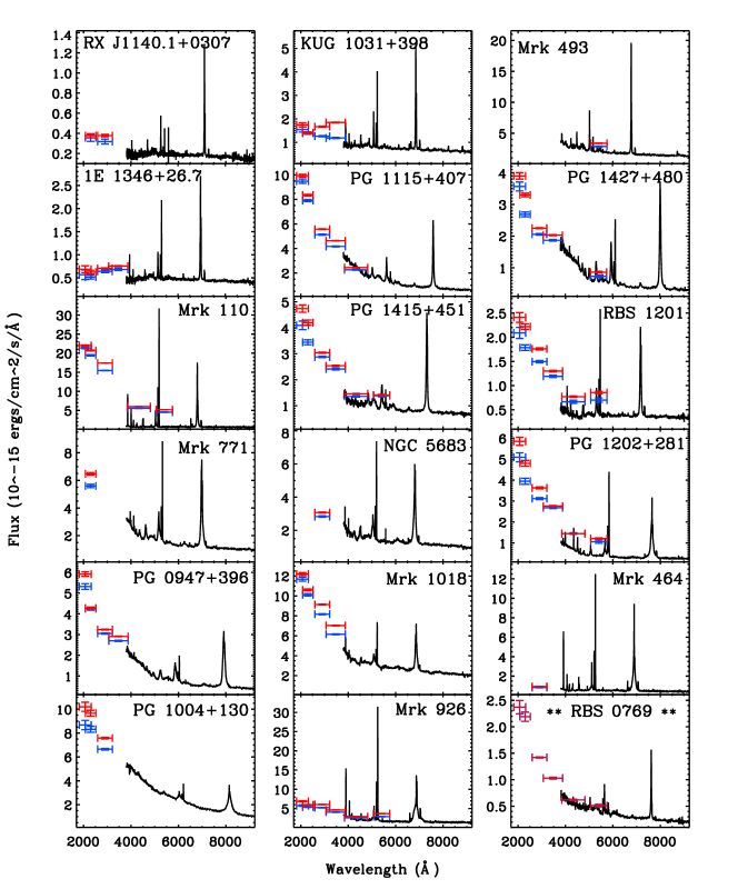
Figure 1: The aperture effect correction results for 17 extended sources in the sample. The point like source RBS 0769 (the last figure marked by **) is also shown for comparison. We over-plot OM data points on to the SDSS spectrum. Red OM points are data obtained directly from the OM PPS files. Blue OM points are the corresponding data after applying a smaller 6″aperture to all OM filters, and applying appropriate OM corrections to the flux eg. deadtime correction, coincidence loss correction and OM time sensitivity degradation correction.

2.3 Characteristics of the Sample

The sample selection procedure described above ensures that every source in our AGN sample has both high quality optical and X-ray spectra. In addition, a large fraction of the sample have simultaneous optical/UV photometric points from the OM monitor. Such high quality data enables accurate spectral fitting. In the optical band our sample is selected to have low reddening, since if present this would significantly modify the intrinsic continuum as well as the optical emission lines. This requirement reduces the complexity and uncertainty in our modeling of the intrinsic continuum, and also increases the overall quality of H$\beta$ and H$\alpha$ line profiles useful for estimating the black hole masses. Furthermore, low reddening is essential in the UV band. The inclusion of OM-UV photometric data observed simultaneously with the X-ray spectra provides a reliable link between these bands. This helps to reduce fitting uncertainty of the SED resulting from optical and X-ray variability. Besides, all sources are well constrained in the 2-10 keV band, which is directly associated with the compact emitting region of the AGN. Our exclusion of objects with evidence of a warm absorber means that the 2-10 keV spectral index is likely to be intrinsic rather than hardened by absorption in the soft X-ray region.

In summary, compared with previous AGN samples used for broadband SED modelling, the spectrally ‘cleaner’ nature of our sample should make the reconstructed broadband SEDs more reliable. Consequently, the parameters derived from the broadband spectral fitting should be more accurate. This may reveal new and potentially important broadband correlations, which we will discuss in detail in paper II.

2.4 Additional Data

The 51 Type 1 AGNs all have SDSS survey-quality spectra (flagged as “sciencePrimary” in SDSS catalog), including 3 objects that have multiple SDSS spectra (i.e. NVSS J030639, 1RXS J111007 and Mrk1018). In such cases we adopt the SDSS spectrum which connects most smoothly with the OM data.

For each object, we used all available EPIC X-ray spectra (i.e. pn, MOS1 and MOS2) for the broadband SED modeling, unless the spectrum had few counts and low S/N. We also searched through the XMM-OM SUSS catalog for all data in the OM bands (i.e. V, B, U, UVW2, UVM2 and UVW1), which are observed simultaneously with the corresponding EPIC spectrum. Of our 51 sources, we have 14 sources with SDSS optical spectra and XMM EPIC X-ray spectra, and 37 sources which in addition to this also have XMM-OM photometry.

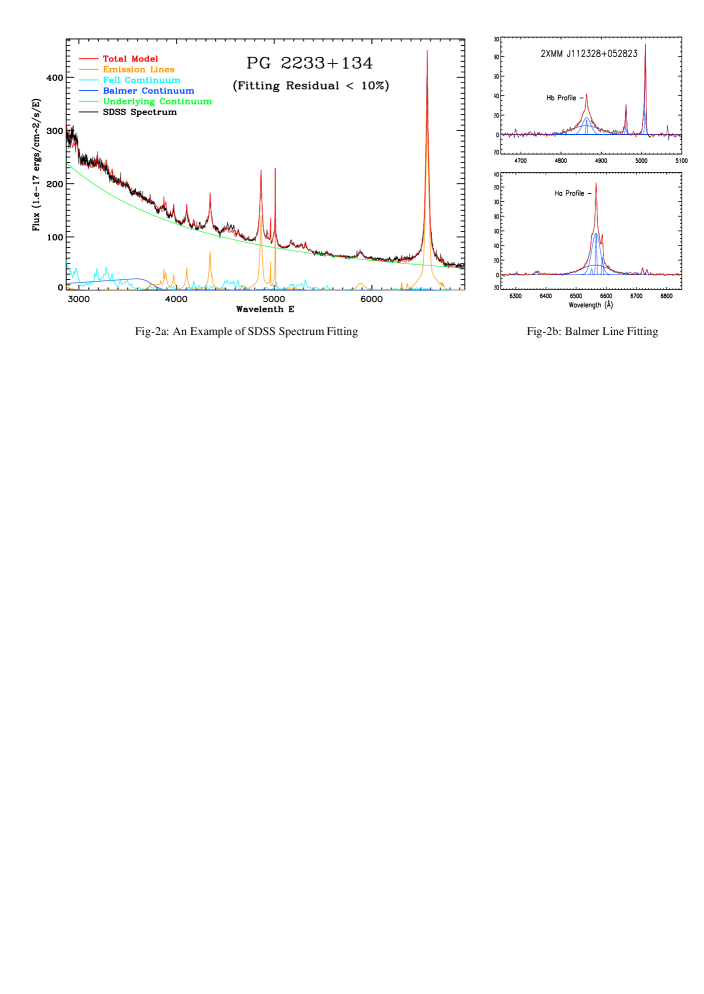
Figure 2: An example of results from SDSS spectrum fitting. The left panel shows a good fit for PG 2233+234. The black line is the observed spectrum, the red line is the total model spectrum. The green line represents the observed underlying continuum. The Balmer continuum (blue), FeII emission (light blue) and other strong emission lines (orange) are shown underneath. The right panel shows an example of detailed line profile fitting to the FeII subtracted region around the H$\beta$ (upper) and H$\alpha$ lines (lower) including H$\alpha$, H$\beta$, [OIII] $\lambda$5007/4959 doublets, [NII] $\lambda$6585/6548 doublets, Li $\lambda$6708, [SII] $\lambda$6717/6733 doublets, [OI] $\lambda$6300/6363 doublets. In our profile fitting, three Gaussian components are used for H$\beta$ and H$\alpha$, two components for [OIII] $\lambda$5007, and one Gaussian for all other lines. The various Gaussian profiles are shown in blue, the total model is shown in red.

2.5 OM Data Corrections and Aperture Effects

In the procedure of combining the SDSS spectra and OM data points, we identified that in some objects there is a clear discrepancy between these two data sets. The OM points often appear higher on the spectral plots (brigher) than is consistent from a smooth extrapolation of the SDSS spectral shape. In fewer cases this discrepancy appears in the opposite sense, with the OM points apparently too low (fainter), see Figure 1 for some examples). This discrepancy may arise for several reasons, including a simple aperture effect. Compared to 3″ diameter for the SDSS spectroscopy fibres, the OM monitor has a much larger aperture, i.e. 12″ and 35″ diameter for the OM optical and OM UV filters respectively (Antonio Talavera.OMCal Team 2009). If the host galaxy is sufficiently extended, e.g. in the case of RE J1034+396, the larger aperture of the OM would include more host galaxy emission than that in the SDSS spectrum (see also section 5.3.1 for other possible reasons to account for this discrepancy). To investigate the aperture issue in more detail, we performed the following tests:
(1) We examined the combined SDSS and OM data plots, searching for those objects with excess OM flux compared with that expected from the extrapolated SDSS spectrum. We identified 27 such cases out of the 51 sources;
(2) Within this sample of 27 sources, we checked the catalog flag for an extended source in each OM filter. We noted those flagged as an extended source in at least one OM filter. This yielded 13 sources out of the 27.
(3) We also extracted the SDSS CCD images for all 51 objects and visually checked whether they appeared extended. As a result, we included another 4 objects for which their SDSS CCD images show that their host galaxy is extended beyond the 3″diameter of the SDSS aperture. Either they were not flagged as extended sources in any OM filter, or they did not have any OM optical data. For these 17 objects, an aperture effect could at least be partially responsible for an excess flux in the OM data.
(4) For these 17 objects we downloaded all available OM image files. In each OM image, we applied a 6″ diameter aperture from which to extract the flux. We used the same sized aperture placed on a blank region of sky close to the object, to estimate the background. The quoted PSF FWHM of the OM for the different filters are: V(1.35″), B(1.39″) , U(1.55″), UVW1(2.0″), UVM2(1.8″), UVW2(1.98″). Thus in all cases 6″ is at least 3$\times$PSF FWHM. So this aperture includes effectively all optical flux for a point source, and more than 90% that from a UV point source detected by the OM.

Before subtracting the background flux from the source+background flux, we performed three count rate calibrations, according the method described in the OM instrument document. The first is the deadtime correction, required because for a small fraction of the exposure time the CCD is in readout mode, and so cannot record events. The second calibration is for coincidence losses, which occur when more than one photon arrives on the CCD at the same location and within the same frame time, so results in under counting. The third calibration is for the OM time sensitivity degradation correction. We performed these calibrations, according to the algorithms set out in the OM instrument document, separately for the background and source+background count rates. We then subtracted the background count rate from the source+background count rate to obtain the corrected source count rate.

Figure 1 shows the OM data points before and after correction for aperture effects for the 17 objects. The reduced OM aperture does improve the alignment between the OM points and SDSS spectrum. This correction not only lowers the OM flux, but also changes the continuum shape defined by the OM points. Although choice of an aperture smaller than 6″ will lower the OM fluxes by a larger factor, it will also introduce uncertainties and systematics caused by the PSF. Therefore we compromise by adopting a 6″ diameter aperture. In our subsequent SED modeling we use the aperture corrected OM data.

3 Optical Spectral Modeling: The Emission Lines

Our optical spectral modeling employs linked $H\alpha$ and $H\beta$ profile fitting and the complete optical spectral fitting. We wrote the code in IDL (Interactive Data Language) v6.2, to perform all the optical spectral fitting. The ‘MPFITEXPR’ program from the Markwardt IDL Library is incorporated within our code to perform the Levenberg-Marquardt least-squares algorithm used to obtain the best-fit parameters. The SDSS spectra (stored in SDSS spSpec files) were extracted directly from the SDSS DR7 data archive and analyzed in IDL using our code. A detailed description of our spectral modeling procedures is presented in the following subsections.

3.1 Profile Fitting of the H$\alpha$, H$\beta$ and [OIII]$\lambda$5007 Emission Lines

Based on current AGN emission line models, there are thought to be stratified regions emitting different lines. These regions are divided somewhat arbitrarily into a narrow line region (NLR), a broad line region (BLR) and possibly an intermediate line region (ILR, e.g. Grupe et al. 1999; Hu et al. 2008; Mei, Yuan & Dong 2009; Zhu, Zhang & Tang 2009). Following previous studies, we use several separate Gaussian profiles representing each of these emitting regions to model the Balmer line profiles.

The H$\alpha$ and H$\beta$ line profiles each pose distinct difficulties for the spectral analysis. In the case of the $H\beta$ line, the permitted FeII emission features (which are often strong in NLS1s) and broad HeII 4686 line blended with the $H\beta$ line, which can affect the determination of the underlying continuum and hence the $H\beta$ line profile. For the $H\alpha$ line, there is the problem of blending with the [NII] $\lambda$6584,6548 doublet, improper subtraction of which may distort $H\alpha$’s intrinsic profile. Our approach, therefore, is to fit $H\alpha$ and $H\beta$ simultaneously using the same multi Gaussian components. The assumed similarity between the intrinsic profiles of these two Balmer lines assists in deblending from other nearby emission lines, and should yield a more robust deconvolution for the separate components of their profile.

3.2 The FeII Problem

We use the theoretical FeII model templates of Verner et al. (2009). These include 830 energy levels and 344,035 transitions between 2000Å and 12000 Å, totaling 1059 emission lines. The predicted FeII emission depends on physical conditions such as microturbulence velocity and hardness of the radiation field, but we use the template which best matches the observed spectrum of I ZW 1 (Boroson & Green 1992, Véron-Cetty et al. 2004) i.e. the one with $n_{H}=10^{11}~{}cm^{-3}$, $v_{turb}=30~{}kms^{-1}$, $F_{ionizing}=20.5~{}cm^{-2}s^{-1}$. Detailed modelling of high signal-to-noise spectra shows that the FeII emission is often complex, with four major line systems in the case of 1 Zw 1, (one broad line system, two narrow high-excitation systems and one low-excitation system Véron-Cetty et al. 2004; Zhou et al. 2006; Mei, Yuan & Dong 2009). However, for simplicity we will assume only one velocity structure and convolve this template with a single Lorentzian profile.

We fit this to the actual FeII emission line features between 5100 Å and 5600 Å (no other strong emission lines lie in this wavelength range) of the de-redshifted SDSS spectra, leaving the FWHM of the Lorentzian and the normalization of the FeII as free parameters. The resulting best-fit FeII model to this restricted wavelength range, was then extrapolated and subtracted from the entire SDSS spectrum. A major benefit from subtracting the FeII features is that the profiles of the [OIII] $\lambda$5007 lines no longer have apparent red-wings. This is particularly important for the NLS1s, where the FeII emission is often strong. After subtracting FeII, we used either 2 or 3 Gaussian components (depending on the profile complexity) to fit the [OIII] $\lambda$5007 line.

3.3 Deconvolution of the Balmer Lines

After fitting the [OIII] $\lambda$5007 line, we start to fit the H$\alpha$ and H$\beta$ line profiles simultaneously. Following previous studies we consider a simplified picture in which the Balmer lines have three principal components, namely a narrow component (from the NLR), an intermediate component (from a transition region ILR between the NLR and BLR or from the inner edge of dusty torus (Zhu, Zhang & Tang 2009)), and a broad component (from the BLR). The intermediate and broad components are both represented by a Gaussian profile, whereas the narrow component is assumed to be similar to that of [OIII] $\lambda$5007. Since we do not know whether or not the Balmer decrements are the same in these different emitting zones, the relative strengths of different line components were not fixed, but their FWHM and relative velocity were both kept the same. The [OIII] $\lambda$4959 line was set at $1/3$ that of [OIII] $\lambda$5007 from atomic physics. The [NII] $\lambda$6584,6548 line doublet were also fixed to the [OIII] $\lambda$5007 line profile. For simplicity, the [SII] $\lambda$6733,6717 doublet, [OI] $\lambda$6300,6363 doublet and Li 6708 were all fitted with a single Gaussian profile separately, because they are all relatively weak lines and do not severely blend with Balmer lines.

In order to separate the narrow component of the Balmer lines from the other components as accurately as possible, particularly for NLS1s and some broad line objects which lack clear narrow line profiles, we applied the following four different fitting methods:
1. The profile of the narrow component is held the same as the entire [OIII] $\lambda$5007 profile; and the normalization of each component in the $H\alpha$ and $H\beta$ lines are left as free parameters;
2. Only the central narrow component of the [OIII] $\lambda$5007 profile is used to define the profile of the Balmer narrow component, and of the [NII] $\lambda$6585,6550 doublet; the normalization of each component in the $H\alpha$ and $H\beta$ lines are free parameters;
3. The shape of the narrow component is held the same as the entire [OIII] $\lambda$5007 profile, and also the normalization of the $H\beta$ line narrow component is set to be 10% of [OIII] $\lambda$5007, this ratio being an average for the NLR in typical Seyfert 1s (Osterbrock & Pogge 1985; Leighly 1999); all other components have their normalizations as free parameters;
4. All conditions are the same as in method 3, except that the Balmer line narrow component and the [NII] $\lambda$6584,6548 doublet adopt the central narrow Gaussian component of the [OIII] $\lambda$5007 line.

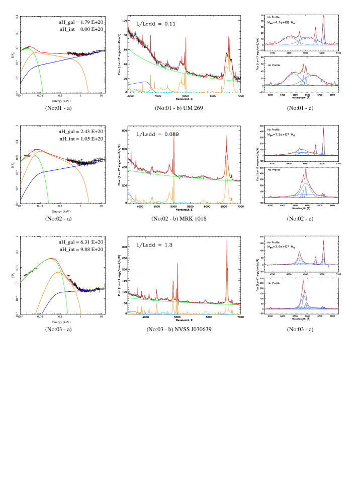
Figure 13: The spectral fitting results. Object order follows all other tables in this paper as increasing RA and DEC. 1. Broadband SED fitting plot (panel-a): X-ray data has been rebinned for each object. Green solid line is the pure accretion disc component peaking at optical/UV region, orange line is Comptonisation component producing soft X-ray excess below 2 keV, blue line is the hard X-ray Comptonisation component dominating 2-10 keV spectrum, and red is the total broadband SED model. 2. SDSS spectrum fitting plot (panel-b): only the fitted spectrum below 7000Å is plotted. Green solid line is the best-fit underlying continuum from accretion disc. Orange line shows all best-fit emission lines, including the results from detailed Balmer line fitting in panel-c. FeII emission is plotted as light blue, while Balmer continuum being dark blue. The total best-fit model with reddening is drawn in red solid line. 3. Balmer emission line fitting plot(panel-c): spectral ranges containing H$\alpha$ and H$\beta$ profiles are plotted separately, with blue lines showing individual line components and red line showing the whole best-fit model. These are also the corresponding zoom-in plots of nearby regions of H$\alpha$ and H$\beta$ in panel-b. The given black hole mass is the broadband SED best-fit value, see Section 5 for detailed descriptions.

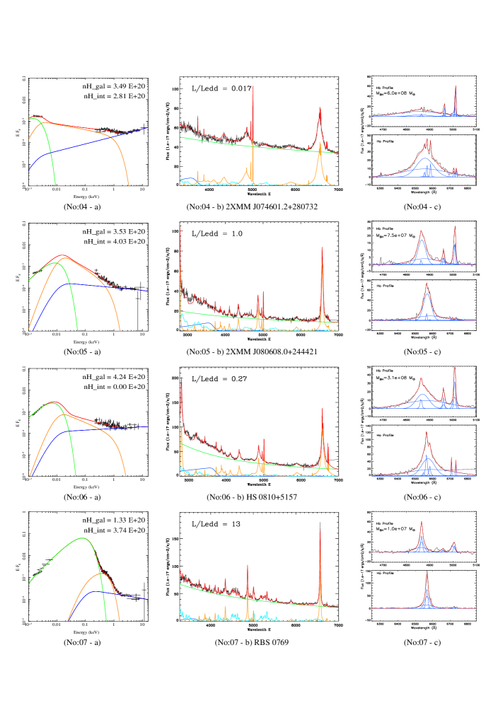
Figure 13: continued

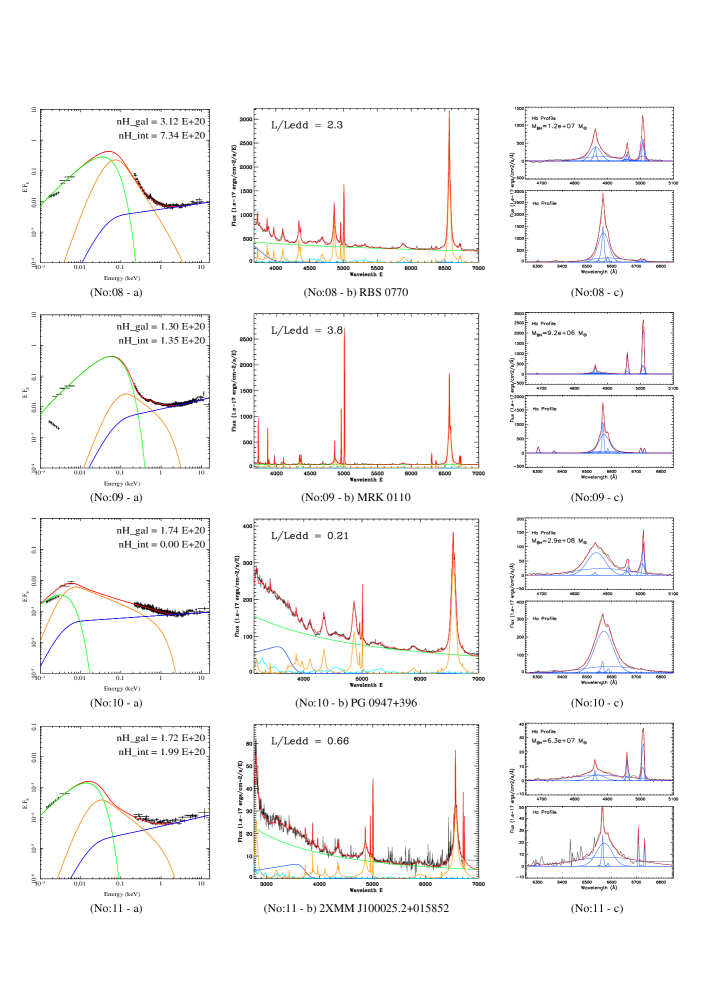
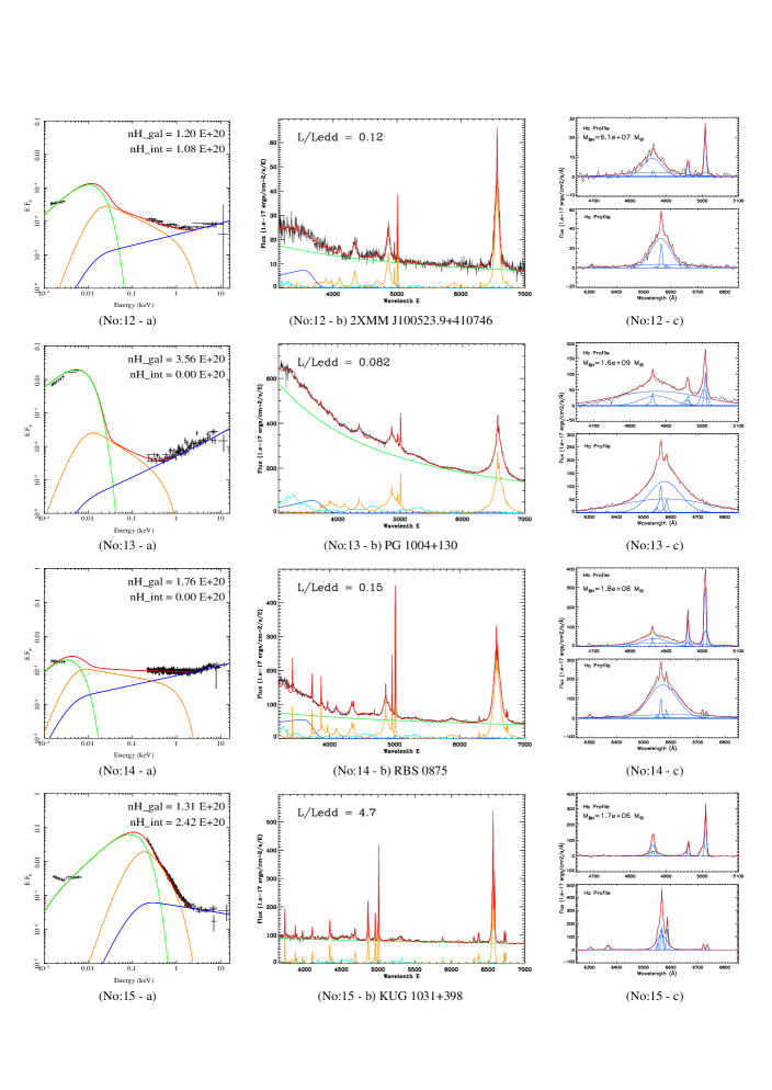
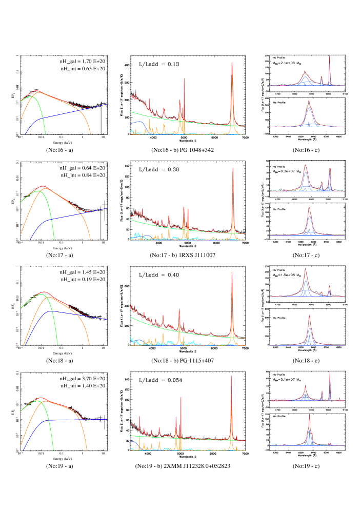
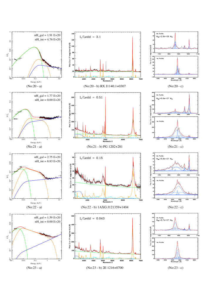
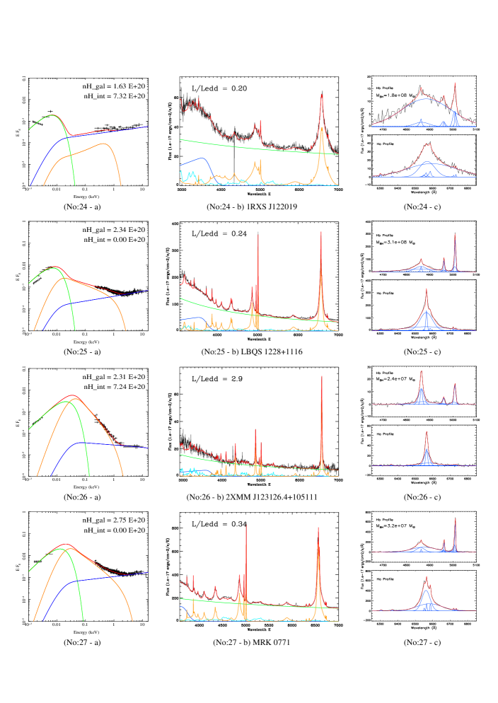
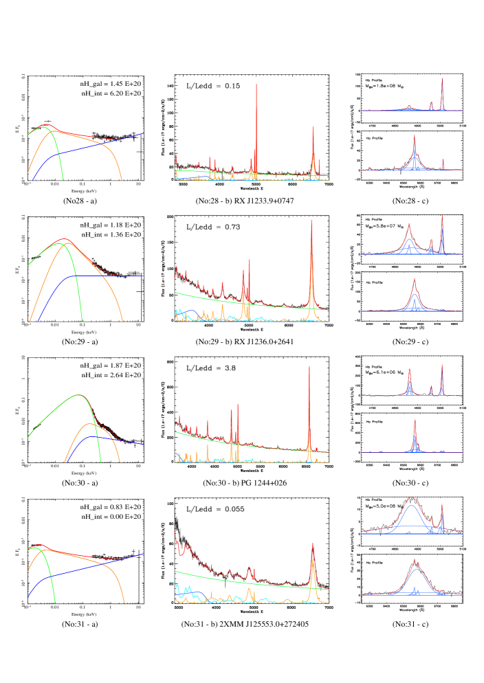
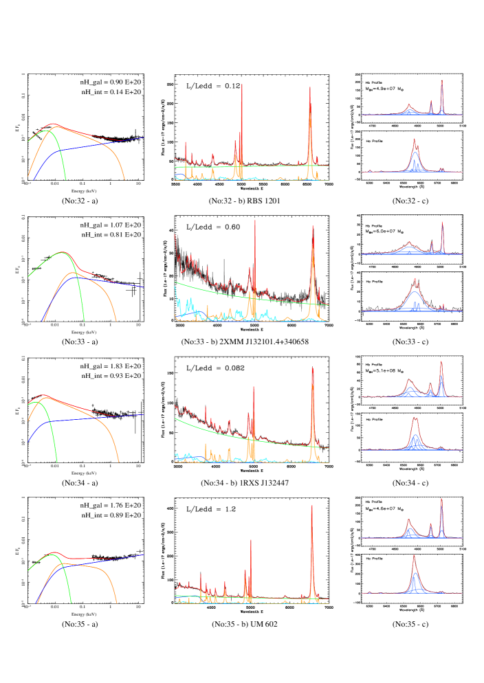
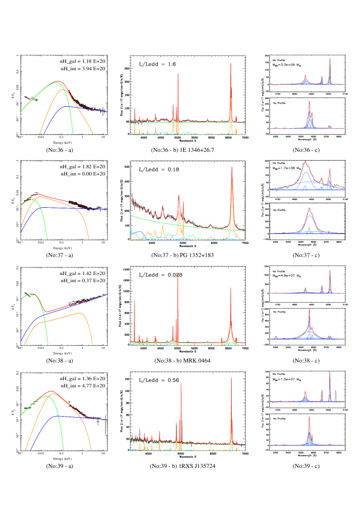
Figure 13: continued

Figure 13: continued

Figure 13: continued

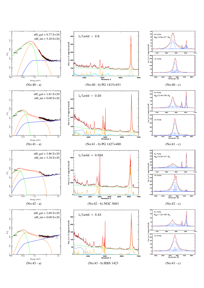
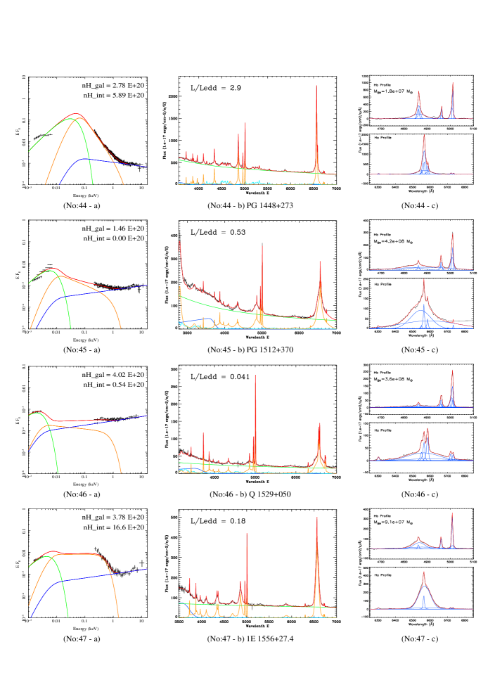
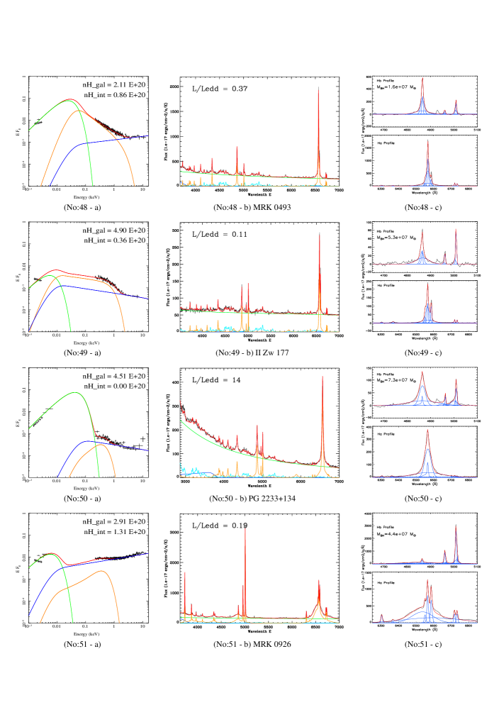
Figure 13: continued

We applied each of the above fitting methods to every object in our sample, and then compared the results. For those objects with clear narrow components to their Balmer lines, we used the best fitting result from method 1 and 2. For the other objects whose narrow components were not clearly defined or even visible, we adopted method 3 and method 4, unless method 1 or 2 gave much better fitting results. Figure 2 right panel shows an example of our fitting. Results for the whole sample are shown in Figure 13.

After obtaining the best-fit parameters, we used the intermediate and broad components to reconstruct the narrow-line subtracted $H\beta$ line profile, and then measured the FWHM from this model. The rationale for using this method, instead of directly measuring the FWHM of the $H\beta$ line from the data, is because for low signal/noise line profiles direct measurement of FWHM can lead to large uncertainties, whereas our profile models are not prone to localized noise in the data. The H$\beta$ FWHM measurements for each of the 51 sources, after de-convolving using the instrumental resolution of 69 $kms^{-1}$, are listed in Table 3.

4 Optical Spectral Modeling

In order to obtain the underlying continuum, we must model the entire SDSS spectrum so that we can remove all the emission lines as well as the Balmer continuum and host galaxy contribution. As we are now concerned with the broad continuum shape, we choose to refit the FeII spectrum across the entire SDSS range, rather than restricting the fit to the H$\alpha$ and H$\beta$ line regions as discussed in the previous section.

Figure 2 shows an illustrative example of our optical spectral fitting, and the results for each of the 51 sources are presented in Figure 13. In the following subsections we give further details of the components that make up these modeled spectra.

4.1 Emission Lines Including FeII

We use the models for [OIII], $H\alpha$ and $H\beta$ as derived above. We add to this a series of higher order Balmer lines: from 5$\rightarrow$2 ($H\gamma$) to 15$\rightarrow$2. We fix the line profile of these to that of $H\beta$ up to 9$\rightarrow$2, then simply use a single Lorentzian profile for the rest weak higher order Balmer lines. We fix the line ratios for each Balmer line using the values in Osterbrock (1989), Table 4.2, with $T_{e}$ between 10,000 K and 20,000 K. We similarly use a single Lorentizan to model the series of Helium lines (HeI 3187, HeI 3889, HeI 4471, HeI 5876, HeII 3204, HeII 4686) and some other emission lines (MgII 2798, [NeIII] $\lambda$3346,4326, [OII] $\lambda$3727,3730, [OI] $\lambda$6302,6366, [NII] $\lambda$6548,6584, Li 6708, [SII] $\lambda$6717,6733).

We use the same model for the FeII emission as described in Section 3.1. However we now fit this to the entire SDSS wavelength range, rather than restricting the fit to 5100–5600 Å.

4.2 The Balmer Continuum

Another potentially significant contribution at shorter wavelengths is from the Balmer continuum. Canfield & Puetter (1981) and Kwan & Krolik (1981) predicted the optical depth at the Balmer continuum edge to be less than 1, we use Equation 1 to model the Balmer continuum under the assumptions of the optically thin case and a single-temperature electron population (also see Grandi 1982; Wills et al. 1985).

$$F_{v}^{BC}=F_{v}^{BE}e^{-h(v-v_{BE})/(kT_{e})}~{}~{}~{}(v\geqslant v_{BE})$$ (1)

where $F_{v}^{BE}$ is the flux at Balmer edge, $v_{BE}$ corresponds to the Balmer edge frequency at 3646Å. $T_{e}$ is the electron temperature. $h$ is the Planck’s constant, $k$ is the Boltzmann’s constant. This Balmer continuum equation is then convolved with a Gaussian profile to represent the real Balmer bump in SDSS spectra.

There are several parameters that may slightly modify or significantly change the shape of the Balmer continuum. It is already seen that the electron temperature $T_{e}$ appearing in Equation 1 and the optical depth can both change the Balmer continuum shape, but there are additional important factors. Any intrinsic velocity dispersion will Doppler broaden all the Hydrogen emission features. Therefore a better description of the Balmer continuum can be obtained by convolving Equation 1 with a Gaussian profile, whose FWHM is determined by the line width of $H\beta$ (or other broad lines), as shown by Equation 2, where G(x) represents a Gaussian profile with a specific FWHM.

$$F_{\lambda}^{BC}=F_{\lambda}^{BE}e^{hc/({\lambda}_{BE}kT_{e})}{\int}_{0}^{+\infty}e^{-hc/({\lambda}kT_{e})}G({\lambda}_{1}-\lambda)d{\lambda}_{1}$$ (2)

Figure 3 shows how the Balmer continuum’s shape depends on the electron temperature and velocity broadening in Equation 2. The electron temperature modifies the decrease in the Balmer continuum towards shorter wavelengths, but has little effect on the broadening of (Balmer Photo-recombination) BPR edge. On the contrary, velocity broadening mainly affects the shape of the BPR edge, but the emission longward of 3646Å is still very weak compared to the emission blueward of the BPR edge, i.e. the BPR edge is still sharp.

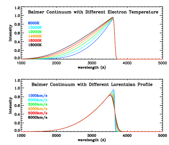
Figure 3: The Balmer continuum models of Grandi (1982). The upper panel shows the dependence of the model on the electron temperature. The lower panel shows the dependence of the model on the FWHM of the convolved Lorentzian profile.

We initially applied Equation 2 to fit the Balmer continuum bump below 4000Å in the SDSS spectra. We assumed the velocity profile for the convolution was a Gaussian with its FWHM determined from the $H\beta$ line profile, and the wavelength of the position of the BPR edge was taken as the laboratory wavelength of 3646Å. However, this model did not provide an acceptable fit, for example see the model shown by the blue line in Figure 4. It appears that the observed spectrum requires a model with either a more extended wing redward of the BPR edge, or a BPR edge that shifts to longer wavelength than 3646Å. However, additional velocity broadening should affect both the Balmer continuum and Balmer emission lines equally, as they are produced from the same material, although the multiple components present in the line make this difficult to constrain.

One way the wavelength of the edge may be shifted without affecting the lines is via density (collisional, or Stark) broadening (e.g. Pigarov et al. 1998). Multiple collisions disturb the outer energy levels, leading to an effective $n_{max}$ for the highest bound level $\ll\infty$, i.e. lowering the effective ionization potential. We set the edge position and the FWHM as free parameters, and let the observed spectral shape determine their best fit values. The red line shown in Figure 4 represents a good fit, obtained with FWHM of 6000 $kms^{-1}$ and the BPR edge wavelength of 3746 Å, which implies $n_{max}\sim 12$. The theoretical $n_{max}$ can be determined by the plasma density $N_{e}$ and temperature $T_{e}$ as $n_{max}=2\times 10^{4}(T_{e}/N_{e})^{1/4}$ (Mihalas 1978), so for a typical temperature of $10^{4-5}K$, the required density is $7\times 10^{16-17}$ cm^-3. Such high density is not generally associated with the BLR clouds, and may give support to models where the low ionization BLR is from the illuminated accretion disc (e.g. Collin-Souffrin & Dumont 1990). However, any reliable estimation of the density would require more accurate subtraction of other optical components such as the FeII line blends and many other non-hydrogen emission lines, which is not the focus of this paper. Nonetheless, this remains an interesting problem which is worthy of further study.

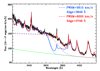
Figure 4: An expanded view of the region around the BPR edge in PG 1427+480. The blue and dashed lines represent the Balmer continuum model superposed on the underlying disc continuum (green solid line) using standard parameters (blue dash), and also a set of best fit parameters (red dash line). The red and blue solid lines are models of the total optical spectrum, including the corresponding Balmer continuum components and plus other components described in the text. The observed spectrum is shown in black.

Yet another issue in modeling the Balmer continuum is how to quantify the the total intensity of this continuum component, especially when there is limited spectral coverage bellow 4000Å, which makes it difficult to define the overall shape. The theoretical flux ratio between the Balmer continuum and the $H\beta$ line under case B conditions can be expressed by Equation 3 (Wills et al. 1985),

$$I(Bac)/I(H\beta)=3.95~{}T_{4}^{0.4}$$ (3)

but other theoretical calculations of photonionization models show that by varying the Balmer optical depth, electron temperature and electron number density, this can result in very different values of I(Bac)/I(H$\beta$). For example, Canfield & Puetter (1981)’s calculation resulted in a I(Bac)/H$\alpha$ range of 0.05$\sim$10, Kwan & Krolik (1981) suggested I(Bac)/I(H$\beta$)=1.6$\sim$15, and other theoretical work also confirmed a large range in flux ratios (Puetter & Levan 1982; Kwan 1984; Hubbard & Puetter 1985). The observed ranges in I(Bac)/I(H$\beta$) are also large. Canfield & Puetter (1981) showed an observed range of 0.5$\sim$3 for I(Bac)/I(H$\alpha$). Wills et al. (1985) observed 9 intermediate redshift QSOs whose I(Bac)/I(H$\beta$) ranges from 4.65$\sim$9.5. Thus we were unable to constrain the intensity of the whole Balmer continuum by using a standard flux ratio fixed to the other Balmer emission lines. As a result, we must rely on the shape of the observed Balmer bump, and then adopt the model’s best fit parameters.

However, this limitation in defining the Balmer bump introduces uncertainties in modeling the underlying continuum, because over-subtraction of the Balmer bump will depress the slope of the remaining underlying continuum, and vice-versa. In the course of the broadband SED fitting described in section 5, we found that the temperature of accretion disc (determined by black hole mass) is sensitive to the slope of optical continuum, unless the continuum slope is in the opposite sense to that of the accretion disc model and thus can not be fitted, or there are OM points providing stronger constraints. We also found that a flatter optical continuum may lead to a lower best-fit black hole mass, although this also depends on other factors. Therefore, the subtraction of the Balmer continuum can have an impact on the modeling of broadband SED and the best-fit black hole mass. The influence of this depends on the relative importance of other SED restrictions. This is the reason why the Balmer continuum must be carefully modeled and subtracted.

4.3 The Intrinsic Underlying Continuum

Our basic assumption is that the residual optical spectrum, after subtraction of the Balmer continuum, FeII emission and other emission lines mentioned previously, arises mainly from the accretion disc emission. As a reasonable approximation over a limited wavelength range we use a powerlaw of the following form to fit the underlying continuum,

$$F(\lambda)=C_{1}{\cdot}({\lambda}/5100\AA)^{-C_{2}}$$ (4)

The powerlaw approximation for the optical underlying disc continuum is also widely adopted in previous and recent AGN optical spectral studies. (e.g. Grandi 1982; Tsuzuki et al. 2006; Zhou et al. 2006; Landt et al. 2011).

We model the dust reddening using the Seaton (1979)’s 1100Å to 10000Å reddening curve, and we apply this to the overall model, i.e. emission lines, Balmer continuum and the disc continuum. There are also other reddening curves available such as Fitzpatrick (1986) for the Large Magellanic Cloud, Prévot et al. (1984) and Bouchet et al. (1985) for the Small Magellanic Cloud and Calzetti et al. (2000) for starburst galaxies, but over the wavelength range of 2500Å to 10000Å, the difference between these reddening curves is small, except for Calzetti et al. (2000)’s curve which is appropriate for starburst galaxies, and is thus not applicable for our AGN sample.

4.4 The Host Galaxy Contribution

Many previous studies on AGN’s optical/infrared spectra have adopted a powerlaw as a reasonable approximation for the accretion disc continuum blueward of 1$\mu$m (e.g. Mei, Yuan & Dong 2009; Bian & Huang 2010), but these studies also needed to include additional contributions from the host galaxy and emission from the dusty torus to account for the extra continuum emission at long wavelengths of the optical spectrum (e.g. Kinney et al. 1996; Mannucci et al. 2001; Landt et al. 2011). In our work we have also identified an inconsistency between the 3000Å$\sim$8000Å spectral shape and a single powerlaw shape (i.e. the flat optical spectrum problem discussed in Section 5.3.2). The blue end of the optical spectrum, presumed to arise from a standard accretion disc, often shows a steeper spectral slope than the red end.

However, in our sample we found evidences suggesting only a weak if any, contribution from the host galaxy. For example, the optical spectra of our sample do not show the strong curvature characteristic of the presence of a stellar component in a host galaxy. Furthermore, the good quality optical spectra do not exhibit stellar absorption features (see Section 5.3.2 and Figure 5). In fact the 3$\arcsec$ diameter fibre used to obtain the SDSS spectra also helps to reduce the contribution of stellar emission from a host galaxy, particularly for nearby sources in our sample such as KUG 1031+398. These evidences argues against the possibility that the red optical continuum is primarily dominated by host galaxy emission. In fact, it is possible that the observed additional component arises due to emission from the outer regions of a standard accretion disc (e.g. Soria & Puchnarewicz 2002; Collin & Kawaguchi 2004; Hao et al. 2010). The existence of such an additional red optical continuum component reduces the consistency of a powerlaw fit to the optical spectra.

4.5 The Optical Spectrum Fitting

Our optical spectral fitting is performed only for data blueward of 7000Å. The choice to truncate the model at 7000Å is made for several reasons. We wish to include H$\alpha$ line in the spectral fitting range, and the broad wing of H$\alpha$ profile sometimes extend to $\sim$7000Å (e.g. PG 1352+183, RBS 1423, Mrk 926). There are some objects whose SDSS spectra extend only to $\sim$6700Å (e.g. 2XMM J080608.0+244421, HS 0810+5157, 2XMM J100025.2+015852). The choice of 7000Å, rather than a longer wavelength, is to maintain consistency of optical spectral fitting for the whole sample. The final reason concerns an aspect of the powerlaw fitting. We found that in some objects (e.g. PG 1115+407, LBQS 1228+1116, PG1352+183), a flat slope power-law under predicts the observed emission at $\sim$7000Å. Therefore, if we include longer wavelengths than 7000Å, our powerlaw fitting for the standard accretion disc continuum towards the blue optical spectra would be biased by other continuum emission at these longer wavelengths, and so affect the broadband SED fitting. Consequently, we chose to truncate our optical spectral fitting at 7000Å.

However, we still cannot be sure that the underlying continuum is totally free from other non-disc continuum components. So after completing the fitting procedure, we then checked the spectral fitting status within two narrow wavebands, i.e. 4400Å - 4800Å and 5100Å - 5600Å. Emission features if present in these two wavebands are mainly from FeII emission, and the underlying continua of these two wavebands should be totally dominated by the accretion disc emission. Assuming that the FeII emission lines within these two wavebands have similar relative intensity ratios as in the FeII template described in Section 3.2, the best-fit underlying powerlaw plus FeII emission model should have good fitting status in both of these two wavebands. In general, the best-fit model derived from the full optical spectrum fit also gives reasonably good fitting status in both of these two narrow wavebands. However, in some cases the model over-predicted the flux in 5100Å - 5600Å but under-predicted the flux in 4400Å - 4800Å, so that we should slightly increase the slope of powerlaw to produce better spectral fitting in these two wavebands. We adopted these parameter values in preference to those directly from the full spectrum fit, as they should be more immune to problems such as host galaxy or hot dust contamination.

Table 2: Broadband SED Fitting Parameters, and Model Outputs (L_bol, f_d, f_c, f_p). ID: object number, the same as Table 1; N_H,gal and N_H,int: the fixed galactic and free intrinsic neutral hydrogen column densities in 10²⁰ $cm^{-2}$; $\Gamma_{pow}$: the powerlaw component’s slope in the SED fitting, (*) denotes the objects whose powerlaw slopes hit the uplimit of 2.2 and were fixed there; Fpl: the fraction of powerlaw component in the total reprocessed disc emission; R_cor: corona (truncation) radius in unit of Gravitational radii (r_g) within which all disc emission is reprocessed into the Comptonisation and powerlaw components; T_e: temperature of the Compton up-scattering electron population; Tau: optical depth of the Comptonisation component; log(M_BH): the best-fit black hole mass; log($\dot{M}$): total mass accretion rate; L_bol: bolometric luminosity integrated from 0.001 keV to 100 keV; f_d, f_c, f_p: luminosity fractions of disc emission, soft Comptonisation and hard X-ray Compotonisation components in the bolometric luminosity; $\chi^{2}$: the reduced $\chi^{2}$ of the broadband SED fitting.

ID	NH,gal	NH,int	$\Gamma_{pow}$	Fpl	Rcor	Te	Tau	log(MBH)	log($\dot{M}$)	Lbol	fd	fc	fp	$\chi^{2}$
	$\times{\it 10}^{\it 20}$	$\times{\it 10}^{\it 20}$			$r_{g}$	keV		M☉	$g$ $s^{-1}$	${\it 10}^{\it 44}$				reduced
1	1.79	0.00	1.71	0.69	100.	0.262	17.2	8.61	26.06	58.9	0.19	0.25	0.56	1.00
2	2.43	1.06	1.77	0.39	100.	0.226	15.7	7.85	25.21	8.28	0.19	0.49	0.32	0.97
3	6.31	9.88	1.91	0.25	11.9	0.108	20.0	7.41	25.92	42.9	0.87	0.10	0.03	1.57
4	3.49	2.81	1.66	0.50	100.	0.312	15.4	8.78	25.41	13.3	0.19	0.41	0.40	1.15
5	3.53	4.03	2.12	0.36	54.9	0.205	14.9	7.87	26.28	98.4	0.32	0.44	0.24	1.10
6	4.24	0.00	1.93	0.46	23.9	0.347	12.6	8.50	26.33	111	0.59	0.22	0.19	1.02
7	1.33	3.74	2.20∗	0.29	8.37	0.137	40.3	7.00	26.53	175	0.26	0.53	0.21	1.20
8	3.12	7.35	1.82	0.15	24.1	1.380	3.44	7.09	25.85	36.6	0.58	0.35	0.06	1.39
9	1.30	1.36	1.71	0.71	12.9	0.360	11.1	6.96	25.94	45.0	0.84	0.05	0.11	17.2
10	1.74	0.00	1.91	0.32	100.	0.295	13.8	8.47	26.20	81.5	0.19	0.55	0.26	1.72
11	1.72	2.00	1.71	0.49	20.2	0.449	9.23	7.80	26.02	53.8	0.65	0.18	0.17	1.01
12	1.20	1.08	1.68	0.48	20.6	0.402	11.4	7.79	25.27	9.46	0.65	0.18	0.17	1.20
13	3.56	0.00	1.37	0.87	10.9	0.146	17.9	9.20	26.52	170	0.90	0.01	0.09	3.12
14	1.76	0.00	1.72	0.71	100.	0.294	16.0	8.24	25.82	33.6	0.19	0.23	0.58	1.07
15	1.31	2.43	2.20∗	0.09	14.2	0.214	12.3	6.23	25.31	10.4	0.80	0.18	0.02	2.27
16	1.70	0.65	1.72	0.31	100.	0.327	13.0	8.33	25.85	36.2	0.19	0.56	0.25	1.44
17	0.65	0.85	1.74	0.14	48.7	0.326	11.4	7.97	25.85	36.5	0.35	0.56	0.09	1.08
18	1.45	0.19	2.20∗	0.24	29.5	0.254	13.6	8.17	26.18	76.9	0.51	0.37	0.12	1.37
19	3.70	1.41	1.98	0.19	45.8	0.142	21.5	7.71	24.85	3.61	0.37	0.52	0.12	1.10
20	1.91	4.77	2.20∗	0.36	9.63	0.210	16.8	6.46	25.36	11.9	0.94	0.04	0.02	1.39
21	1.77	0.00	1.79	0.75	22.7	0.206	19.6	7.98	26.09	63.4	0.61	0.10	0.29	3.59
22	2.75	8.84	1.86	0.21	50.5	0.108	25.1	7.84	25.42	13.5	0.34	0.52	0.14	1.09
23	1.59	0.00	1.41	0.45	86.9	0.626	9.59	7.99	25.02	5.40	0.22	0.43	0.35	0.99
24	1.63	0.00	1.82	0.94	32.2	0.182	32.2	8.26	25.96	46.5	0.48	0.03	0.49	2.13
25	2.34	0.00	1.79	0.40	25.7	0.351	12.9	8.49	26.26	94.2	0.56	0.27	0.17	1.83
26	2.31	7.25	2.10	0.03	33.8	0.310	9.69	7.37	26.23	87.7	0.46	0.52	0.02	1.14
27	2.75	0.00	1.85	0.22	37.6	0.554	8.29	7.50	25.44	14.2	0.43	0.45	0.12	1.12
28	1.45	0.00	1.69	0.60	71.3	0.353	13.7	8.24	25.81	33.0	0.26	0.30	0.45	1.26
29	1.18	1.36	2.00	0.12	30.9	0.389	8.85	7.76	26.03	55.1	0.49	0.45	0.06	1.24
30	1.87	2.64	2.20∗	0.36	9.67	0.234	16.9	6.79	25.77	30.3	0.94	0.04	0.02	1.03
31	0.84	0.00	1.68	0.54	100.	0.404	12.9	8.70	25.84	35.9	0.19	0.37	0.43	0.99
32	0.90	0.14	1.80	0.44	100.	0.388	12.2	7.69	25.15	7.30	0.19	0.46	0.35	1.66
33	1.07	0.82	2.18	0.57	15.0	0.226	15.6	7.78	25.96	47.3	0.78	0.10	0.13	1.15
34	1.83	0.93	1.90	0.33	100.	0.252	14.8	8.71	26.03	55.1	0.19	0.54	0.26	1.11
35	1.76	0.90	1.80	0.83	100.	0.202	20.4	7.67	26.13	69.8	0.19	0.14	0.67	1.05
36	1.18	3.94	2.18	0.22	16.2	2.000	2.71	6.52	25.13	6.90	0.75	0.20	0.05	1.81
37	1.82	0.00	2.04	0.38	100.	0.219	17.2	8.23	25.88	39.3	0.19	0.50	0.31	1.33
38	1.42	0.37	1.58	0.97	100.	0.251	25.0	7.69	24.54	1.80	0.19	0.02	0.79	1.28
39	1.36	4.77	2.10	0.11	40.6	0.281	11.4	7.01	25.17	7.57	0.40	0.53	0.07	1.90
40	0.77	5.21	2.05	0.06	24.0	0.930	4.28	7.41	26.26	93.6	0.59	0.39	0.02	2.27
41	1.81	0.00	1.90	0.39	28.9	0.298	14.0	8.39	26.10	65.2	0.52	0.30	0.19	1.63
42	2.86	3.29	1.84	0.41	100.	0.083	31.3	7.74	24.68	2.45	0.19	0.47	0.33	1.01
43	2.69	0.00	1.71	0.58	55.8	0.406	11.9	8.07	26.10	64.7	0.31	0.29	0.40	1.29
44	2.78	5.90	2.17	0.04	27.6	0.501	6.71	7.26	26.13	68.6	0.53	0.45	0.02	2.33
45	1.46	0.00	1.82	0.49	41.0	0.286	14.1	8.62	26.75	290	0.40	0.30	0.30	2.42
46	4.02	0.55	1.81	0.81	100.	0.207	20.3	8.56	25.58	19.4	0.19	0.15	0.66	1.12
47	3.78	16.69	1.82	0.25	100.	0.115	29.8	7.96	25.62	21.5	0.19	0.61	0.20	0.99
48	2.11	0.87	1.85	0.19	18.1	0.525	8.61	7.19	25.16	7.40	0.70	0.24	0.06	1.19
49	4.90	0.36	2.20∗	0.33	72.5	0.211	19.6	7.73	25.15	7.33	0.25	0.50	0.25	1.15
50	4.51	0.00	2.20∗	0.80	7.88	0.131	48.5	7.86	27.42	1350	0.98	0.00	0.01	1.39
51	2.91	1.53	1.79	0.95	100.	0.112	45.2	7.65	25.32	10.8	0.19	0.04	0.77	1.38

Table 3: Broadband SED Key Parameters. ID: object number, the same as Table 1; $\Gamma_{2-10keV}$: the slope of the single powerlaw fitted to 2-10 keV spectrum. L_2-10keV: 2-10 keV luminosity (in 10⁴⁴ erg s^-1); $\kappa_{2-10keV}$: the 2-10keV bolometric correction coefficient; $\lambda$L_2500Å: the monochromatic luminosity at 2500Å (in 10⁴³ erg s^-1); $\nu$L_2keV: the monochromatic luminosity at 2keV (in 10⁴³ erg s^-1); $\alpha_{ox}$: the optical X-ray spectral index; $\lambda$L₅₁₀₀: the monochromatic luminosity at 5100Å (in 10⁴⁴ erg s^-1); $\kappa_{5100}$: the 5100Å bolometric correction coefficient; FWHM_Hβ: the narrow component subtracted H$\beta$ FWHM; L_bol/L_Edd: the Eddington Ratio.

ID	$\Gamma_{2-10keV}$	L2-10keV	$\kappa_{2-10keV}$	$\lambda$L2500Å	$\nu$L2keV	$\alpha_{ox}$	$\lambda$L5100	$\kappa_{5100}$	FWHMHβ	Lbol/LEdd
		$\times{\it 10}^{\it 44}$		$\times{\it 10}^{\it 43}$	$\times{\it 10}^{\it 43}$		$\times{\it 10}^{\it 44}$		km s-1
1	1.69$\pm$0.06	4.941	11.9	81.3	25.6	1.19	8.15	7.24	13000	0.11
2	1.67$\pm$0.10	0.469	17.7	18.4	2.47	1.33	0.791	10.5	6220	0.089
3	1.77$\pm$0.07	0.289	149	41.0	1.91	1.51	1.35	31.7	2310	1.3
4	1.80$\pm$0.11	0.567	23.6	12.8	3.15	1.23	1.91	6.98	10800	0.017
5	2.10$\pm$0.22	2.284	43.2	134	12.9	1.39	5.48	18.0	2720	1.0
6	1.93$\pm$0.18	4.855	22.9	290	27.6	1.39	14.8	7.52	5430	0.27
7	2.39$\pm$0.22	0.267	657	61.3	2.43	1.54	1.95	89.6	1980	13
8	1.84$\pm$0.04	0.418	87.7	23.5	2.89	1.35	0.539	68.1	2840	2.3
9	1.76$\pm$0.01	0.839	53.8	22.7	5.35	1.24	0.113	399	3030	3.8
10	1.92$\pm$0.05	3.532	23.1	205	23.1	1.36	7.59	10.8	4810	0.21
11	1.71$\pm$0.11	1.811	29.8	78.9	9.03	1.36	3.75	14.4	5640	0.66
12	1.68$\pm$0.23	0.502	18.9	21.2	1.57	1.43	1.04	9.12	4390	0.12
13	1.37$\pm$0.12	0.751	227	790	2.99	1.93	42.6	4.00	10800	0.082
14	1.69$\pm$0.04	3.189	10.6	50.2	17.0	1.18	3.91	8.60	7060	0.15
15	2.35$\pm$0.12	0.042	251	2.89	0.353	1.35	0.204	51.1	988	4.7
16	1.78$\pm$0.07	1.502	24.2	90.8	8.24	1.40	4.26	8.53	3560	0.13
17	1.80$\pm$0.20	0.779	46.9	71.7	3.62	1.50	3.31	11.1	2250	0.30
18	2.23$\pm$0.08	1.254	61.5	157	9.67	1.46	6.11	12.6	2310	0.40
19	1.98$\pm$0.18	0.084	43.1	8.59	0.497	1.47	0.443	8.19	2000	0.054
20	2.34$\pm$0.12	0.053	224	4.44	0.476	1.37	0.215	55.4	774	3.1
21	1.70$\pm$0.04	3.856	16.5	109	20.5	1.28	2.22	28.6	6090	0.51
22	1.70$\pm$0.09	0.396	34.1	27.3	2.17	1.42	0.983	13.8	7050	0.15
23	1.80$\pm$0.19	0.145	37.5	11.5	0.907	1.42	0.708	7.66	1980	0.043
24	1.83$\pm$0.18	4.735	9.84	106	25.1	1.24	6.64	7.01	13900	0.20
25	1.88$\pm$0.03	3.054	30.9	249	20.0	1.42	8.44	11.2	4980	0.24
26	2.09$\pm$0.25	0.362	243	63.3	2.60	1.53	2.04	43.2	1720	2.9
27	1.94$\pm$0.04	0.277	51.5	20.3	2.51	1.35	0.988	14.4	4310	0.34
28	1.71$\pm$0.14	2.951	11.2	63.6	13.2	1.26	4.80	6.91	4240	0.15
29	2.00$\pm$0.12	0.726	76.0	76.3	4.75	1.46	3.25	17.0	3560	0.73
30	2.46$\pm$0.09	0.146	207	13.4	1.28	1.39	0.452	67.2	954	3.8
31	1.69$\pm$0.14	2.420	14.9	53.6	11.9	1.25	6.49	5.54	6810	0.055
32	1.88$\pm$0.03	0.464	15.8	13.7	2.97	1.26	0.512	14.3	3100	0.12
33	2.14$\pm$0.21	1.157	41.0	69.7	7.55	1.37	4.03	11.8	5690	0.60
34	1.90$\pm$0.14	2.489	22.2	140	13.5	1.39	10.8	5.13	3310	0.082
35	1.76$\pm$0.07	3.918	17.9	67.5	51.5	1.04	3.59	19.5	2790	1.2
36	2.20$\pm$0.08	0.091	76.3	3.31	0.651	1.27	0.244	28.4	1890	1.6
37	1.95$\pm$0.08	1.768	22.3	88.8	12.3	1.33	5.39	7.30	3960	0.18
38	1.55$\pm$0.09	0.175	10.3	1.89	0.768	1.15	0.197	9.16	6630	0.028
39	2.17$\pm$0.20	0.079	96.5	6.89	0.737	1.37	0.233	32.6	991	0.56
40	2.02$\pm$0.06	0.468	200	70.0	3.54	1.50	2.05	45.7	2790	2.8
41	1.94$\pm$0.05	2.444	26.7	167	15.8	1.39	6.26	10.4	2610	0.20
42	1.76$\pm$0.11	0.158	15.5	4.92	0.804	1.30	0.265	9.28	4920	0.034
43	1.74$\pm$0.07	4.524	14.3	109	25.7	1.24	4.36	14.9	4550	0.43
44	2.25$\pm$0.05	0.236	292	45.5	2.13	1.51	2.36	29.2	1070	2.9
45	1.82$\pm$0.06	17.502	16.6	645	98.4	1.31	30.4	9.58	10900	0.53
46	1.81$\pm$0.12	2.175	8.93	19.0	10.4	1.10	2.97	6.55	9930	0.041
47	1.45$\pm$0.25	0.868	24.9	36.6	4.39	1.35	0.931	23.2	4100	0.18
48	2.03$\pm$0.11	0.101	73.2	8.71	0.734	1.41	0.278	26.7	1190	0.37
49	2.40$\pm$0.22	0.200	36.8	14.5	1.69	1.36	0.719	10.2	1340	0.11
50	2.41$\pm$0.18	3.299	411	860	27.3	1.57	29.5	46.0	2200	14
51	1.67$\pm$0.03	1.659	6.50	12.5	8.30	1.07	0.624	17.3	11100	0.19

5 The Broadband SED Modeling

5.1 Data Preparation

For each object we extracted the original data files (ODFs) and the pipeline products (PPS) from XMM-Newton Science Archive (XSA) . In the following data reduction process, tasks from XMM-Newton Science Analysis System (SAS) v7.1.0 were used. First, EPCHAIN/EMCHAIN tasks were used to extract events unless the events files had already been extracted for each exposure by PPS. Then ESPFILT task was used to define background Good Time Intervals (GTIs) that are free from flares. In each available EPIC image, a 45″radius circle was used to extract the source region, and an annulus centered on the source with inner and outer radii of 60″and 120″was used to define the background region. For other sources listed in the region files of PPS that are included in these regions, these were subtracted using the default radii generated by PPS, which scaled with the source brightness. Then the GIT filter, source and background region filters were applied to the corresponding events files to produce a set of source and background events files. We only accepted photons with quality flag =0 and pattern 0$\sim$4. The EPATPLOT task was then used to check for pile-up effects. When pile-up was detected, an annulus with inner and outer radii of 12″and 45″was used instead of the previous 45″radius circle to define the source region. Then source events files were reproduced using the new source region filter. Source and background spectra were extracted from these events files for each available EPIC exposure. Tasks RMFGEN/ARFGEN were used to produce response matrices and auxiliary files for the source spectra. These final spectra were grouped with a minimum of 25 counts per bin using the GRPPHA v3.0.1 tool for spectral fitting in Xspec v11.3.2. To prepare the OM data, the om_filter_default.pi file and all response files for the V,B,U, UVW1, UVM2, UVW2 filters were downloaded from the OM response file directory in HEASARC Archive. We then checked the OM source list file for each object to see if there were any available OM count rates. Each count rate and its associated error were entered into the om_filter_default.pi file and then combined with the response file of the corresponding OM filter, again by using the GRPPHA tool to produce OM data that could be used in Xspec.

Finally, the XMM-Newton EPIC spectra are combined with the aperture corrected OM photometric points, and the optical continuum points produced from the optical underlying continuum (obtained from the full optical spectrum fitting) using FLX2XSP tool. From these data we constructed a broadband nuclear SED of each AGN. There is a ubiquitous data gap in the far UV region which is due to photo-electric absorption by Galactic gas. Unfortunately, in most cases of low-redshift AGN, their intrinsic SED also peaks in this very UV region, and so this unobservable energy band often conceals a large portion of the bolometric luminosity. In order to account for this, and to estimate the bolometric luminosity, we fit the X-ray and UV/optical continua all together using a new broadband SED model (Done et al. 2011, Xspec model: optxagn). We then calculate the bolometric luminosity by summing up the integrated emission using the best-fit parameters obtained for each continuum component.

5.2 The Broadband SED Model

A standard interpretation of the broadband SED is that the emission is dominated by a multi-temperature accretion disc component which peaks in the UV (e.g. Gierliński et al. 1999, Xspec model: diskpn). This produces the seed photons for Compton up-scattering by a hot, optically thin electron population within a corona situated above the disc, resulting in a power law component above 2 keV (e.g. Haardt & Maraschi 1991; Zdziarski, Poutanen & Johnson 2000, Xspec model: bknpl). However, the X-ray data clearly show that there is yet another component which rises below 1 keV in almost all high mass accretion rate AGNs. The ubiquity of this component can be seen, for example, in the compilation of AGN SEDs presented in Middleton, Done & Gierliński (2007), and one of the strongest cases is the NLS1 RE J1034+396 (Casebeer, Leighly & Baron 2006; Middleton et al. 2009) and RX J0136.9-3510 (Jin et al. 2009). The origin of this so-called soft X-ray excess is still unclear (e.g. Gierliński & Done 2004; Crummy et al. 2006; Turner et al. 2007; Miller, Turner & Reeves 2008), and so some previous broadband SED modeling studies have explicitly excluded data below 1 keV. An obvious consequence is that in such studies a soft excess component cannot influence the models, so making it possible to fit the data using just a disc and (broken) power law continuum (VF07; Vasudevan & Fabian 2009). However, in our current study we include all of the data, and so we require a self-consistent model which incorporates this soft component.

Whatever the true origin of the soft X-ray excess, the simplest model which can phenomenologically fit its shape is the optically thick, low temperature thermal Comptonisation model (compTT). But the observed data are used to constrain the three separate components, discpn + compTT + bknpl, which is generally problematic given the gap in spectral coverage between the UV and soft X-ray regions caused by interstellar absorption. So instead, we combine these three components together using a local model in xspec, assuming that they are all ultimately powered by gravitational energy released in accretion. A complete description of this model can be found in the Xspec website⁵ and is also given in Done et al. (2011). It is in essence a faster version of the models recently applied to black hole binary spectra observed close to their Eddington limit (Done & Kubota 2006) and to the (possibly super Eddington) Ultra-Luminous X-ray sources (Gladstone, Roberts & Done 2009; Middleton & Done 2010), thus this model is more appropriate for fitting a medium sized sample of objects. A comprehensive comparison with the model of Done & Kubota (2006) is given in Done et al. (2011). To make this paper self contained we give a brief synopsis of the model. We assume that the gravitational energy released in the disc at each radius is emitted as a blackbody only down to a given radius, $R_{corona}$. Below this radius, we further assume that the energy can no longer be completely thermalised, and is distributed between the soft excess component and the high energy tail. Thus the model includes all three components which are known to contribute to AGN SED in a self consistent way. As such it represents an improvement on the fits in VF07 in several respects, by including the soft excess and by requiring energy conservation, and it improves on Done & Kubota (2006) by including the power law tail.

In our SED fitting, the optical/UV data constrains the mass accretion rate through the outer disc, provided we have an estimate of the black hole mass. We constrain this by our analysis of the $H\beta$ emission line profile. The main difference from previous studies based on non-reverberation samples is that we do not directly use the FWHM of the H$\beta$ profile to derive the black hole mass. Rather, we use the FWHM of the intermediate and broad line component determined from the emission line fitting results presented in Section 3.1. These are then used in Equation 5 (Woo & Urry 2002 and references therein) to derive the black hole mass limits required for the SED fitting:

$$M_{BH}=4.817{\times}[{{{\lambda}L_{\lambda}(5100{\AA})}\over{10^{44}ergs^{-1}}}]^{0.7}{FWHM}^{2}$$ (5)

where $L_{\lambda}$(5100Å) is measured directly from the SDSS spectra. The rms difference between the black hole masses from this equation and from the reverberation mapping study is $\sim$0.5 dex. Thus we also adopted any best-fit values that fell below the original lower limit (which was set by FWHM of the intermediate component) by less than 0.5 dex. With this method, the best-fit black hole mass found by SED fitting is always consistent with the prediction from the H$\beta$ profile. Section 6.5 discusses the differences between the best-fit black hole masses and those estimated using other methods.

Once the black hole mass is constrained, the optical data then sets the mass accretion rate $\dot{M}$, and hence the total energy available is determined by the accretion efficiency. We assume a stress-free (Novikov-Thorne) emissivity for a Schwarzschild black hole, i.e. an overall efficiency of 0.057 for $R_{in}=6R_{g}$. Thus the total luminosity of the soft excess and power law is $0.057\dot{M}c^{2}(1-R_{in}/R_{corona})$. This constrains the model in the unobservable EUV region, with the input free parameter $R_{corona}$ setting the model output of the luminosity ratio between the standard disc emission and Comptonisation components. The upper limit of $R_{corona}$ is set to be 100 $R_{g}$, which corresponds to 81% released accretion disc energy. This upper limit is based on the requirement that the seed photons should be up-scattered (Done et al. 2011). We assume that both the Comptonisation components scatter seed photons from the accretion disc with temperature corresponding to $R_{corona}$. The other model input parameters are; the temperature ($kT_{e}$) and optical depth ($\tau$) of the soft Comptonisation component which are determined by the shape of the soft X-ray excess, the spectral index ($\Gamma$) of the hard X-ray Comptonisation that produces the 2-10 keV power law, with electron temperature fixed at 100 keV. The model output $f_{pl}$ represents the fraction of the non-thermalised accretion energy (i.e. given by the luminosity originating from the region of $R_{corona}$ to $R_{in}$), which is emitted in the hard X-ray Comptonisation.

We also included two sets of corrections for attenuation (reddening-wabs), to account for the line of sight Galactic absorption and for the absorption intrinsic to each source, the latter is redshifted (zred and zwabs in Xspec). The Galactic HI column density is fixed at the value taken from Kalberla et al. (2005), but the intrinsic HI column density is left as a free parameter. The standard dust to gas conversion formula of E(B-V)=$1.7\times 10^{-22}N_{H}$ (Bessell 1991) is used for both Galactic and intrinsic reddening. We set the initial value of the powerlaw photon index to be that of the photon index in 2-10 keV energy band, but it can vary during the fitting process. However, we set an upper limit of 2.2 for the powerlaw photon index, not only because the photon index is $<$ 2.2 for the majority of Type 1 AGNs (Middleton, Done & Gierliński 2007), but also because otherwise the much higher signal-to-noise in the soft excess in some observed spectra can artificially steepen the hard X-ray powerlaw and result in unphyiscal best-fit models.

All free parameters used in the broadband SED fitting are listed in Table 2. For completeness, we also explicitly calculate the fraction of the total luminosity carried by each component of the model (i.e. disc: $f_{d}$; soft Comptonization: $f_{c}$; hard X-ray Comptonization: $f_{p}$) from the model fit parameters R_cor and F_pl (see Table 2) . Table 3 lists the important characteristic parameters. The main uncertainty in these parameters, especially the black hole mass, is dominated by other systematic uncertainties introduced by the observational data, model assumptions (e.g. the assumption of a non-spinning black hole and the inclination dependence of the disc emission) and the analysis methods involved. Therefore the parameter fitting uncertainties which are often less than 10%, are not significant in comparison, and thus are not listed. The statistical properties of these parameters are discussed in section 6.

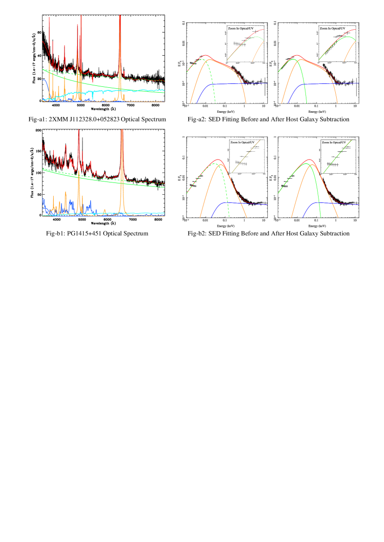
Figure 5: A comparison between the results of two subtractions of host galaxy contribution. 2XMM J112328+052823 (Fig-a1 and Fig-a2) shows an underlying continuum that more closely resembles a disc continuum (solid green line in Fig-a1) after modelling and subtracting the host galaxy contribution (light blue spectrum in Fig-a1). The left panel of Fig-a2 shows the original broadband SED fitting without subtracting the host galaxy contribution. The dashed green line shows the modelled accretion disc emission in the best-fit SED. The inserted panel shows a magnification of the fit in the optical/UV region, where a big discrepancy exists between the SDSS data and best-fit SED model. The right panel of Fig-a2 is the new SED fit using the new underlying disc continuum (shown as solid green line in Fig-a1) after subtracting the host galaxy contribution. The new fit is improved in the optical region compared with the previous results in the left panel of Fig-a2. In contrast to the above example, PG 1415+451 (Fig-b1 and Fig-b2) has little host galaxy contribution in the SDSS optical spectrum (see the light blue component in Fig-b1), and its broadband SED fitting in the optical region remains poor regardless of the amount of host galaxy subtraction applied (see the two panels in Fig-b2). The spectral template for Elliptical galaxies in Kinney et al. (1996) was used in both cases since their host galaxies both have elliptical morphologies in SDSS image.

5.3 Problems in The SED Fitting

We further discuss two problems we encountered during the fitting procedure in the following subsections. The first problem is the discrepancy between the OM and SDSS continuum points (mentioned in Section 2.5). The second problem is that of the observed flat optical continuum, whose shape cannot be accounted for in our SED model (mentioned in Section 4.4).

5.3.1 The discrepancy between the OM photometry and the SDSS continuum

There remains a significant discrepancy between many of the OM and SDSS continuum points, even after applying the aperture correction discussed in Section 2.2 (see Figure 13). The OM points often appear above (brighter) the extrapolation of the SDSS continuum to the OM wavelengths. We identify three possible reasons for this discrepancy:

(1) Remaining aperture effects: There is an aperture difference between the SDSS fibres (3″diameter) and the OM apertures we used (6″diameter). Clearly the OM points will still include more host galaxy starlight than the SDSS points, and so will appear above the SDSS spectrum.

(2) Contamination from emission lines: The wavelength ranges for each OM filter (over which the effective transmission is greater than 10% of the peak effective transmission) are as follows: UVW2 1805-2454Å, UVM2 1970-2675Å, UVW1 2410-3565Å, U 3030-3890Å, B 3815-4910Å, V 5020-5870Å. We exclude the contribution from strong optical emission lines within the OM U, B, V bandpass (and also the Balmer continuum contribution in U band) by using the best-fit optical underlying continuum which excludes such features from the SDSS spectral fitting. In fact, this was an important initial motivation of the study, i.e. to obtain more accurate estimates of the true underlying continuum rather than simply to use the SDSS ‘ugriz’ photometric data. Inclusion of strong emission lines within these photometric data would result in over-estimation of the optical continuum, and so compromise our aim to study the shape of the optical underlying continuum. This is an important spectral characteristic used to constrain the accretion disc component in the SED fitting (see also the discussion in section 5.1.2). There are some strong emission lines within the UV bandpasses such as Ly$\alpha$, CIV 1549, CIII 1909 and MgII 2798, whose fluxes are not available from SDSS spectrum. Accurate subtraction of these line fluxes for each object would require new UV spectroscopy. We conclude that inclusion of emission line flux within the OM photometric points may account for some of the observed discrepancy.

(3) Intrinsic source variability: AGN are well known to be variable across their SEDs. In general there is a significant time difference between acquistion of the SDSS and OM-UV data, so intrinsic variation may contribute to any observed discrepancy. Mrk 110 is the most extreme example of this phenomena in our sample, as its SDSS spectrum has a very large discrepancy compared with the OM data. The recent paper by Landt et al. (2011) gives another set of optical spectra for Mrk 110, which is more consistent with our best-fit model. It shows that the inclusion of OM data is useful to help identify cases such as this. As an additional test for variability, we assembled all available GALEX data for our sample. We find that 43 objects in our sample have GALEX data. Using a GALEX aperture of 12″, which is limited by the PSF and which is also similar to the UV OM apertures, we compare these values with the SED model. The ratio of the GALEX data and our SED model within the same bandpass differ by less than a factor of 2 for the majority of our sample, and significantly the flux ratio distribution is almost symmetric and is centered close to unity. This suggests that the non-simultaneous OM and SDSS data is not likely to be a major impediment to our modeling.

In effect, these three factors will merge together to produce the observed discrepancy between the SDSS and OM data. Since the combined effects of Point (1) and (2) which will add flux and generally be greater than that caused by optical/UV variability as shown by previous long term reverberation mapping studies (Giveon et al. 1999; Kaspi et al. 2000), we should treat the OM points included in our SED modeling as upper limits when interpreting the results of our modeling. Indeed, the 90% confidence uncertainties in the BH masses derived directly from the Xspec fitting are almost certainly small compared with the systematic errors introduced by the above uncertainties.

5.3.2 The observed flat optical continuum

A related problem in our fitting is about the SDSS continuum shape. For some AGNs, their SDSS continuum data points exhibit a very different spectral slope from that of the SED model. This cannot be reconciled by adjusting the parameters of the accretion disc model, and thus implies the presence of an additional component at longer optical wavelengths, which flattens compared with that predicted by the accretion disc models. One obvious explanation for this flux excess is the contribution from the host galaxy. In late type host galaxies such as elliptical and S0 galaxies, emission from their old stellar populations peaks at near infrared wavelengths. Kinney et al. (1996) combined spectra of quiescent galaxies and constructed an average spectral template for each morphological type, including bulge, elliptical, S0, Sa, Sb, Sc and starburst galaxies. For some objects in our sample with high S/N SDSS spectra which show at least marginal stellar absorption features, we have added the corresponding type of host galaxy spectral template taken from Kinney et al. (1996), into the overall SDSS spectral fitting. This revised underlying continuum in the optical, and was then used in the broadband SED fitting. We are then able to compare it with the original fit, to see how the subtraction of a stellar population template effects the overall SED fitting.

Figure 5 shows two examples. The first is 2XMM J112328.0+052823, in which after subtracting the host galaxy component, the observed optical continuum is closer to the slope of the SED model. However, the results for PG1415+451 in Figure 5 lower panel imply that its host galaxy cannot be the origin of the flat optical spectrum. The reason is that its optical spectrum does not show any strong stellar absorption features. This means that the maximum amount of host galaxy contribution is small, and so and there remains a substantial inconsistency in the slope versus the SED model. In addition to 2XMM J112328.0+052823 above, only Mrk1018 and 2XMM J125553.0+272405 show clear stellar absorption features. Also the 3″diameter fibre excludes much of the host galaxy component at these redshifts. Therefore, on these general grounds we conclude that host galaxy contamination is small for most sources in our sample, and consequently cannot fully account for the observed flat optical continuum. Additional support for this view comes from good correlations between the X-ray components and the red optical continuum, suggesting that this extra optical flux is likely related to the intrinsic activity (e.g. Soria & Puchnarewicz 2002; Collin & Kawaguchi 2004; Hao et al. 2010; Landt et al. 2011).

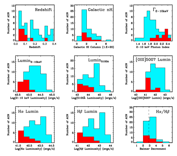
Figure 6: Distributions of our sample for different properties. In each panel the blue areas show the distribution for the whole sample, while the red areas show the distribution for the 12 NLS1s in our sample. We note that the H$\alpha$, H$\beta$ and [OIII] $\lambda$5007 luminosities are based on results of line profile fitting, after subtracting the blends from other nearby emission lines (see Section 3.1). For comparison we also indicate the Balmer decrement value of 2.86, found under case B recombination, as shown by dashed line in the same panel.

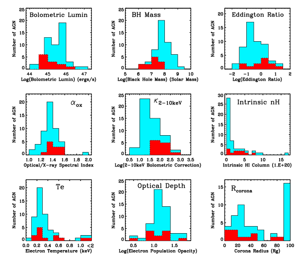
Figure 7: The distribution of model dependent parameters using the same colour coding as in Figure 6. Comments on each distribution are given in Section 6.2.

6 Statistical properties of the sample

Histograms of data on our sample are shown in Figure 6, Figure 8 and Figure 9, including redshift, HI column density, optical and X-ray modeling parameters etc. The red region in the histograms show the distributions for the 12 NLS1s in our sample. It is clear that NLS1s are distinct among the whole sample in several respects.

6.1 General Properties

Figure 6 shows some basic properties of our sample which are not model dependent:
(1). Redshift: the sample’s redshift ranges from 0.031 (Mrk 493) to 0.377 (HS 0810+5157). The NLS1s are found mainly at lower redshifts, with $<z>_{n}=0.12$ compared to the $<z>_{n}=0.19$ for the BLS1s. For comparison we see that the sample of VF07 has a similar redshift range, but it has a lower average redshift of 0.10.
(2). The Galactic nH: the average Galactic nH is $2.25{\times}10^{20}$.
(3). The photon indexes obtained from simple power law fits to the restricted energy range of 2-10 keV. The NLS1s cluster on the higher photon index side, with an average of $2.21{\pm}0.20$, which differs from the sample average of $1.92{\pm}0.25$ and the BLS1s’ average of $1.83{\pm}0.18$. This means that NLS1s tend to have softer X-ray spectra, which is further confirmed in the following section on the mean SEDs.
(4). The X-ray continuum and 2-10 keV luminosity: this distribution shows that NLS1s have lower 2-10 keV luminosities in spite of their steeper slopes. We note that the VF07 sample has a similar distribution, except for their inclusion of three extremely low X-ray luminosity AGN (i.e. NGC4395, NGC3227 and NGC6814), these objects were not included in our sample due to our selection criteria and/or a lack of SDSS spectra.
(5). The optical continuum luminosity at 5100 Å. On average the NLS1 have lower optical luminosities than BLS1.
(6-8). The [OIII] $\lambda$5007, H$\alpha$ and H$\beta$ emission line luminosities. Again the NLS1s have on average lower luminosities than BLS1s.
(9). The Balmer decrement. The average value for the whole sample is 3.14$\pm$0.62, and for NLS1s is 3.05$\pm$0.38. This difference is not statistically significant, but we return to the issue in our next paper (paper II), where we consider the separate components as well as the overall profile.

6.2 Results from The Broadband SED Modeling

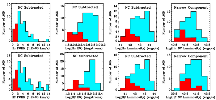
Figure 8: The Balmer line parameter distributions. The first row is for H$\alpha$ and the second is for H$\beta$. We combine the intermediate and broad components in each Balmer line profile to form the total broad line properties, giving values of the FWHM, EW and luminosity. The final panel shows the luminosity distribution of the narrow component for comparison. The distributions for the 12 NLS1s are indicated by the red regions, as in Figure 6.

Figure 7 shows properties derived from the SED fits:
(1). The bolometric luminosity: the distribution range is between $1.8{\times}10^{44}ergs$ $s^{-1}$ (Mrk 464) and $1.4{\times}10^{47}ergs$ $s^{-1}$ (PG 2233+134). There is no clear difference in the distribution of the complete sample and the sub-set of NLS1s. The average luminosity is Log(L_bol)=45.49$\pm$0.55, which is consistent with the value of 45.19$\pm$1.01 found in VF07 sample, except for the three extremely nearby and low luminosity AGNs in VF07.
(2). The black hole mass: using the best-fit black hole masses, the whole sample peaks between $10^{7}M_{\odot}$ and $10^{8}M_{\odot}$. Equation 5 suggests that the black hole mass should depend on both H$\beta$ FWHM and L₅₁₀₀, and the results from our SED fitting suggest that NLS1s with smaller Balmer line FWHM do indeed harbour lower mass black holes. KUG 1034+396 has the lowest black hole mass in our sample. The value of $1.7{\times}10^{6}M_{\odot}$ is consistent with the estimate based on the first firmly detected AGN QPO (quasi periodic oscillation) found in this source (Gierliński et al. 2008). Again we can compare our results with those of VF07 sample. We find that their average black hole mass is 7.89$\pm$0.82, calculated using the M(L₅₁₀₀, FWHM_Hβ) relation. Adopting this same method for our sample, we find a very similar average of 7.99$\pm$0.93. Our best-fit masses have a slightly lower average value of 7.83$\pm$0.64 (also see Section 6.5 for a comparison of different estimates of black hole masses).
(3). The Eddington ratio: the average values are 3.21$\pm$3.07 for NLS1 which display a wide dispersion, and 0.57$\pm$0.50 for BLS1 and 0.93$\pm$0.85 for the whole sample. Of the eight objects whose Eddington ratios are above 1, six are NLS1 galaxies, and the highest value is 14.2 (PG 2233+134). Clearly, NLS1s tend to have larger Eddington ratios. Our Eddington ratio distribution is also similar to that found in the sample of VF07 whose average value is 0.47$\pm$0.44, except that their distribution has a more pronounced peak at $\sim$0.1.
(4). The $\alpha_{ox}$ index, is defined between restframe continuum points at 2500 Å and 2 keV (see Lusso et al. 2010 and references therein). The distribution for NLS1 is peaked at marginally higher values than for BLS1.
(5). The $\kappa_{2-10}$ bolometric correction, is defined as $L_{bol}/L_{2-10}$ (see VF07 and references therein). We find that NLS1s have a significantly higher fraction of their bolometric luminosity emitted as hard X-rays than the BLS1s. Compared with the VF07 sample, both distributions peak at $\kappa_{2-10}$=10$\sim$30, but our sample shows a smoother distribution decreasing as $\kappa_{2-10}$ increases after $\sim$30, and so results in a slightly higher average value of $\kappa_{2-10}$.
(6). The intrinsic nH: This distribution shows that the intrinsic equivalent neutral hydrogen column densities are low for our sample, which is a natural consequence of our initial sample selection criteria. The NLS1s have slightly higher intrinsic absorption than BLS1s, which may imply a slightly higher dust reddening. However the distribution of Balmer decrements shows no significant difference between these two types of AGNs.
(7). The temperature of the Comptonisation component used to describe the soft X-ray excess. This is close to 0.2 keV in all objects, confirming the trend seen in previous studies for this component to exhibit a narrow range of peak energy (Czerny et al. 2003; Gierliński & Done 2004). The distribution peak at this energy is more marked for the BLS1 than for NLS1, although the small number statistics means that this difference cannot be considered as definitive for our sample.
(8). The optical depth of the soft excess Comptonised component. It is clear that this component is always optically thick, with most objects having $\tau{\sim}10-30$. There is no significant difference in temperature or optical depth between the broad and narrow line objects.
(9). There is a difference in the coronal radii distribution between the BLS1s and NLS1s. Corona radius controls the relative amount of power emerging from the accretion disc and the soft X-ray excess/hard tail. There are two peaks in the distribution for the broad line objects, one between 10 and 20 R_g (where $R_{g}=GM/c^{2}$), and the other at 100 R_g (which is set as the upper limit of this parameter in our broadband SED model). By contrast these radii in NLS1 are consistent with just the first peak. At first sight this is surprising, since NLS1 are expected to be those with the strongest soft X-ray excess. However, their similar soft excess temperatures around 0.2 keV suggests that atomic processes may be significant (reflection and/or absorption from partially ionized material), and this may influence our fits. The average coronal radii are 32$\pm$26 R_g for NLS1, 59$\pm$37 R_g for BLS1 and 53$\pm$36 R_g for the whole sample. This supports the conclusion of VF07 that high Eddington ratio AGN have lower coronal fractions compared to those with low Eddington ratios.

6.3 Balmer Line Parameter Distribution

Figure 8 shows further details of the modeled profiles of $H\alpha$ (first row), and $H\beta$ (second row).
(1). The FWHM of the broad emission profile. This is calculated from co-adding the two best fit Gaussian profiles for the broad and intermediate line components, and then using the resultant profile to determine the FWHM. This is equivalent to subtracting the narrow line core from the observed profile and measuring the resultant FWHM.
Note, the NLS1s by definition have H${\alpha}<2000$ km $s^{-1}$.
(2-3). The equivalent widths and line luminosities are again measured using the total broad emission line profile as above. The NLS1s have both lower equivalent widths and line luminosities.
(4). By contrast, there is no pronounced difference between NLS1s and BLS1s in their Balmer narrow line component. This suggests that the narrow line region is less influenced by whatever difference in properties is responsible for the defining difference between NLS1s and BLS1s in the broad line region.

6.4 The Bolometric Luminosities

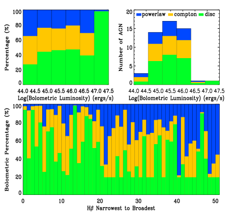
Figure 9: The bolometric luminosity distribution for the different continuum components of the SED, i.e. accretion disc (green), Comptonisation (orange) and hard X-ray Comptonisation (blue). The upper left panel shows the percentage within each luminosity bin for each of these three SED components. The Upper right panel shows the luminosity distribution of the whole sample, with each bin divided into three regions according to the fractional contribution from the different components in that luminosity bin. The lower panel shows how the contribution from each component changes as a function of rank order in H$\beta$ FWHM, after the narrow line component has been removed.

The fraction of the total luminosity contained in each component of the SED model is shown in Figure 9. The upper left panels show these fractions as a function of the bolometric luminosity. It seems that as the bolometric luminosity increases, the disc component slightly increases in importance. However, the total numbers of objects at high luminosities is small, as seen in the upper right panels, where the fraction is multiplied by the number of objects in the bin, so we should be cautious about this finding.

The lower panel shows this fraction for each of the objects ranking from the smallest to biggest $H\beta$ FWHM. Thus low rank objects have the narrowest $H\beta$ (and hence are by definition NLS1s). These also have the lowest black hole masses and highest Eddington ratios. They are more likely to have a smaller fraction of their total luminosity emitted in the soft X-ray excess component, than the BLS1s. This relates to the issue of the coronal radii, see Point (9) of Section 6.2. There are also some BLS1s which have an apparently high fraction of power in their soft X-ray excesses, but they may also have alternative spectral fits including reflection and/or absorption.

We note that in all these plots the lower limit to the disc fraction of $0.19$ results from setting an upper limit of 100 R_g for the coronal radius parameter, as mentioned in Section 5.2

Table 4: The average black hole masses, as shown in Figure 10.

	NLS1	BLS1	ALL
$<$M${}_{BH,IC}>$	6.58$\pm$0.49	8.09$\pm$0.56	7.73$\pm$0.84
$<$M${}_{BH,BC}>$	7.72$\pm$0.49	9.05$\pm$0.55	8.74$\pm$0.78
$<$M${}_{BH,IC+BC}>$	6.75$\pm$0.49	8.37$\pm$0.65	7.99$\pm$0.93
$<$M${}_{BH,\sigma}>$	6.57$\pm$0.46	7.89$\pm$0.47	7.58$\pm$0.73
$<$M${}_{BH,FIT}>$	7.11$\pm$0.54	8.05$\pm$0.48	7.83$\pm$0.64
$<$M${}_{BH,RP}>$	7.42$\pm$0.39	8.44$\pm$0.53	8.20$\pm$0.66

6.5 The Black Hole Mass

The black hole mass is one of the key parameters used in our SED fitting, and it largely determines the continuum shape in the optical/UV region. The masses derived from reverberation mapping are considered to be the most accurate, but the total number of objects which have been studied using this technique is still relatively small (e.g. Peterson et al. 2004; Denney et al. 2010; Bentz et al. 2010). In the absence of reverberation mapping, the empirical relation between M_BH and H$\beta$ linewidth and L₅₁₀₀ is often used as a proxy to estimate the black hole mass (Peterson et al. 2004). A serious limitation of this method is that it is still not clear which specific measure of the H$\beta$ profile provides the closest association with the velocity dispersion of the gas in the broad line region.

There are various alternative measures of the velocity width used for determining the black hole mass, including the FWHMs of the intermediate component (IC) and the broad component (BC) (e.g. Zhu, Zhang & Tang 2009). One could also use the model independent second momentum (e.g. Peterson et al. 2004; Bian et al. 2008), or more simply the FWHM of the H$\beta$ line after subtracting the narrow component (NC) (e.g. Peterson et al. 2004). The NC subtracted FWHM and the second momentum estimates often lie within the range of values covered by the IC and BC FWHMs, except for some peculiar objects such as those with broad double-peaked profiles, for example UM 269. Given all these uncertainties we decided to adopt the the best-fit black hole mass obtained from the SED model, rather than simply fixing it at a value determined from a specific linewidth measurement. Moreover, it is now suggested that radiation pressure may be important in modifying the black hole mass derived using the relation between M_BH and L₅₁₀₀ and H$\beta$ FWHM, especially for objects with high Eddington ratios such as most NLS1s (e.g. Marconi et al. 2008).

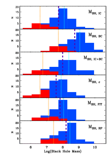
Figure 10: A comparison of various methods used to derive black hole mass. The total distributions are shown with the 12 NLS1s show by the red regions. The purple dashed line indicate the average black hole mass for the whole sample. The orange and cyan dotted lines indicate the average masses of NLS1s and BLS1s, respectively. The average values are listed in Table 4. Values for individual objects are listed in Table 6.

In order to compare our results with those from other studies, we have made various estimates of black hole masses for every source in our sample as follows:
(1) M_BH,IC, M_BH,BC and M_BH,IC+BC are derived using Equation 5 with different H$\beta$ FWHMs obtained from our Balmer line fitting procedure.
(2) M_BH,σ is the black hole mass calculated from the second momentum of the total H$\beta$ line profile (see Peterson et al. (2004) for details of the definition of ‘second momentum’), by using R${}_{BLR}\propto$L${}_{5100}^{0.518}$ and a geometry factor of $f=3.85$. These assumptions are considered to be appropriate when using second momentum as a measure of the velocity dispersion in BLR (Bentz et al. 2006; Collin et al. 2006; Bian et al. 2008).
(3) M_BH,RP is the black hole mass corrected for radiation pressure, using equation (9) in Marconi et al. (2008) with $f=3.1$, $log(g)=7.6$.
We compare the black hole mass distributions obtained from these different methods in Figure 10. The mean values are listed in Table 4.

The M_BH,IC and M_BH,BC represent the two extreme estimates of black hole masses. The M_BH,IC could still be influenced by contamination from a NLR component, especially for NLS1s where deconvolution of the narrow and broad components is very difficult. If there is a residual narrow line component, it will introduce a bias that underestimates black hole masses. Conversely, using M_BH,BC is more likely to bias towards higher black hole masses, due to the presence of low contrast very broad wings often seen in H$\beta$ profiles. We found FWHM_IC+BC/$\sigma_{H\beta}$=1.30$\pm$0.39 for our sample, which is consistent with 1.33$\pm$0.36 found by Bian et al. (2008). This leads to slightly lower values of M_BH,σ than M_BH,IC+BC, but these two methods both give black hole masses between M_BH,IC and M_BH,BC, with M_BH,IC+BC spanning a broader mass range.

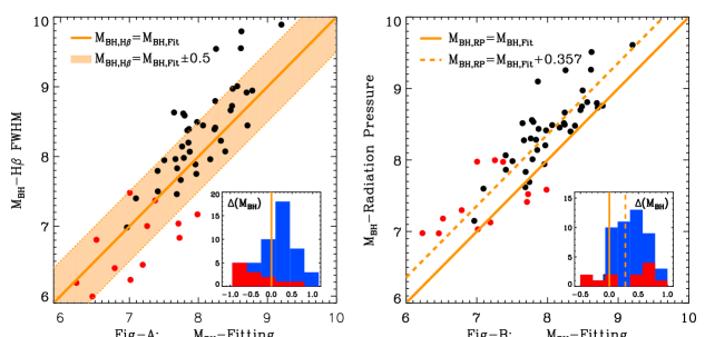
Figure 11: Correlations of best-fit black hole mass (‘M_BH-Fitting’ or ‘M_BH,FIT’) vs. H$\beta$ FWHM determined black hole mass (‘M_BH-H$\beta$ FWHM’ or ‘M_BH,IC+BC’) and vs. radiation pressure corrected black hole mass (‘M_BH-Radiation Pressure’ or ‘M_BH,RP’). Red points represent the 12 NLS1s. The inserted panel in panel-A shows the distribution of the mass difference between M_BH,IC+BC and M_BH,FIT, while the inserted panel in panel-B shows the distribution of the mass difference between M_BH,RP and M_BH,FIT. Red regions highlight the distribution of NLS1s.

Our best-fit SED black hole masses (M_BH,FIT) are also distributed between M_BH,IC and M_BH,BC, with similar average masses as M_BH,IC+BC (a comparison is shown in Figure 11 Panel-A). Note that M_BH,FIT is a free parameter in the SED fitting unless it hits the lower or upper limits set by M_BH,IC and M_BH,BC, which occasionally happened (see Tabel 6). It is clearly shown in Figure 11 that the black hole masses from the SED fitting are not consistent with estimates based on either extremely narrow or extremely broad lines. So for NLS1s, the mean M_BH,FIT is 0.36 dex higher than M_BH,IC+BC; while for BLS1s, the mean M_BH,FIT is 0.22 dex lower than M_BH,IC+BC. Interestingly, this also implies that the M_BH,FIT of NLS1s may have less deviation from the established M-Sigma relation than that using the M(L₅₁₀₀, FWHM_Hβ) relation as shown in several previous studies (e.g. Wang & Lu 2001; Bian & Zhao 2004; Zhou et al. 2006).

The situation may be further complicated as Marconi et al. (2008) showed that NLS1s could be consistent with the M-$\sigma_{*}$ relation if a correction for radiation pressure is applied to black hole masses derived from M(L₅₁₀₀, FWHM_Hβ). In our sample, correction for radiation pressure adds to the average M_BH,IC+BC by 0.67 dex for NLS1, 0.07 dex for BLS1 and 0.21 dex for the whole sample. We also found a very similar mass distribution between M_BH,RP and M_BH,FIT, except for an average of 0.36 dex higher in M_BH,RP. The differences between the average mass of NLS1s and BLS1s are 0.78 dex and 0.72 dex in M_BH,RP and M_BH,FIT, separately (see Figure 11 Panel-B). Therefore, if M_BH,RP can provide a good match to the M-Sigma relation even down to low mass NLS1s as proposed by Marconi et al. (2008), then our SED determined M_BH,FIT may also give similar results. This implies that the suggested deviation from the M-$\sigma_{*}$ relation for NLS1s may not be an intrinsic property, but rather a consequence of using black hole estimates based on M(L₅₁₀₀, FWHM_Hβ) relation, which may not be appropriate for NLS1s (e.g. Grupe & Mathur 2004; Komossa 2008).

6.6 The Average Spectral Energy Distributions

Elvis et al. (1994) constructed SED templates for both radio-loud and radio-quiet AGN, based on a sample of 47 quasars between redshift 0.025 and 0.94. VF07 modeled optical-to-X-ray SED for a sample of 54 AGNs with redshifts between 0.001 and 0.371, and showed that the SED was related to Eddington ratio. They also suggested that $\kappa_{2-10keV}$ is well correlated with Eddington ratio. In a later study (Vasudevan & Fabian 2009) based on SED modeling of 29 local AGNs from Peterson et al. (2004), the SED dependence on Eddington ratio was reinforced. Recently, Lusso et al. (2010) studied 545 X-ray selected type 1 AGN over the redshift range of 0.04 to 4.25. They computed SEDs at different redshifts, and investigated $\alpha_{ox}$ correlations with other parameters such as redshift, $\kappa_{2-10keV}$, $\lambda_{Edd}$ etc.

We present a mean SED for our sample which is sub-divided according to their $H\beta$ FWHM. This gave three sub-samples, those with the narrowest lines, those with moderately broad lines, and those with very broad lines. All objects were de-redshifted to their local frame. First, each of the best-fit SEDs was divided into 450 energy bins between 1 eV and 100 keV. For each energy bin we calculated the monochromatic luminosity for the sub-sample with 12 NLS1s, using their individual SED models. Then an average value and standard deviation in each energy bin were calculated in logarithm space. Thus a mean SED for the 12 NLS1s was constructed. Using the same method for the 12 moderate and 12 broadest line objects, their mean SEDs were produced. The total SED energy range is 1 eV to 100 keV, but we note that only spectral ranges from 1.5-6 eV and 0.3-10 keV are actually covered by the observational data, and all other ranges are based on model extrapolations.

Obviously, limitations of our mean SEDs include the relatively small sample sizes composing the SEDs, and the redshift restriction z $<$ 0.4. On the other hand, we have assembled high quality data sets of optical, UV and X-ray observations. The exclusion of objects with high intrinsic absorption in the optical/UV helps to simplify the modeling assumptions. Our exclusion of warm-absorber objects may have introduced unknown selection effects, but again this simplified the SED modeling. Our model of the accretion flow also includes more detailed physical assumptions on the optical-to-X-ray spectrum than in previous broadband SED studies. These advantages make our broadband SED fitting more physically plausible. Thus our mean SEDs too should be more reliable, especially in the unobservable far UV region, where often the peak of the energy is emitted.

Figure 12 shows the mean SEDs for the three subsets of our sample. We caution that there is still substantial spectral diversity within each subsample, and echo Elvis et al. (1994)’s warning that if AGN SEDs are simply averaged without considering their detailed intrinsic properties, then the dispersion in the resultant mean SED will be large, so the mean SED may lose some useful information about AGN properties. Nevertheless, there appears to be a clear SED connection with H$\beta$ FWHM. As the line width increases, so the big blue bump (BBB) in the UV region becomes weaker relative to the hard X-rays, and its peak shifts towards lower energy. Also the spectral slope at high energies becomes harder.

This evolution in spectral shape is similar to that found by VF07 and Vasudevan & Fabian (2009), in which two mean SEDs of different mean Eddington ratio were compared. This relation might be expected since the FWHM and Eddington ratio are also strongly (anti)correlated in our sample. VF07 interpreted the spectral diversity as a scaled up version of the different accretion states of Galactic black hole binaries. The low Eddington ratio AGN could be analogous to the low/hard state in black hole binaries in having a weak disc giving a strong high energy tail, and the high Eddington ratio sources are analogous to the high/soft state, in which the disc emission dominates. Our SED templates do not extend down to such low Eddington ratios as in VF07, but we still see a similar behaviour.

Figure 12: The average SED of our sample. The panel on the left shows the averaged SED for the 12 NLS1s (including two marginal NLS1s, 2XMM 112328.0+052823 and 1E 1346+26.7). The average H$\beta$ FWHM is 1400 $\pm$ 500 km s^-1. The red area indicates a one standard deviation region on either side of the average spectrum. The central panel is for 12 objects with moderate line width. The average FWHM is 3700 $\pm$ 600 km s^-1. The green region indicates one standard deviation. The panel on the right is the mean SED for the 12 broadest line objects in our sample, including the one double-peak source. The average FWHM is 9800 $\pm$ 2900 km s^-1. We also show the average value of the 2-10 keV powerlaw photon index, the 2-10 keV bolometric correction, and the $\alpha_{ox}$ value with a one sigma error. D_L on the Y-axis title is the luminosity distance. The unit of Y-axis is ‘keV (ergs s^-1 keV^-1)’ in logarithm. The same arbitrary constant of 1.31$\times$10^-46 is used for rescaling each plot.

7 Summary and Conclusions

In this paper we presented a spectral study of 51 unobscured Type 1 AGNs, including 12 NLS1s. We assembled X-ray data from the EPIC monitor on board the XMM-Newton satellite, and optical data from the SDSS DR7. In addition we added optical/UV data from the XMM-Newton OM monitor when available. Our results confirm some previously known correlations. For example, NLS1s often have softer powerlaw fits from 2-10 keV, and have lower 2-10 keV luminosities. Their H$\alpha$, H$\beta$ and [OIII]$\lambda$5007 lines are also less luminous on average than found in BLS1s.

We use detailed models to fit the $H\alpha$ and $H\beta$ line profiles, with multi-components to deblend the narrow, intermediate and broad components by means of simultaneous modeling of the FeII continuum and other blended lines. We then use results from the $H\beta$ line fitting to constrain the black hole mass. The FWHM of the intermediate and broad components give a lower and upper limit for the mass, respectively. This supports previous studies which find that NLS1s tend to have lower black hole masses and higher Eddington ratios, although their bolometric luminosities are not significantly different from those of BLS1s.

We include the Balmer continuum and permitted iron emission, and extend the modeling across the entire SDSS spectrum in order to isolate the intrinsic optical underlying continuum. However, this pure optical continuum is often (in 32/51 objects) flatter than is predicted by the standard accretion disc model. This could indicate some contamination from the host galaxy, but the lack of stellar absorption features in most of the SDSS spectra suggests that this cannot be a general explanation. Instead it seems more likely that there is an additional component in the optical region related to the AGN, which is as yet not well understood.

We also show that the Balmer continuum is not well modeled if the edge wavelength is fixed at its laboratory value of 3646Å. It is shifted redwards, and smoothed by more than predicted by the FWHM of the Balmer emission lines. These effects could both be produced by density broadening. Potentially more detailed models of the optical emission could employ this as a new diagnostic tool for studying the physical conditions e.g. electron density and temperature, in the innermost Balmer emitting regions.

The optical, UV and X-ray data were fitted using a new broadband SED model, which assumes that the gravitational potential energy is emitted as optically thick blackbody emission at each radius down to some specific coronal radius. Below this radius the remaining energy down to the last stable orbit is divided between a soft X-ray excess component and a hard X-ray tail. This energetically constrains the model fits in the unobservable EUV region. We construct the resulting SEDs for each of the sources.

A multi-component decomposition of the broadband SED shows that relative contributions to the bolometric luminosity from the accretion disc, Compotonisation and powerlaw components vary among sources with different luminosity and H$\beta$ linewidth. We find a slight increase in contribution from the accretion disc as the luminosity increases, but a larger sample with more sources at both low and high luminosities is needed to confirm this.

Our study also supports the distinctiveness of the NLS1s among the whole sample. We find that NLS1s tend to have a softer 2-10 keV spectrum, lower 2-10 keV luminosity, lower black hole mass, higher Eddington ratio and higher $\alpha_{ox}$ index. However NLS1s do not stand out from the whole sample in terms of their bolometric luminosity distribution. We estimate the corona radii for every AGN in our sample from the SED fitting. This shows that on average NLS1s have smaller corona radii, and correspondingly a smaller coronal component contribution.

We compare the best-fit black hole masses with those corrected for radiation pressure, and other estimates of black hole mass based on the R_BLR-L₅₁₀₀ relation, including numerous options for measuring the velocity width of the H$\beta$ emission line. These results show that the black holes masses derived from SED fitting have a similar distribution to that derived from profiles corrected for radiation pressure effects, except for an offset of 0.3 dex lower in both the NLS1 and BLS1 subsamples. The black hole mass difference between NLS1s and BLS1s from these two methods (i.e. SED fitting and radiation pressure corrected profiles) are both smaller than inferred from other mass measurements. This implies that compared with black hole mass estimates based only on the H$\beta$ FWHM, NLS1s may lie closer to the established M-$\sigma_{*}$ relation at the low mass end, when their black hole masses are corrected for radiation pressure, and when we use masses derived from our SED fitting.

Finally, we form three broadband SED templates by co-adding SEDs in three subsamples (consist of 12 objects in each) to examine how the broadband SED depends on $H\beta$ FWHM velocity width, and by extension the Eddington ratio. The results show that there is a change in the SED shape as the FWHM increases, with NLS1s having the largest big blue bump in the extreme UV region. Other important parameters such as $\Gamma_{2-10keV}$, $\kappa_{2-10keV}$ and $\alpha_{ox}$, also change as the H$\beta$ FWHM increases. The implications of correlations among these parameters will be discussed in our next paper.

Appendix A The Spectral Modelling Results

Figure 13: continued

Figure 13: continued

Figure 13: continued

Figure 13: continued

Figure 13: continued

Figure 13: continued

Figure 13: continued

Appendix B XMM-Newton and SDSS DR7 Source Position And Seperation of Our Sample

Table 5: XMM-Newton and SDSS DR7 source position and separation of our sample. ID: object number, the same as Table 1; XMM_Ra and XMM_Dec: source’s right ascension and declination in the corresponding XMM-Newton observation; XMM_PosErr: X-ray position uncertainty from XMM-Newton; SDSS_Ra and SDSS_Dec: source’s right ascension and declination measured by SDSS; Separation: the angular separation between source’s XMM-Newton and SDSS coordinates; Sep./XMM_PosErr: the ratio between coordinates separation and X-ray position uncertainty, showing the significance of coordinate separation.

ID	XMM_Ra	XMM_Dec	XMM_PosErr	SDSS_Ra	SDSS_Dec	Separation	Sep./XMM_PosErr
	degree	degree	arcsec	degree	degree	arcsec
1	10.83216	0.85443	0.35	10.83227	0.85425	0.75	2.10
2	31.56642	-0.29178	1.03	31.56664	-0.29144	1.44	1.40
3	46.66479	0.06204	0.35	46.66487	0.06200	0.33	0.93
4	116.50527	28.12559	0.36	116.50530	28.12559	0.09	0.25
5	121.53373	24.73937	0.40	121.53390	24.73919	0.86	2.14
6	123.59218	51.81109	0.38	123.59217	51.81095	0.50	1.32
7	140.69583	51.34385	0.35	140.69595	51.34390	0.33	0.92
8	140.92903	22.90931	0.35	140.92918	22.90907	1.00	2.86
9	141.30347	52.28644	0.35	141.30355	52.28621	0.85	2.44
10	147.70155	39.44735	0.35	147.70161	39.44737	0.19	0.54
11	150.10520	1.98110	0.17	150.10519	1.98115	0.18	1.04
12	151.34968	41.12950	0.38	151.34980	41.12941	0.44	1.14
13	151.85868	12.81567	0.38	151.85876	12.81562	0.34	0.89
14	157.74620	31.04878	0.35	157.74623	31.04884	0.21	0.61
15	158.66084	39.64129	0.35	158.66082	39.64119	0.36	1.03
16	162.93283	33.99096	0.35	162.93290	33.99075	0.76	2.17
17	167.52841	61.42283	0.37	167.52898	61.42262	1.23	3.36
18	169.62621	40.43171	0.35	169.62619	40.43167	0.17	0.47
19	170.86692	5.47319	0.36	170.86718	5.47311	0.98	2.71
20	175.03644	3.11972	0.35	175.03633	3.11984	0.58	1.63
21	181.17565	27.90348	0.35	181.17545	27.90328	0.95	2.69
22	183.48412	14.07530	0.26	183.48415	14.07537	0.27	1.05
23	184.87880	6.72630	0.28	184.87863	6.72623	0.66	2.38
24	185.07680	6.68898	0.37	185.07683	6.68878	0.71	1.94
25	187.72544	11.00311	0.20	187.72550	11.00310	0.23	1.16
26	187.86003	10.85327	0.22	187.86020	10.85314	0.75	3.46
27	188.01513	20.15831	0.35	188.01511	20.15821	0.38	1.07
28	188.48376	7.79869	0.37	188.48381	7.79888	0.71	1.92
29	189.01670	26.69323	0.36	189.01677	26.69335	0.46	1.28
30	191.64732	2.36918	1.00	191.64687	2.36910	1.64	1.63
31	193.97112	27.40152	0.27	193.97104	27.40146	0.33	1.23
32	195.09236	28.40082	0.13	195.09234	28.40073	0.32	2.45
33	200.25592	34.11620	0.38	200.25590	34.11609	0.38	1.00
34	201.19851	3.40888	0.37	201.19856	3.40908	0.71	1.92
35	205.30811	-0.88743	0.35	205.30807	-0.88755	0.45	1.26
36	207.14581	26.51932	0.25	207.14562	26.51943	0.72	2.90
37	208.64863	18.08835	0.35	208.64872	18.08820	0.64	1.80
38	208.97286	38.57458	0.36	208.97302	38.57464	0.49	1.37
39	209.35241	65.41847	0.25	209.35220	65.41831	0.67	2.69
40	214.25318	44.93513	0.35	214.25341	44.93510	0.60	1.69
41	217.42952	47.79076	0.35	217.42947	47.79061	0.54	1.52
42	218.71847	48.66196	0.25	218.71857	48.66188	0.38	1.50
43	221.06099	6.55192	0.35	221.06111	6.55188	0.47	1.32
44	222.78667	27.15737	0.35	222.78651	27.15748	0.64	1.82
45	228.67944	36.84746	0.35	228.67946	36.84734	0.46	1.29
46	233.12007	4.89952	0.37	233.11998	4.89956	0.34	0.93
47	239.62260	27.28773	0.37	239.62235	27.28729	1.80	4.86
48	239.79023	35.02983	0.35	239.79012	35.02986	0.35	1.00
49	334.82724	12.13148	0.35	334.82721	12.13144	0.18	0.52
50	339.03200	13.73203	0.37	339.03201	13.73205	0.11	0.29
51	346.18072	-8.68642	1.00	346.18116	-8.68573	2.95	2.95

Appendix C Black Hole Masses from Different Methods

Table 6: Black hole masses from different methods. M_BH,IC: black hole mass calculated from the FWHM of H$\beta$ intermediate component in logarithm and solar mass; M_BH,BC: black hole mass calculated from the FWHM of H$\beta$ broad component; M_BH,IC+BC: black hole masses calculated from the FWHM of superposing H$\beta$ intermediate component (IC) and broad component (BC) (i.e. narrow component subtracted), using Equation 5; M_BH,σ: black hole mass calculated from the second momentum of the whole H$\beta$ line profile, see subsection 6.5 for details; M_BH,Fit: the best-fit black hole masses in logarithm, which is constrained by M_BH,IC and M_BH,BC, but values within 0.5 lower than log(M_BH,IC) were also adopted in the fitting, see subsection 6.5; log(M_BH,RP): the radiation pressure corrected black hole mass using Equation 9 in Marconi et al. (2008) with f=3.1 and logg=7.6; (*): note that M_BH,IC+BC is always within the range of M_BH,IC and M_BH,BC, except for UM269 whose H$\beta$ shows double-peak profile.

ID	Common Name	MBH,IC	MBH,BC	MBH,IC+BC	M${}_{BH,~{}\sigma}$	MBH,Fit	MBH,RP
		log, M☉	log, M☉	log, M☉	log, M☉	log, M☉	log, M☉
1	UM269	8.89	9.11	9.55∗	8.26	8.61	9.26
2	MRK1018	7.77	8.75	8.20	7.79	7.85	8.14
3	NVSSJ030639	7.40	8.72	7.50	7.47	7.41	7.86
4	2XMMi/DR7	8.32	9.15	8.94	8.15	8.78	8.76
5	2XMMi/DR7	7.94	9.11	8.07	7.71	7.87	8.43
6	HS0810+5157	8.70	9.82	8.97	8.45	8.50	8.97
7	RBS0769	7.28	8.15	7.48	6.89	7.00	7.98
8	RBS0770	7.24	8.31	7.40	7.22	7.09	7.60
9	MRK0110	6.77	7.74	6.98	6.76	6.96	7.15
10	PG0947+396	8.52	9.48	8.66	8.13	8.47	8.70
11	2XMMi/DR7	8.16	9.39	8.59	8.18	7.80	8.53
12	2XMMi/DR7	7.86	8.90	7.98	7.64	7.79	8.01
13	PG1004+130	9.40	10.30	9.89	8.97	9.20	9.61
14	RBS0875	8.59	9.52	8.79	8.28	8.24	8.66
15	KUG1031+398	6.13	7.49	6.19	5.85	6.23	6.98
16	PG1048+342	8.02	9.02	8.23	7.80	8.33	8.40
17	1RXSJ111007	7.62	8.79	7.75	7.46	7.97	8.20
18	PG1115+407	7.75	8.95	7.96	7.69	8.17	8.45
19	2XMMi/DR7	6.79	7.83	7.04	6.82	7.71	7.41
20	RXJ1140.1+0307	5.74	6.80	5.99	5.83	6.46	6.97
21	PG1202+281	8.13	9.21	8.49	8.09	7.98	8.41
22	1AXGJ121359+1404	8.02	8.88	8.37	7.85	7.84	8.28
23	2E1216+0700	7.04	8.13	7.17	6.96	7.99	7.58
24	1RXSJ122019	8.60	9.63	9.54	8.51	8.26	9.26
25	LBQS1228+1116	8.50	9.54	8.73	8.23	8.49	8.75
26	2XMMi/DR7	7.27	8.56	7.37	7.13	7.37	7.97
27	MRK0771	7.48	8.46	7.95	7.49	7.50	7.98
28	RXJ1233.9+0747	8.19	9.24	8.41	7.90	8.24	8.50
29	RXJ1236.0+2641	7.94	9.02	8.14	7.78	7.76	8.30
30	PG1244+026	6.26	7.41	6.40	6.27	6.79	7.30
31	2XMMi/DR7	8.77	9.92	8.92	8.54	8.70	8.80
32	RBS1201	7.29	8.29	7.46	7.38	7.69	7.62
33	2XMMi/DR7	8.28	9.55	8.62	8.22	7.78	8.56
34	1RXSJ132447	8.19	9.04	8.45	7.71	8.71	8.73
35	UM602	7.82	8.61	7.96	7.29	7.67	8.28
36	1E1346+26.7	6.63	7.55	6.81	6.81	6.52	7.18
37	PG1352+183	8.27	9.20	8.39	8.33	8.23	8.52
38	MRK0464	7.56	8.36	7.83	7.39	7.69	7.83
39	1RXSJ135724	6.08	7.20	6.23	6.10	7.01	7.03
40	PG1415+451	7.47	8.51	7.79	7.42	7.41	8.07
41	PG1427+480	7.96	9.08	8.07	7.68	8.39	8.48
42	NGC5683	7.43	8.27	7.66	7.33	7.74	7.69
43	RBS1423	8.23	9.20	8.45	7.96	8.07	8.49
44	PG1448+273	6.81	8.19	7.00	7.01	7.26	8.00
45	PG1512+370	9.12	10.19	9.79	8.84	8.62	9.51
46	Q1529+050	8.70	8.86	9.01	8.26	8.56	8.81
47	1E1556+27.4	7.76	8.40	7.89	7.55	7.96	7.94
48	MRK0493	6.33	7.56	6.45	6.43	7.19	7.13
49	IIZw177	6.59	7.79	6.83	6.72	7.73	7.52
50	PG2233+134	8.26	9.62	8.39	8.10	7.86	9.10
51	MRK0926	8.15	9.01	8.63	8.06	7.65	8.51

Appendix D Emission Line Fitting Parameters of The Whole Sample

Table 7: Emission line parameters for the whole sample. Narrow component (NC), intermediate component (IC), broad component (BC) and intermediate plus broad component (I+B) are shown separately for H$\alpha$ and H$\beta$. IC and BC are both Gaussian, while NC may have the same profile as the whole [OIII] $\lambda$5007 or only the narrowest Gaussian component in [OIII] $\lambda$5007. [OIII] $\lambda$5007 has two (or sometimes three) Gaussian components. In the case of [OIII] $\lambda$5007, ’I+B’ raw shows the parameters for the whole emission line rather than having narrow component subtracted Only one Gaussian profile is used for HeII $\lambda$4686, [FeVII] $\lambda$6087 and [FeX] $\lambda$6374. Sometimes the S/N of our spectra is not high enough to resolve all these lines, or they are too week to be resolved, thus they do not have their line parameters measured. ’vel’ means velocity of line center relative to the rest frame vacuum wavelength in $kms^{-1}$. The velocity of ’NC’ is small and may come from the redshift uncertainty in Sloan’s final redshift measurement, and thus should not be taken seriously. FWHMs of ’NC’, ’IC’ and ’BC’ are directly from the Gaussian profile parameters. FWHM for ’I+B’ is measured directly from the superposed model profile. The numbers are all in $kms^{-1}$. ’lum’ and ’ew’ means luminosity in $Log_{10}(ergss^{-1})$ and equivalent width in Å.

ID		H$\alpha$				H$\beta$				[OIII] 5007				HeII	FeVII	FeX
		vel	fwhm	lum	ew	vel	fwhm	lum	ew	vel	fwhm	lum	ew	lum	lum	lum
1d	NC	—	456	42.09	21	—	457	41.46	3.1	—	—	—	—	—	42.3	—
(1)f	IC	-3700	6080	43.18	270	-3700	6080	42.67	50	47	203	41.49	3.5	—	—	—
	BC	3400	7840	43.23	300	3400	7840	42.73	57	-47	720	42.19	18	—	—	—
	I+B	—	13000	43.51	570	—	13000	43.00	110	—	462	42.27	21	—	—	—
2	NC	—	405	40.77	5.0	—	401	40.13	0.94	—	—	—	—	41.1	41.0	—
(1)f	IC	1000	3810	41.98	83	1000	3810	41.19	11	21	386	41.15	10.0	—	—	—
	BC	1100	11700	41.81	55	1100	11700	41.70	34	-300	892	40.46	2.0	—	—	—
	I+B	—	4330	42.21	140	—	6220	41.82	45	—	401	41.23	12	—	—	—
3	NC	—	470	41.84	42	—	469	41.17	6.4	—	—	—	—	41.3	41.3	41.2
(1)f	IC	120	2040	42.36	140	120	2040	41.86	32	52	396	41.59	17	—	—	—
	BC	1100	9390	42.05	68	1100	9390	41.80	28	-130	1030	41.51	15	—	—	—
	I+B	—	2190	42.53	210	—	2310	42.14	59	—	468	41.85	32	—	—	—
4∗	NC	—	251	40.89	3.5	—	249	40.35	0.81	-34	239	40.82	2.5	40.8	—	—
(1)f	IC	-400	5260	42.23	77	-400	5260	41.31	7.4	140	192	41.23	6.2	—	—	—
	BC	-450	13700	42.29	86	-450	13700	42.20	57	-110	1370	40.87	2.7	—	—	—
	I+B	—	6500	42.56	160	—	10800	42.25	64	—	248	41.49	11	—	—	—
5	NC	—	326	41.76	13	—	325	41.01	1.6	—	—	—	—	41.9	41.9	—
(2)f	IC	190	2360	43.15	320	190	2360	42.56	58	-23	325	41.71	8.4	—	—	—
	BC	900	9030	42.96	200	900	9030	42.52	53	-150	794	42.01	17	—	—	—
	I+B	—	2610	43.37	520	—	2720	42.84	110	—	474	42.19	25	—	—	—
6	NC	—	461	42.66	51	—	457	41.88	4.7	—	—	—	—	42.4	—	—
(1)f	IC	400	3980	43.40	280	400	3980	42.86	45	-76	387	42.25	12	—	—	—
	BC	1400	14400	43.53	370	1400	14400	43.16	90	-120	1020	42.19	10.	—	—	—
	I+B	—	4930	43.77	650	—	5430	43.34	140	—	462	42.52	22	—	—	—
7	NC	—	580	41.88	38	—	575	41.38	8.0	—	—	—	—	41.5	—	—
(2)f	IC	160	1570	42.10	62	160	1570	41.60	13	-160	580	40.96	3.2	—	—	—
	BC	-120	4300	41.99	48	-120	4300	41.70	17	-610	1200	41.27	6.5	—	—	—
	I+B	—	1820	42.35	110	—	1980	41.95	30	—	1030	41.45	9.7	—	—	—
8∗	NC	—	442	41.75	78	—	445	41.08	12	-27	300	41.10	13	41.6	41.0	41.0
(1)f	IC	73	2360	42.28	260	73	2360	41.68	48	-160	663	41.26	19	—	—	—
	BC	920	8080	41.97	130	920	8080	41.72	53	-170	1390	41.03	11	—	—	—
	I+B	—	2580	42.45	390	—	2840	42.00	100	—	444	41.62	43	—	—	—
9∗	NC	—	317	41.46	150	—	319	40.81	34	-10.	297	41.66	240	40.6	40.4	—
(1)f	IC	200	2360	42.02	530	200	2360	40.99	50	150	1450	40.44	14	—	—	—
	BC	840	7230	41.48	150	840	7230	41.14	72	-41	509	41.10	64	—	—	—
	I+B	—	2500	42.13	680	—	3030	41.37	120	—	316	41.79	320	—	—	—

Table 7: continued

ID		H$\alpha$				H$\beta$				[OIII] 5007				HeII	FeVII	FeX
		vel	fwhm	lum	ew	vel	fwhm	lum	ew	vel	fwhm	lum	ew	lum	lum	lum
10	NC	—	405	42.06	18	—	401	41.13	1.3	—	—	—	—	41.9	42.0	41.2
(1)f	IC	180	4060	43.45	430	180	4060	42.87	70	28	330	41.96	8.9	—	—	—
	BC	1200	12300	43.12	200	1200	12300	42.83	64	-210	934	41.97	9.2	—	—	—
	I+B	—	4440	43.62	630	—	4810	43.15	130	—	407	42.27	18	—	—	—
11	NC	—	279	42.03	47	—	281	41.38	5.8	—	—	—	—	41.7	—	—
(1)f	IC	230	3440	42.89	340	230	3440	42.11	31	-43	249	42.06	29	—	—	—
	BC	730	14100	43.10	550	730	14100	42.66	110	-82	634	41.77	15	—	—	—
	I+B	—	4360	43.31	900	—	5640	42.77	140	—	279	42.24	44	—	—	—
12	NC	—	396	41.55	36	—	394	40.60	2.8	—	—	—	—	41.6	—	—
(1)f	IC	-76	3850	42.53	350	-76	3850	41.90	57	36	1590	40.92	6.2	—	—	—
	BC	-140	12600	42.11	130	-140	12600	41.77	43	-23	372	41.33	16	—	—	—
	I+B	—	4130	42.67	480	—	4390	42.14	100	—	395	41.47	22	—	—	—
13	NC	—	396	42.50	10.	—	395	41.94	1.6	—	—	—	—	42.8	42.3	—
(1)f	IC	580	6160	43.53	110	580	6160	42.85	13	-44	304	42.16	2.8	—	—	—
	BC	700	17200	43.62	140	700	17200	43.46	52	-250	1190	42.37	4.5	—	—	—
	I+B	—	7730	43.88	240	—	10800	43.55	65	—	395	42.58	7.3	—	—	—
14	NC	—	298	41.97	23	—	300	41.48	5.8	—	—	—	—	42.0	41.9	—
(1)f	IC	300	5580	43.31	520	300	5580	42.59	74	6.0	893	42.10	25	—	—	—
	BC	1900	16300	42.81	160	1900	16300	42.70	96	-49	266	42.31	41	—	—	—
	I+B	—	5940	43.43	680	—	7060	42.95	170	—	297	42.52	65	—	—	—
15	NC	—	342	41.03	30	—	345	40.43	7.4	—	—	—	—	40.7	40.0	40.4
(2)f	IC	58	918	41.22	46	58	918	40.73	15	53	299	40.84	19	—	—	—
	BC	-20	4400	40.97	26	-20	4400	40.48	8.3	-320	1000	40.74	15	—	—	—
	I+B	—	994	41.42	73	—	987	40.92	23	—	340	41.09	34	—	—	—
16	NC	—	279	41.62	9.9	—	281	40.98	1.5	—	—	—	—	42.1	41.4	—
(2)f	IC	37	2810	43.14	330	37	2810	42.47	46	-55	968	41.53	5.4	—	—	—
	BC	1300	8860	42.85	170	1300	8860	42.61	63	-76	280	42.00	16	—	—	—
	I+B	—	3080	43.32	500	—	3560	42.84	110	—	297	42.13	22	—	—	—
17∗	NC	—	608	42.00	37	—	607	41.08	2.9	-28	617	41.84	17	41.7	41.8	41.7
(3)f	IC	160	1930	42.91	300	160	1930	42.35	53	140	235	41.14	3.4	—	—	—
	BC	430	7450	42.67	170	430	7450	42.34	51	-530	1600	41.57	9.2	—	—	—
	I+B	—	2120	43.10	470	—	2250	42.64	100	—	607	42.08	30	—	—	—
18	NC	—	400	42.23	32	—	401	41.53	3.6	—	—	—	—	42.1	—	41.9
(1)f	IC	220	1810	43.02	200	220	1810	42.44	29	-60	260	41.28	2.1	—	—	—
	BC	360	7220	42.93	160	360	7220	42.66	48	-210	701	41.61	4.6	—	—	—
	I+B	—	2060	43.28	360	—	2310	42.86	76	—	401	41.78	6.7	—	—	—
19	NC	—	188	40.90	13	—	191	40.25	2.3	—	—	—	—	41.0	40.4	40.5
(2)f	IC	46	1500	41.77	96	46	1500	41.16	19	75	186	40.93	11	—	—	—
	BC	-54	5010	41.66	74	-54	5010	41.40	33	-100	445	40.80	8.4	—	—	—
	I+B	—	1730	42.02	170	—	2000	41.60	51	—	223	41.17	20	—	—	—
20	NC	—	232	40.64	14	—	230	40.03	3.1	—	—	—	—	41.2	—	39.8
(2)f	IC	29	578	41.12	40	29	578	40.51	9.5	43	234	40.29	5.8	—	—	—
	BC	120	1970	41.12	41	120	1970	40.76	17	-230	460	39.80	1.9	—	—	—
	I+B	—	686	41.42	82	—	774	40.95	27	—	254	40.41	7.6	—	—	—
21	NC	—	354	42.05	49	—	357	41.53	11	—	—	—	—	—	41.5	—
(2)f	IC	-250	3990	43.03	470	-250	3990	42.14	44	110	357	42.29	64	—	—	—
	BC	730	13900	42.93	380	730	13900	42.58	120	-200	1160	42.27	63	—	—	—
	I+B	—	4570	43.29	840	—	6090	42.71	170	—	419	42.58	130	—	—	—
22	NC	—	317	40.86	6.5	—	319	40.08	0.86	—	—	—	—	41.5	—	—
(2)f	IC	750	4700	42.28	170	750	4700	41.59	28	-19	316	40.92	6.0	—	—	—
	BC	59	12600	42.18	130	59	12600	41.98	68	-150	764	40.90	5.8	—	—	—
	I+B	—	5510	42.53	300	—	7050	42.13	96	—	389	41.21	12	—	—	—

Table 7: continued

ID		H$\alpha$				H$\beta$				[OIII] 5007				HeII	FeVII	FeX
		vel	fwhm	lum	ew	vel	fwhm	lum	ew	vel	fwhm	lum	ew	lum	lum	lum
23	NC	—	340	41.56	39	—	344	40.79	5.0	—	—	—	—	41.0	—	41.0
(1)f	IC	130	1700	42.15	150	130	1700	41.66	37	31	256	40.59	3.2	—	—	—
	BC	340	5970	41.92	89	340	5970	41.60	33	-79	930	40.81	5.4	—	—	—
	I+B	—	1890	42.35	240	—	1980	41.93	70	—	340	41.01	8.7	—	—	—
24	NC	—	576	41.37	3.9	—	575	41.04	1.6	—	—	—	—	42.3	42.2	—
(1)f	IC	150	4700	42.74	91	150	4700	41.59	5.5	44	327	41.00	1.4	—	—	—
	BC	1400	15400	43.19	260	1400	15400	42.91	120	-110	1090	41.52	4.8	—	—	—
	I+B	—	7280	43.32	350	—	13900	42.93	120	—	577	41.64	6.2	—	—	—
25	NC	—	400	42.49	47	—	395	41.79	5.6	—	—	—	—	42.1	—	—
(1)f	IC	-74	3820	43.36	350	-74	3820	42.72	47	29	365	42.51	31	—	—	—
	BC	-87	12700	43.22	250	-87	12700	42.92	75	-99	943	42.13	13	—	—	—
	I+B	—	4350	43.59	590	—	4980	43.13	120	—	395	42.66	43	—	—	—
26	NC	—	543	42.16	88	—	544	41.63	16	—	—	—	—	41.5	—	—
(2)f	IC	44	1540	42.53	210	44	1540	42.05	43	-40	545	41.71	21	—	—	—
	BC	490	6770	42.42	160	490	6770	41.92	32	-330	1630	41.21	6.6	—	—	—
	I+B	—	1730	42.78	370	—	1720	42.29	76	—	577	41.83	27	—	—	—
27∗	NC	—	255	40.98	7.6	—	256	40.48	1.8	49	254	41.53	20	41.5	40.9	40.9
(2)f	IC	-150	2500	42.40	200	-150	2500	41.64	26	-130	504	41.15	8.6	—	—	—
	BC	780	7780	42.43	220	780	7780	42.17	86	-350	1240	41.00	6.1	—	—	—
	I+B	—	3030	42.72	420	—	4310	42.28	110	—	291	41.76	35	—	—	—
28	NC	—	368	42.31	55	—	369	41.74	11	—	—	—	—	42.7	—	—
(1)f	IC	0	3260	42.99	260	0	3260	42.32	43	-9.0	356	42.62	88	—	—	—
	BC	-690	10900	42.75	150	-690	10900	42.52	68	-21	1530	41.94	18	—	—	—
	I+B	—	3610	43.19	420	—	4240	42.74	110	—	365	42.71	110	—	—	—
29	NC	—	497	42.03	34	—	494	41.40	5.6	—	—	—	—	41.8	41.5	41.0
(1)f	IC	12	2810	42.87	240	12	2810	42.30	44	39	385	41.69	11	—	—	—
	BC	810	9770	42.71	170	810	9770	42.46	64	-160	789	41.75	13	—	—	—
	I+B	—	3170	43.10	400	—	3560	42.69	110	—	498	42.02	24	—	—	—
30	NC	—	386	41.31	39	—	388	40.66	5.1	—	—	—	—	41.1	39.8	40.3
(1)f	IC	110	808	41.43	52	110	808	41.09	14	-19	336	40.97	11	—	—	—
	BC	110	3040	41.41	49	110	3040	41.10	14	-210	703	40.74	6.5	—	—	—
	I+B	—	943	41.72	100	—	953	41.39	28	—	389	41.17	17	—	—	—
31	NC	—	382	41.61	8.0	—	382	40.54	0.51	—	—	—	—	41.2	—	—
(3)f	IC	610	5730	43.14	270	610	5730	42.59	57	20	333	41.29	3.0	—	—	—
	BC	850	21500	42.75	110	850	21500	42.62	61	-460	814	41.17	2.3	—	—	—
	I+B	—	6140	43.29	380	—	6810	42.90	120	—	377	41.54	5.2	—	—	—
32	NC	—	425	41.24	23	—	424	40.61	5.3	—	—	—	—	41.1	41.0	40.3
(1)f	IC	140	2550	42.17	200	140	2550	41.48	39	-58	388	41.51	42	—	—	—
	BC	1000	8070	41.68	63	1000	8070	41.52	43	-130	1170	41.09	16	—	—	—
	I+B	—	2710	42.30	260	—	3100	41.80	82	—	419	41.65	58	—	—	—
33	NC	—	423	41.68	16	—	426	41.03	2.7	—	—	—	—	41.6	—	—
(1)f	IC	17	4700	42.92	290	17	4700	42.37	59	100	412	41.99	25	—	—	—
	BC	23	16700	42.66	160	23	16700	42.44	68	-610	1370	41.42	6.8	—	—	—
	I+B	—	5170	43.11	450	—	5690	42.71	130	—	425	42.09	32	—	—	—
34	NC	—	838	42.57	44	—	836	41.70	4.0	—	—	—	—	41.8	—	—
(3)f	IC	260	2470	43.06	130	260	2470	42.52	26	-150	1440	42.48	25	—	—	—
	BC	1200	6570	42.97	110	1200	6570	42.72	41	-240	634	42.30	16	—	—	—
	I+B	—	2910	43.32	250	—	3310	42.93	67	—	829	42.70	41	—	—	—
35	NC	—	572	42.67	130	—	576	42.01	22	—	—	—	—	42.0	41.8	42.1
(1)f	IC	270	2380	43.31	560	270	2380	42.65	96	-120	1250	42.28	43	—	—	—
	BC	1300	5880	43.01	280	1300	5880	42.54	76	-140	512	42.55	79	—	—	—
	I+B	—	2640	43.49	840	—	2790	42.90	170	—	571	42.74	120	—	—	—

Table 7: continued

ID		H$\alpha$				H$\beta$				[OIII] 5007				HeII	FeVII	FeX
		vel	fwhm	lum	ew	vel	fwhm	lum	ew	vel	fwhm	lum	ew	lum	lum	lum
36∗	NC	—	274	41.15	36	—	271	40.32	5.1	54	175	40.54	8.6	41.1	40.2	39.6
(1)f	IC	210	1540	41.29	49	210	1540	40.69	12	-62	448	40.62	10.	—	—	—
	BC	-160	4450	40.98	24	-160	4450	40.75	14	-290	1150	40.42	6.5	—	—	—
	I+B	—	1690	41.47	73	—	1890	41.02	26	—	248	41.01	25	—	—	—
37	NC	—	567	41.92	13	—	566	41.17	2.2	—	—	—	—	42.5	41.7	41.0
(1)f	IC	220	3440	43.17	230	220	3440	42.68	72	72	294	41.37	3.7	—	—	—
	BC	870	10000	42.88	120	870	10000	42.55	53	-170	824	41.79	9.8	—	—	—
	I+B	—	3790	43.35	350	—	3960	42.92	130	—	558	41.93	13	—	—	—
38∗	NC	—	326	41.61	140	—	325	41.05	38	38	635	41.22	56	41.1	—	—
(1)f	IC	-100	4830	42.23	580	-100	4830	41.25	60	60	286	41.51	110	—	—	—
	BC	-390	12200	41.83	230	-390	12200	41.51	110	-140	1280	40.77	20	—	—	—
	I+B	—	5250	42.38	800	—	6630	41.70	170	—	328	41.74	190	—	—	—
39	NC	—	212	41.00	32	—	217	40.44	6.9	—	—	—	—	40.8	40.0	40.1
(1)f	IC	29	829	41.47	93	29	829	40.87	19	33	193	41.06	29	—	—	—
	BC	50	3000	41.25	57	50	3000	40.90	20	-20	427	40.73	14	—	—	—
	I+B	—	925	41.67	150	—	990	41.19	38	—	216	41.22	43	—	—	—
40∗	NC	—	446	41.34	8.0	—	451	40.45	0.88	-130	465	40.73	1.7	—	—	41.0
(3)f	IC	210	1930	42.64	160	210	1930	41.84	22	130	123	40.59	1.2	—	—	—
	BC	76	6350	42.47	110	76	6350	42.21	51	-160	1590	41.27	6.0	—	—	—
	I+B	—	2180	42.86	270	—	2790	42.37	73	—	450	41.45	8.9	—	—	—
41	NC	—	400	42.10	23	—	401	41.47	3.5	—	—	—	—	42.3	—	—
(2)f	IC	170	2300	43.38	440	170	2300	42.85	84	-52	401	42.32	25	—	—	—
	BC	890	8300	43.09	220	890	8300	42.73	62	-260	908	42.25	22	—	—	—
	I+B	—	2510	43.56	660	—	2610	43.10	150	—	486	42.59	47	—	—	—
42	NC	—	307	40.74	14	—	306	39.90	1.6	—	—	—	—	41.1	40.6	39.9
(1)f	IC	120	3760	41.89	190	120	3760	41.27	38	26	721	40.43	5.6	—	—	—
	BC	-300	9930	41.66	110	-300	9930	41.44	56	-3.0	287	41.02	22	—	—	—
	I+B	—	4240	42.09	300	—	4920	41.67	94	—	303	41.12	27	—	—	—
43	NC	—	414	42.10	29	—	419	41.60	6.5	—	—	—	—	42.0	—	41.0
(1)f	IC	12	3550	43.23	380	12	3550	42.51	53	79	324	42.07	20	—	—	—
	BC	1400	10900	42.95	200	1400	10900	42.67	75	-310	993	42.22	28	—	—	—
	I+B	—	3920	43.41	590	—	4550	42.90	130	—	419	42.45	47	—	—	—
44	NC	—	265	41.86	26	—	262	41.34	5.1	—	—	—	—	41.8	40.3	40.8
(1)f	IC	73	852	42.41	91	73	852	41.80	15	110	220	41.67	11	—	—	—
	BC	97	4190	42.32	74	97	4190	42.04	26	-98	852	41.72	13	—	—	—
	I+B	—	952	42.67	170	—	1070	42.24	40	—	260	41.99	24	—	—	—
45	NC	—	345	42.82	33	—	344	42.22	5.2	—	—	—	—	—	—	—
(1)f	IC	-870	6210	43.81	330	-870	6210	43.01	32	15	267	42.79	20	—	—	—
	BC	1400	17200	43.89	390	1400	17200	43.56	110	-62	880	42.93	28	—	—	—
	I+B	—	7740	44.16	720	—	10900	43.66	140	—	346	43.17	48	—	—	—
46∗	NC	—	514	42.22	51	—	516	41.66	13	-11	432	42.32	63	41.4	41.9	—
(3)f	IC	3000	6960	42.54	110	3000	6960	41.99	29	150	223	41.66	14	—	—	—
	BC	-1400	8410	42.93	260	-1400	8410	42.09	36	-150	1010	42.30	60	—	—	—
	I+B	—	9970	43.08	370	—	9930	42.34	64	—	534	42.66	140	—	—	—
47	NC	—	391	41.58	27	—	391	40.93	5.7	—	—	—	—	41.7	—	—
(1)f	IC	160	3550	42.70	360	160	3550	41.94	58	50	1080	41.19	11	—	—	—
	BC	670	7400	42.02	74	670	7400	41.78	40	-24	355	41.70	34	—	—	—
	I+B	—	3730	42.78	430	—	4100	42.17	98	—	383	41.82	45	—	—	—
48	NC	—	302	41.27	51	—	306	40.67	8.7	—	—	—	—	40.4	—	40.2
(2)f	IC	110	1040	41.53	92	110	1040	41.03	20	28	306	40.37	4.6	—	—	—
	BC	33	4300	41.38	66	33	4300	41.00	19	-130	719	40.30	3.9	—	—	—
	I+B	—	1160	41.77	160	—	1190	41.32	39	—	365	40.64	8.4	—	—	—

Table 7: continued

ID		H$\alpha$				H$\beta$				[OIII] 5007				HeII	FeVII	FeX
		vel	fwhm	lum	ew	vel	fwhm	lum	ew	vel	fwhm	lum	ew	lum	lum	lum
49	NC	—	284	41.27	19	—	281	40.65	3.8	—	—	—	—	41.5	—	40.5
(1)f	IC	16	1010	41.65	45	16	1010	41.05	9.4	44	268	40.98	8.1	—	—	—
	BC	160	4040	41.49	31	160	4040	41.33	18	-260	578	40.37	2.0	—	—	—
	I+B	—	1120	41.88	76	—	1340	41.51	27	—	285	41.07	10.	—	—	—
50∗	NC	—	274	42.84	36	—	275	42.23	4.5	-73	402	41.87	2.1	42.3	42.2	41.9
(1)f	IC	120	1880	43.60	210	120	1880	43.06	30	130	224	42.34	6.2	—	—	—
	BC	91	8960	43.50	170	91	8960	43.12	35	-470	1770	42.42	7.4	—	—	—
	I+B	—	2090	43.86	370	—	2200	43.39	65	—	266	42.74	16	—	—	—
51∗	NC	—	451	41.73	65	—	445	41.20	16	11	364	42.03	110	—	41.2	—
(1)f	IC	-1300	6490	42.44	330	-1300	6490	41.59	39	130	1150	41.57	39	—	—	—
	BC	1400	17200	42.53	410	1400	17200	42.10	130	340	247	41.23	18	—	—	—
	I+B	—	8170	42.79	750	—	11100	42.21	170	—	450	42.21	170	—	—	—

^f : The final fitting method used for each object. see subsection 3.1 for detailed description of each fitting methods.

^∗ : Three gaussian profiles are used for these objects, in this case (I+B) means the total of all three components.

^d : UM 269, the only object in our sample showing double-peak feature in Balmer lines. Two gaussian profiles are used for fitting the two peaks, thus the velocity shift of each component related to the line centre is huge.

References

- Antonio Talavera.OMCal Team (2009) Antonio Talavera .OMCal Team, 2009, Ap&SS, 320, 177
- Antonucci (1993) Antonucci R., 1993, ARA&A, 31, 473
- Bentz et al. (2006) Bentz M. C. et al., 2006, ApJ, 651, 775
- Bentz et al. (2010) Bentz M. C. et al., 2010, ApJ, 716, 993
- Bessell (1991) Bessell M. S., 1991, A&A, 242, L17
- Bian & Huang (2010) Bian W., Huang K., 2010, MNRAS, 401, 507
- Bian & Zhao (2004) Bian W., Zhao Y., 2004, MNRAS, 347, 607
- Bian et al. (2008) Bian W., Hu C., Gu Q., Wang J., 2008, MNRAS, 390, 752
- Boisson et al. (2000) Boisson C., Joly M., Moultaka J., Pelat D., Serote Roos M., 2000, A&A, 357, 850
- Boller, Brandt & Fink (1996) Boller T., Brandt W. N., Fink H., 1996, A&A, 305, 53
- Boroson & Green (1992) Boroson T. A., Green R. F., 1992, ApJS, 80, 109
- Bouchet et al. (1985) Bouchet P., Lequeux J., Maurice E., Prevot L., Prevot-Burnichon M. L., 1985, A&A, 149, 330
- Brocksopp et al. (2006) Brocksopp C., Starling R. L. C., Schady P., Mason K. O., Romero-Colmenero E., Puchnarewicz E. M., 2006, MNRAS, 366, 953
- Calzetti et al. (2000) Calzetti D., Armus L., Bohlin R. C., Kinney A. L., Koornneef J., Storchi-Bergmann T., 2000, ApJ, 533, 682
- Canalizo & Stockton (2001) Canalizo G., Stockton A., 2001, ApJ, 555, 719
- Canfield & Puetter (1981) Canfield R. C., Puetter R. C., 1981, ApJ, 243, 390
- Casebeer, Leighly & Baron (2006) Casebeer D. A., Leighly K. M., Baron E.,2006, ApJ, 637, 157
- Collin-Souffrin & Dumont (1990) Collin-Souffrin S., Dumont A. M., 1990, A&A, 229, 292
- Collin & Kawaguchi (2004) Collin S., Kawaguchi T., 2004, A&A, 426, 797
- Collin et al. (2006) Collin S., Kawaguchi T., Peterson B. M., Vestergaard M., A&A, 456, 75
- Córdova et al. (1992) Córdova F. A., Kartje, J. F., Thompson R. J. Jr., Mason K. O., Puchnarewicz E. M., Harnden F. R. Jr., 1992, ApJS, 81, 661
- Crenshaw, Kraemer & George (2003) Crenshaw D. M., Kraemer S. B., George I. M., 2003, Ann.Rev.A&A, 41, 117
- Crummy et al. (2006) Crummy J., Fabian A. C., Gallo L., Ross R. R., 2006, MNRAS, 365, 1067
- Czerny & Elvis (1987) Czerny B., Elvis M., 1987, ApJ, 321, 305
- Czerny et al. (2003) Czerny B., Nikołajuk M., Różańska A, Dumont A.-M., Loska Z., Zycki P. T., 2003, A&A, 412, 317
- Denney et al. (2010) Denney K. D. et al., 2010, ApJ, 721, 715
- Done & Gierliński (2005) Done C., Gierliński M., 2005, Ap&&SS, 300, 167
- Done & Kubota (2006) Done C., Kubota A., 2006, MNRAS, 371, 1216
- Done & Nayakshin (2007) Done C., Nayakshin S., 2007, MNRAS, 377, L59
- Done et al. (2011) Done C., Davis S., Jin C., Blaes O., Ward M., MNRAS, 2011, accepted, arXiv:1107.5429v1
- Elvis et al. (1994) Elvis M. et al., 1994, ApJS, 95, 1
- Fitzpatrick (1986) Fitzpatrick E. L., 1986, AJ, 92, 1068
- Giveon et al. (1999) Giveon Uriel, Maoz D., Kaspi S., Netzer H., Smith P. S., 1999, MNRAS, 306 637
- Gierliński & Done (2004) Gierliński M., Done C., 2004, MNRAS, 349, L7
- Gierliński et al. (2008) Gierliński M., Middleton M., Ward M., Done C., 2008, Nature, 455, 369
- Gierliński et al. (1999) Gierliński M., Zdziarski A. A., Poutanen J., Coppi P. S., Ebisawa K., Johnson W. N., 1999, MNRAS, 309, 496
- Gladstone, Roberts & Done (2009) Gladstone J., Roberts T., Done C., 2009, MNRAS, 397, 1836
- Goodrich (1989) Goodrich R. W., 1989, ApJ, 342, 224
- Grandi (1982) Grandi S. A., 1982, ApJ, 255, 25
- Grupe & Mathur (2004) Grupe D., Mathur S., ApJ, 606, L41
- Grupe et al. (1998) Grupe D., Beuermann K., Thomas H. C., Mannheim K., Fink H. H., 1998, A&A, 330, 25
- Grupe et al. (1999) Grupe D., Beuermann K., Mannheim K., Thomas H. C., 1999, A&A, 350, 805
- Hao et al. (2010) Hao H. et al., 2010, ApJ, 724, L59
- Haardt & Maraschi (1991) Haardt F., Maraschi L., 1991, ApJ, 380, L51
- Hu et al. (2008) Hu C., Wang J., Ho L. C., Chen Y., Bian W., Xue S., 2008, ApJ, 683, L115
- Hubbard & Puetter (1985) Hubbard E. N., Puetter R. C., 1985, ApJ, 290, 394
- Jin et al. (2009) Jin C., Done C., Ward M., Gierliński M., Mullaney J., 2009, MNRAS, 398, L16
- Kalberla et al. (2005) Kalberla P. M. W., Burton W. B., Hartmann Dap, Arnal E. M., Bajaja E., Morras R., Pöppel W. G. L., 2005, A&A, 440, 775
- Kaspi et al. (2000) Kaspi S., Smith P. S., Netzer H., Maoz D., Jannuzi B., Giveon U., 2000, ApJ, 533, 631
- Kinney et al. (1996) Kinney A. L., Calzetti D., Bohlin R. C., McQuade K., Storchi-Bergmann T., Schmitt H. R., 1996, ApJ, 467, 38
- Komossa (2008) Komossa S., 2008, RMxAC, 32, 86
- Kwan (1984) Kwan J., 1984, ApJ, 283, 70
- Kwan & Krolik (1981) Kwan J., Krolik J. H., 1981, ApJ, 250, 478
- Lacy et al. (2007) Lacy M., Sajina A., Petric A. O., Seymour N., Canalizo G., Ridgway S. E., Armus L., Storrie-Lombardi L. J., 2007, ApJ, 669, L61
- Landt et al. (2011) Landt H., Elvis M., Ward M. J., Bentz M. C., Korista K. T., Karovska M., 2011, MNRAS, 414, 218
- Lee et al. (2001) Lee J. C., Ogle P. M., Canizares C. R., Marshall H. L., Schulz N. S., Morales R., Fabian A. C., Iwasawa K., 2001, ApJ, 554, L13
- Leighly (1999) Leighly K. M., 1999, ApJS, 125, 317
- Lusso et al. (2010) Lusso E. et al., 2010, A&A, 512, 34
- Mannucci et al. (2001) Mannucci F., Basile F., Poggianti B. M., Cimatti A., Daddi E., Pozzetti L., Vanzi L., 2001, MNRAS, 326, 745
- Maoz et al. (1993) Maoz D. et al., 1993, ApJ, 404, 576
- Marconi et al. (2008) Marconi A., Axon D. J., Maiolino R., Nagao T., Pastorini G., Pietrini P., Robinson A., Torricelli G., 2008, ApJ, 678, 693
- Mei, Yuan & Dong (2009) Mei L., Yuan W., Dong X., 2009, RAA, 9, 269
- Middleton & Done (2010) Middleton M., Done C., 2010, MNRAS, 403, 9
- Middleton, Done & Gierliński (2007) Middleton M., Done C., Gierliński M., 2007, MNRAS, 381, 1426
- Middleton et al. (2009) Middleton M., Done C., Ward M., Gierliński M., Schurch N., 2009, MNRAS, 394,250
- Mihalas (1978) Mihalas D., 1978, Stellar Atmospheres, (2nd ed.; San Francisco, CA: Freeman), 650
- Miller, Turner & Reeves (2008) Miller L., Turner T. J., Reeves J. N., 2008, A&A, 483, 437
- Mullaney et al. (2009) Mullaney J. R., Ward M. J., Done C., Ferland G. J., Schurch N., 2009, MNRAS, 394, L16
- Nandra & Pounds (1994) Nandra K., Pounds K. A., 1994, MNRAS, 268, 405
- Osterbrock (1989) Osterbrock D. E., 1989, Astrophysics of Gaseous Nebulae and Active Galacitc Nuclei (University Science Books, Mill Valley, California)
- Osterbrock & Pogge (1985) Osterbrock D. E., Pogge R. W., 1985, ApJ, 297, 166
- Peterson et al. (2004) Peterson B. M. et al., 2004, ApJ, 613, 682
- Pigarov et al. (1998) Pigarov A. Y., Terry J. L., Lipschultz B., 1998, Plasma Physics and Controlled Fusion, 40, 12
- Prévot et al. (1984) Prevot M. L., Lequeux J., Prevot L., Maurice E., Rocca-Volmerange B., 1984, A&A, 132, 389
- Puchnarewicz et al. (1992) Puchnarewicz E. M. et al., 1992, MNRAS, 256, 589
- Puetter & Levan (1982) Puetter R. C., Levan P. D., 1982, ApJ, 260, 44
- Schurch & Done (2006) Schurch N. J., Done C., 2006, MNRAS, 371, 81
- Seaton (1979) Seaton M. J., 1979, MNRAS, 187, 73
- Shuder & Osterbrock (1981) Shuder J. M., Osterbrock D. E., 1981, ApJ, 250, 55
- Sim et al. (2008) Sim S. A., Long K. S., Miller L., Turner T. J., 2008, MNRAS, 388, 611
- Soria & Puchnarewicz (2002) Soria R., Puchnarewicz E. M., 2002, MNRAS, 329, 456
- Stephens (1989) Stephens S. A., 1989, AJ, 97, 10
- Sulentic et al. (2000) Sulentic J. W., Zwitter T., Marziani P., Dultzin-Hacyan D., 2000, ApJ, 536, L5
- Tsuzuki et al. (2006) Tsuzuki Y., Kawara K., Yoshii Y., Oyabu S., Tanabé T., Matsuoka Y., 2006, ApJ, 650, 57
- Turner et al. (2004) Turner A. K., Fabian A. C., Lee J. C., Vaughan S., 2004, MNRAS, 353, 319
- Turner et al. (2007) Turner A. K., Miller L., Reeves J. N., Kraemer S. B., 2004, A&A, 475, 121
- Vasudevan & Fabian (2007) Vasudevan R. V., Fabian A. C., 2007, MNRAS, 381, 1235
- Vasudevan & Fabian (2009) Vasudevan R. V., Fabian A. C., 2009, MNRAS, 392, 1124
- Verner et al. (2009) Verner E., Bruhweiler F., Johansson S., Peterson B., 2009, Physica Scripta, 2009, T134
- Véron-Cetty et al. (2004) Véron-Cetty M. P., Joly M., Véron P., 2004, A&A, 417, 515
- Walter & Fink (1993) Walter R., Fink H. H., 1993, A&A, 274, 105
- Wang & Lu (2001) Wang T., Lu Y., 2001, A&A, 377, 52
- Ward et al. (1987) Ward M., Elvis M., Fabbiano G., Carleton N. P., Willner S. P., Lawrence A., 1987, ApJ, 315, 74
- Wills et al. (1985) Wills B. J., Netzer H., Wills D., 1985, ApJ, 288, 94
- Woo & Urry (2002) Woo J., Urry C. M., 2002, ApJ, 579, 530
- Zdziarski, Poutanen & Johnson (2000) Zdziarski A. A., Poutanen J., Johnson W. N., 2000, ApJ, 542, 703
- Zhou et al. (2006) Zhou H., Wang T., Yuan W., Lu H., Dong X., Wang J., Lu J., 2006, ApJS, 166, 128
- Zhu, Zhang & Tang (2009) Zhu L., Zhang S., Tang S., 2009, ApJ, 700, 1173