Radiating Gravastars

Abstract

Considering a Vaidya exterior spacetime, we study dynamical models of prototype gravastars, made of an infinitely thin spherical shell of a perfect fluid with the equation of state $p=\sigma$, enclosing an interior de Sitter spacetime. We show explicitly that the final output can be a black hole, an unstable gravastar, a stable gravastar or a ”bounded excursion” gravastar, depending on how the mass of the shell evolves in time, the cosmological constant and the initial position of the dynamical shell. This work presents, for the first time in the literature, a gravastar that emits radiation.

I Introduction

Gravastar was proposed as an alternative to black holes. The initial model of Mazur and Mottola (MM) MM01 , consists of five layers: an internal core $0<r<r_{1}$, described by the de Sitter universe, an intermediate thin layer of stiff fluid $r_{1}<r<r_{2}$, an external region $r>r_{2}$, described by the Schwarzschild solution, and two infinitely thin shells, appearing, respectively, on the hypersurfaces $r=r_{1}$ and $r=r_{2}$. The intermediate layer is constructed in such way that $r_{1}$ is inner than the de Sitter horizon, while $r_{2}$ is outer than the Schwarzschild horizon, eliminating the existence of any horizon. Configurations with a de Sitter interior have long history which we can find, for example, in the work of Dymnikova and Galaktionov irina . After this work, Visser and Wiltshire VW04 (VW) pointed out that there are two different types of stable gravastars which are stable gravastars and ”bounded excursion” gravastars. In the spherically symmetric case, the motion of the surface of the gravastar can be written in the form VW04 ,

$$\frac{1}{2}\dot{R}^{2}+V(R)=0,$$ (1)

where $R$ denotes the radius of the star, and $\dot{R}\equiv dR/d\tau$, with $\tau$ being the proper time of the surface. Depending on the properties of the potential $V(R)$, the two kinds of gravastars are defined as follows.

Stable gravastars: In this case, there must exist a radius $a_{0}$ such that

$$V\left(R_{0}\right)=0,\;\;\;V^{\prime}\left(R_{0}\right)=0,\;\;\;V"\left(R_{0}\right)>0,$$ (2)

where a prime denotes the ordinary differentiation with respect to the indicated argument. If and only if there exists such a radius $R_{0}$ for which the above conditions are satisfied, the model is said to be stable. Among other things, VW found that there are many equations of state for which the gravastar configurations are stable, while others are not VW04 . Carter studied the same problem and found new equations of state for which the gravastars are stable Carter05 , while De Benedictis et al DeB06 and Chirenti and Rezzolla CR07 investigated the stability of the original model of Mazur and Mottola against axial-perturbations, and found that gravastars are stable to these perturbations, too. Chirenti and Rezzolla also showed that their quasi-normal modes differ from those of black holes with the same mass, and thus can be used to discern a gravastar from a black hole.

”Bounded excursion” gravastars: As VW noticed, there is a less stringent notion of stability, the so-called ”bounded excursion” models, in which there exist two radii $a_{1}$ and $a_{2}$ such that

$$V\left(R_{1}\right)=0,\;\;\;V^{\prime}\left(R_{1}\right)\leq 0,\;\;\;V\left(R_{2}\right)=0,\;\;\;V^{\prime}\left(R_{2}\right)\geq 0,$$ (3)

with $V(R)<0$ for $R\in\left(R_{1},R_{2}\right)$, where $R_{2}>R_{1}$.

Lately, we studied both types of gravastars JCAP -JCAP5 , and found that, such configurations can indeed be constructed, although the region for the formation of them in the phase space is very small in comparison to that of black holes.

Based on the discussions about the gravastar picture some authors have proposed alternative models Chan -Lobo . In addition, since in the study of the evolution of gravastar there is a possibility of black hole formation, we can find some works considering the hypothesis of dark energy black hole Debnath Chan Cai Bronnikov1 Bronnikov2 .

In the last four years we have adopted a different approach (from VW VW04 ), which means that we started from an equation of state and found the potential of the shell JCAP JCAP1 . Generalizing the exterior spacetime in order to include a cosmological constant, we study the gravastar model in a de Sitter-Schwarzschild spacetime, which allowed to investigate the role of cosmological constant in its evolution JCAP3 . Following this direction, we also considered a de Sitter-Reissner-Nordström exterior spacetime JCAP4 . On the other hand, we studied the effects of changing the interior of the gravastar, filling it with anisotropic fluids, which can be characterized by different kinds of dark energy JCAP2 JCAP5 .

Here we are interested in the study of a gravastar model whose interior consists of a de Sitter spacetime and an exterior radiative Vaidya’s spacetime. The paper is organized as follows: In Sec. II we present the metrics of the interior and exterior spacetimes, and write down the motion of the thin shell in the form of equation (1). In Sec. III we study the model by using the small radiating source approximation. In Sec. IV we discuss the formation of black holes and gravastars, when the mass of the thin shell increases, while in Sec. V we study the case where the mass of the thin shell decreases. Finally, in Sec. VI we present our main conclusions.

II Dynamical Three-layer Prototype Gravastars

The interior spacetime is described by the de Sitter’s metric given by

$$ds^{2}_{i}=-fdt^{2}+f^{-1}dr^{2}+r^{2}d\Omega^{2},$$ (4)

where $f=1-(r/L)^{2}$, $L=\sqrt{3/\Lambda}$ and $d\Omega^{2}=d\theta^{2}+\sin^{2}(\theta)d\phi^{2}$.

The exterior spacetime is given by the Vaidya’s metric

$$ds^{2}_{e}=-Fdv^{2}-2d{\bf r}dv+{\bf r}^{2}d\Omega^{2},$$ (5)

where $F=1-\frac{2m(v)}{\bf r}$. The metric of the hypersurface on the shell is given by

$$ds^{2}_{\Sigma}=-d\tau^{2}+R^{2}(\tau)d\Omega^{2},$$ (6)

where $\tau$ is the proper time.

Since $ds^{2}_{i}=ds^{2}_{e}=ds^{2}_{\Sigma}$, we find that $r_{\Sigma}={\bf r}_{\Sigma}=R$, and

$$f\dot{t}^{2}-f^{-1}\dot{R}^{2} = 1,$$ (7)

$$\left[F+\frac{2\dot{R}}{\dot{v}}\right]\dot{v}^{2} = 1,$$ (8)

where the dot denotes the ordinary differentiation with respect to the proper time. On the other hand, the interior and exterior normal vectors to the thin shell are given by

$$n^{i}_{\alpha} = (-\dot{R},\dot{t},0,0),$$

$$n^{e}_{\alpha} = (-\dot{R},\dot{v},0,0).$$ (9)

Then, the interior and exterior extrinsic curvatures are given by

$$K^{i}_{\tau\tau} = -[(3L^{4}\dot{R}^{2}-L^{4}\dot{t}^{2}+2L^{2}R^{2}\dot{t}^{2}-R^{4}\dot{t}^{2})R\dot{t}-(L+R)(L-R)(\dot{R}\ddot{t}-\ddot{R}\dot{t})L^{4}]\times$$ (10)

$$(L+R)^{-1}(L-R)^{-1}L^{-4}$$

$$K^{i}_{\theta\theta}=\dot{t}(L+R)(L-R)L^{-2}R$$ (11)

$$K^{i}_{\phi\phi}=K^{i}_{\theta\theta}\sin^{2}(\theta),$$ (12)

$$K^{e}_{\tau\tau}=\dot{v}^{2}(2m^{2}\dot{v}-3mR\dot{R}-mR\dot{v}+\dot{m}R^{2}\dot{v})R^{-3},$$ (13)

$$K^{e}_{\theta\theta}=-\dot{v}(2m-R)+R\dot{R},\\$$ (14)

$$K^{e}_{\phi\phi}=K^{e}_{\theta\theta}\sin^{2}(\theta).$$ (15)

Since Lake

$$[K_{\theta\theta}]=K^{e}_{\theta\theta}-K^{i}_{\theta\theta}=-M,$$ (16)

where $M$ is the mass of the shell, we find that

$$M=\dot{v}(2m-R)+\dot{t}(1-2aR^{2})R.$$ (17)

Then, substituting equations (7) and (8) into (17) we get

$$M=-R\dot{R}+\left(2m-R\right)\dot{v}+R\left[\dot{R}^{2}+1-\left(\frac{R}{L}\right)^{2}\right]^{1/2}.$$ (18)

In order to keep the ideas of MM as much as possible, we consider the thin shell as consisting of a fluid with the equation of state, $p=\sigma$, where $\sigma$ and $p$ denote, respectively, the surface energy density and pressure of the shell. Then, the equation of motion of the shell is given by Lake

$$\dot{M}+8\pi R\dot{R}p=4\pi R^{2}[T_{\alpha\beta}u^{\alpha}n^{\beta}]=4\pi R^{2}\left(T^{e}_{\alpha\beta}u_{e}^{\alpha}n_{e}^{\beta}-T^{i}_{\alpha\beta}u_{i}^{\alpha}n_{i}^{\beta}\right),$$ (19)

where $u^{\alpha}$ is the four-velocity.

The exterior energy-momentum tensor is given by

$$T^{e}_{\alpha\beta}=\epsilon l_{\alpha}l_{\beta}$$ (20)

where

$$l_{\alpha}=\delta_{\alpha}^{v},\;\;\;l_{\alpha}l^{\alpha}=0,$$ (21)

$$\epsilon=-\frac{\dot{v}^{2}}{4\pi R^{2}}\frac{dm}{dv}.$$ (22)

Since

$$u^{e}_{\alpha}=(\pm(\dot{R}+F\dot{v}),\pm\dot{v},0,0),$$ (23)

(in this paper we shall choose the plus signal), we find

$$T^{e}_{\alpha\beta}u_{e}^{\alpha}n_{e}^{\beta}=-\frac{\dot{m}\dot{v}^{3}}{4\pi R^{2}}.$$ (24)

Since the interior spacetime is de Sitter, we get

$$\dot{M}+8\pi R\dot{R}\sigma=-\dot{m}\dot{v}^{3}.$$ (25)

In order to solve this equation, let us assume that

$$\dot{m}\dot{v}^{3}=k_{0}=k_{1}\dot{M},$$ (26)

where $k_{0}$ and $k_{1}$ are constant. Note that $k_{0}<0$ since $\epsilon>0$. Thus, recalling that $\sigma=M/(4\pi R^{2})$, we find that the solution of equation (25) is given by,

$$M=kR^{-\frac{2}{k_{1}+1}},$$ (27)

where $k$ is a positive integration constant. Note also that $k_{1}=-1$ is not allowed. If $k_{1}\ll 1$ we get the approximation of small emission of radiation. If $k_{1}<0$ then from equation (26) we can see that $\dot{M}>0$, meaning that the mass of the shell is increasing. In this case, the interior de Sitter energy transfers to the thin shell, feeding the outgoing radiation. If $k_{1}>0$ then from equation (26) we can see that $\dot{M}<0$, meaning that the mass of the shell is decreasing. In this case, the thin shell looses mass in order to maintain the outgoing radiation. Thus, for three particular values of $k_{1}$, which cover all the possibilities described above, we have

$$M=\left\{\begin{array}[]{ll}kR^{-2},&\mbox{if taking the limit $k_{1}\rightarrow 0$, }\\ kR^{+2},&\mbox{if $k_{1}=-2$,}\\ kR^{-1},&\mbox{if $k_{1}=+1$,}\end{array}\right.$$ (28)

which will be studied in more details in the next three sections.

Substituting equation (27) into equation (18), we find that the potential in the form of equation (1) can be written as

$$V(R,m,L,k)=-\frac{1}{8L^{4}R^{2}k^{2}R^{-\frac{4}{k_{1}+1}}}\left(-4R^{5}mL^{2}-4L^{4}R^{2}k^{2}R^{-\frac{4}{k_{1}+1}}+\right.$$

$$\left.2R^{4}k^{2}R^{-\frac{4}{k_{1}+1}}L^{2}+4R^{2}m^{2}L^{4}+4RmL^{4}k^{2}R^{-\frac{4}{k_{1}+1}}+R^{8}+k^{4}R^{-\frac{8}{k_{1}+1}}L^{4}\right).$$ (29)

Rescaling $m,\;L$ and $R$ as,

$$m \rightarrow mk^{\frac{k_{1}+1}{k_{1}+3}},$$

$$L \rightarrow Lk^{\frac{k_{1}+1}{k_{1}+3}},$$

$$R \rightarrow Rk^{\frac{k_{1}+1}{k_{1}+3}},$$ (30)

we find that equation (29) can be written as

$$V(R,m,L)=-\frac{1}{8L^{4}R^{2}}\times$$

$$\left(-4R^{\frac{9+5k_{1}}{k_{1}+1}}mL^{2}-4L^{4}R^{2}+2R^{4}L^{2}+4R^{2\frac{3+k_{1}}{k_{1}+1}}m^{2}L^{4}+4RmL^{4}+R^{4\frac{3+2k_{1}}{k_{1}+1}}+R^{-\frac{4}{k_{1}+1}}L^{4}\right).$$

(31)

Clearly, for any given constants $m$ and $L$, equation (31) uniquely determines the collapse of the prototype gravastar. Depending on the initial value $R_{0}$, the collapse can form either a black hole, a gravastar or a de Sitter spacetime. In the last case, the thin shell first collapses to a finite non-zero minimal radius and then expands to infinity. To guarantee that initially the spacetime does not have any kind of horizons, cosmological or event, we must restrict $R_{0}$ to the range,

$$2m<R_{0}<L,$$ (32)

where $R_{0}$ is the initial collapse radius.

III Gravastars/Black Holes with Small Emission of Radiation

Here we will consider the limit $k_{1}\rightarrow 0$. Then, we find that

$$V(R,m,L)=-\frac{1}{8L^{4}R^{6}}\left(-4L^{4}R^{6}+2R^{8}L^{2}+R^{16}-4R^{13}mL^{2}+4R^{10}m^{2}L^{4}+4R^{5}mL^{4}+L^{4}\right),$$ (33)

fro which we find that $\lim_{R\rightarrow 0}V(R,m,L)=\lim_{R\rightarrow\infty}V(R,m,L)=-\infty$.

The first derivative of the potential, equation (33), is given by

$$\frac{dV}{dR}=-\frac{1}{4L^{4}R^{7}}\left(2R^{8}L^{2}+5R^{16}-14R^{13}mL^{2}+8R^{10}m^{2}L^{4}-2R^{5}mL^{4}-3L^{4}\right).$$ (34)

Thus the solutions for $\frac{dV}{dR}=0$ are

$$m_{1}=\frac{1}{8R^{5}L^{2}}\left(7R^{8}+L^{2}+\sqrt{9R^{16}-2R^{8}L^{2}+25L^{4}}\right),$$ (35)

and

$$m_{2}=\frac{1}{8R^{5}L^{2}}\left(7R^{8}+L^{2}-\sqrt{9R^{16}-2R^{8}L^{2}+25L^{4}}\right).$$ (36)

Note that $m_{2}$ and $m_{1}$ are always positive, as can be seen from Fig. 1.

   

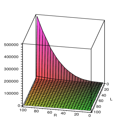
Figure 1: Case $k_{1}\simeq 0$. The masses $m_{1}$ (left) and $m_{2}$ (right) where the first derivative of the potential $V(R)$ is zero. We note that both masses are positive.

The second derivative of the potential is given by

$$\frac{d^{2}V}{dR^{2}}(R,m,L)=-\frac{1}{4R^{8}L^{4}}\left(2R^{8}L^{2}+45R^{16}-84R^{13}mL^{2}+24R^{10}m^{2}L^{4}+4R^{5}mL^{4}+21L^{4}\right).$$ (37)

 

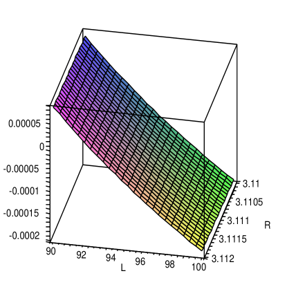
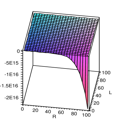
Figure 2: Case $k_{1}\simeq 0$. The second derivative of the potential $\frac{d^{2}V}{dR^{2}}(R,m,L)$ calculated at $m=m_{1}$ (left) and $m=m_{2}$ (right). We note that $\frac{d^{2}V}{dR^{2}}(R,m=m_{1},L)$ can be positive or negative (the frontier between the two regions is given by equation (39)) and that $\frac{d^{2}V}{dR^{2}}(R,m=m_{2},L)$ is always negative.

Figure 3: The possible type of potentials.

Substituting equation (35) into equation (37) we have

$$\frac{d^{2}V}{dR^{2}}(R,m=m_{1},L)=-\frac{1}{16L^{4}R^{8}}\times$$

$$\left(-2R^{8}L^{2}-27R^{16}-21R^{8}\sqrt{9R^{16}-2R^{8}L^{2}+25L^{4}}+125L^{4}+5L^{2}\sqrt{9R^{16}-2R^{8}L^{2}+25L^{4}}\right).$$

Solving $\frac{d^{2}V}{dR^{2}}(R,m=m_{1},L)=0$ we get

$$L_{f}^{2}\approx 0.9731857906R^{8}.$$ (39)

Substituting equation (36) into equation (37) we have

$$\frac{d^{2}V}{dR^{2}}(R,m=m_{2},L)=-\frac{1}{16L^{4}R^{8}}\times$$

$$\left(-2R^{8}L^{2}-27R^{16}+21R^{8}\sqrt{9R^{16}-2R^{8}L^{2}+25L^{4}}+125L^{4}-5L^{2}\sqrt{9R^{16}-2R^{8}L^{2}+25L^{4}}\right).$$

Thus, we can see from Fig. 2 that the second derivative of the potential is always positive at $m=m_{1}$ and negative at $m=m_{2}$. This means that the form of the potential is given by Figs. 3a and 3b.

Substituting equation (35) into equation (33) we have

$$V(R,m=m_{1},L)=-\frac{1}{64L^{4}R^{6}}\times$$

$$\left(46R^{8}L^{2}+25L^{4}+5L^{2}\sqrt{9R^{16}-2R^{8}L^{2}+25L^{4}}-32R^{6}L^{4}+9R^{16}+3R^{8}\sqrt{9R^{16}-2R^{8}L^{2}+25L^{4}}\right),$$

and substituting equation (36) into equation (33) we get

$$V(R,m=m_{2},L)=-\frac{1}{64L^{4}R^{6}}\times$$

$$\left(46R^{8}L^{2}+25L^{4}-5L^{2}\sqrt{9R^{16}-2R^{8}L^{2}+25L^{4}}-32R^{6}L^{4}+9R^{16}-3R^{8}\sqrt{9R^{16}-2R^{8}L^{2}+25L^{4}}\right).$$

Thus, from Fig. 4 we can see that the potential is always negative at both $m=m_{1}$ and $m=m_{2}$. This means that the form of the potential is given by the lowest curves of Figs. 3a and 3b, respectively. Hence, the collapse can either form gravastars or black holes.

 

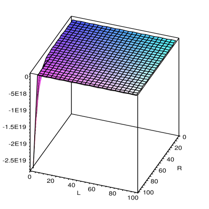
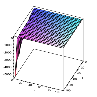
Figure 4: Case $k_{1}\simeq 0$. The potential $V(R,m,L)$ calculated at $m=m_{1}$ (left) and at $m=m_{2}$ (right). We note that both potentials are negative.

Figure 5: Case $k_{1}\simeq 0$. The potential $V(R,m,L)$ calculated at $m=m_{1}$, $R_{c}=2$ and $L_{c}=5$. This represents the formation of a ”bounded excursion” gravastar.

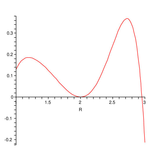
Figure 6: Case $k_{1}\simeq 0$. The potential $V(R,m,L)$ calculated at $m=m_{1}$, $R_{c}=2$ and $L_{c}=5.324211511$. This represents the formation of a stable gravastar.

Figure 7: Case $k_{1}\simeq 0$. The potential $V(R,m,L)$ calculated at $m=m_{2}$, $R_{c}=2$ and $L_{c}=10$. This represents the formation of a black hole.

IV Gravastars/Black Holes when The Thin Shell Mass Increases

Now, let us assume that $k_{1}=-2$. Then, we find that

$$V(R,m,L)=-\frac{1}{8L^{4}R^{4}}\left(-4R^{4}L^{4}+2L^{2}R^{6}+4m^{2}L^{4}-4mL^{2}R^{3}+4R^{3}L^{4}m+R^{6}+R^{6}L^{4}\right).$$ (43)

Note again that $\lim_{R\rightarrow 0}V(R,m,L)=\lim_{R\rightarrow\infty}V(R,m,L)=-\infty$.

The first derivative of the potential, equation (43), is given by

$$\frac{dV}{dR}=-\frac{1}{4L^{4}R^{5}}\left(2L^{2}R^{6}+2mL^{2}R^{3}-2R^{3}L^{4}m+R^{6}+R^{6}L^{4}-8m^{2}L^{4}\right).$$ (44)

Thus, the solutions for $\frac{dV}{dR}=0$ are

$$m_{1}=\frac{R^{3}}{8L^{2}}\left(1-L^{2}+\sqrt{9+14L^{2}+9L^{4}}\right)$$ (45)

and

$$m_{2}=\frac{R^{3}}{8L^{2}}\left(1-L^{2}-\sqrt{9+14L^{2}+9L^{4}}\right).$$ (46)

Note from Fig. 8 that $m_{2}$ is always negative, while $m_{1}$ is always positive. Since the mass must be always positive, thus the unique reasonable solution for $\frac{dV}{dR}=0$ is given by $m_{1}$.

 

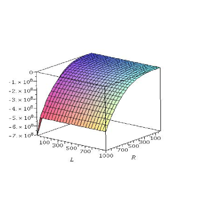
Figure 8: Case $k_{1}=-2$. The masses $m_{1}$ (left) and $m_{2}$ (right) where the first derivative of the potential $V(R)$ is zero. We can note that $m_{1}$ is always positive and $m_{2}$ is always negative. Thus, we have only $m_{1}$ as solution of $\frac{dV}{dR}=0$

The second derivative of the potential is given by

$$\frac{d^{2}V}{dR^{2}}(R,m,L)=-\frac{1}{4R^{6}L^{4}}\left(2L^{2}R^{6}-4mL^{2}R^{3}+4R^{3}L^{4}m+R^{6}+R^{6}L^{4}+40m^{2}L^{4}\right).$$ (47)

Figure 9: Case $k_{1}=-2$. The second derivative of the potential $\frac{d^{2}V}{dR^{2}}(R,m,L)$ calculated at $m=m_{1}$. We note that $\frac{d^{2}V}{dR^{2}}(R,m=m_{1},L)$ is always negative.

Thus, from Fig. 9 we can see that the second derivative of the potential is always negative at $m=m_{1}$. This means that the form of the potential is given by Fig. 3b.

Substituting equation (45) into equation (47) we have

$$\frac{d^{2}V}{dR^{2}}(R,m=m_{1},L)=-\frac{3}{16L^{4}}\times$$

$$\left(14L^{2}+9+\sqrt{9+14L^{2}+9L^{4}}+9L^{4}-L^{2}\sqrt{9+14L^{2}+9L^{4}}\right).$$

Substituting equation (45) into equation (43) we have

$$V(R,m=m_{1},L)=-\frac{1}{64L^{4}}\times$$

$$\left(-32L^{4}+30R^{2}L^{2}+9R^{2}-3R^{2}\sqrt{9+14L^{2}+9L^{4}}+9L^{4}R^{2}+3R^{2}L^{2}\sqrt{9+14L^{2}+9L^{4}}\right).$$

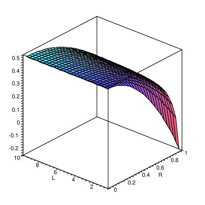
Figure 10: Case $k_{1}=-2$. The potential $V(R,m,L)$ calculated at $m=m_{1}$. We note that $V(R,m=m_{1},L)$ can be positive or negative.

We notice that $V(R,m=m_{1},L)$ can be positive or negative, depending on the radius $R$ and the cosmological constant $L$ (see figure 10). This means that there exist possibilities of formation of both gravastars and black holes.

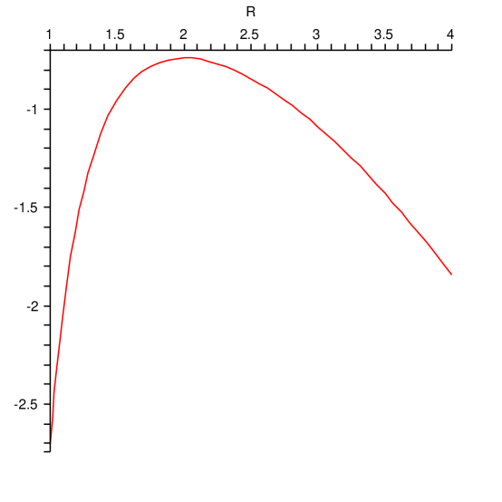
Figure 11: Case $k_{1}=-2$. The potential $V(R,m,L)$ calculated at $m=m_{1}$, $R_{c}=2$ and $L_{c}=10$. This represents the formation of a black hole.

IV.1 Total Gravitational Mass

In order to study the gravitational effect generated by the two components of the gravastar, i.e., the interior de Sitter and the thin shell in the exterior region, we need to calculate the total gravitational mass of a spherical symmetric system. Some alternative definitions are given by Marder ,Israel and Levi . Here we consider the Tolman’s formula for the mass, which is given by

$$M_{G}=\int_{0}^{R_{0}}\int_{-\pi}^{\pi}\int_{0}^{2\pi}\sqrt{-g}\;T^{\alpha}_{\alpha}drd\theta d\phi,$$ (50)

where $\sqrt{-g}$ is the determinant of the metric. For the special case of a thin shell we have

$$M_{G}=\int_{0}^{R_{0}}\int_{-\pi}^{\pi}\int_{0}^{2\pi}\sqrt{-g}\;T^{\alpha}_{\alpha}\delta({\bf r}-R_{0})d{\bf r}d\theta d\phi.$$ (51)

Thus, the Tolman’s gravitational mass of the thin shell is given by

$$M_{G}^{shell}=3M,$$ (52)

and for the interior de Sitter (dS) spacetime we have

$$M_{G}^{dS}=-\frac{2}{3}\Lambda_{i}R_{0}^{3}.$$ (53)

Thus, the de Sitter interior presents a negative gravitational mass, since $\Lambda_{i}>0$, in agreement with its repulsive effect.

Now we can write the total Tolman’s gravitational mass of the gravastar as

$$M_{G}^{total}=M_{G}^{shell}+M_{G}^{dS}=3M-\frac{2}{3}\Lambda_{i}R_{0}^{3}.$$ (54)

This mass should also represent the Vaidya exterior mass ($m=M_{G}^{total}$) of the gravastar. This last equation can explain how the mass of the shell can increase with the time. Since $m$ must decrease with the time because of the emission of radiation, the unique way that $M$ may increase with the time is that the radius $R_{0}$ is increasing with the time.

V Gravastars/Black Holes when The Thin Shell Mass Decreases

Now, let us assume that $k_{1}=+1$. Then, we find

$$V(R,m,L)=-\frac{1}{8L^{4}R^{4}}\left(-4L^{4}R^{4}+2R^{6}L^{2}+R^{12}-4R^{9}mL^{2}+4R^{6}m^{2}L^{4}+4L^{4}mR^{3}+L^{4}\right).$$ (55)

Note again that $\lim_{R\rightarrow 0}V(R,m,L)=\lim_{R\rightarrow\infty}V(R,m,L)=-\infty$.

The first derivative of the potential, equation (55), is given by

$$\frac{dV}{dR}=-\frac{1}{2L^{4}R^{5}}\left(R^{6}L^{2}+2R^{12}-5R^{9}mL^{2}+2R^{6}m^{2}L^{4}-L^{4}mR^{3}-L^{4}\right).$$ (56)

Thus the solutions for $\frac{dV}{dR}=0$ are

$$m_{1}=\frac{1}{4R^{3}L^{2}}\left(5R^{6}+L^{2}+\sqrt{9R^{12}+2R^{6}L^{2}+9L^{4}}\right),$$ (57)

and

$$m_{2}=\frac{1}{4R^{3}L^{2}}\left(5R^{6}+L^{2}-\sqrt{9R^{12}+2R^{6}L^{2}+9L^{4}}\right).$$ (58)

We note from equation (57) that $m_{1}$ is always positive and from Fig. 12 that $m_{2}$ may be positive or negative, depending on the radius $R$ and the cosmological constant $L$.

Figure 12: Case $k_{1}=+1$. The mass $m_{2}$, where the first derivative of the potential $V(R)$ is zero. We note from equation (57) that $m_{1}$ is always positive. However, $m_{2}$ can be positive or negative.

The second derivative of the potential is given by

$$\frac{d^{2}V}{dR^{2}}(R,m,L)=-\frac{1}{2R^{6}L^{4}}\left(R^{6}L^{2}+14R^{12}-20R^{9}mL^{2}+2R^{6}m^{2}L^{4}+2L^{4}mR^{3}+5L^{4}\right).$$ (59)

 

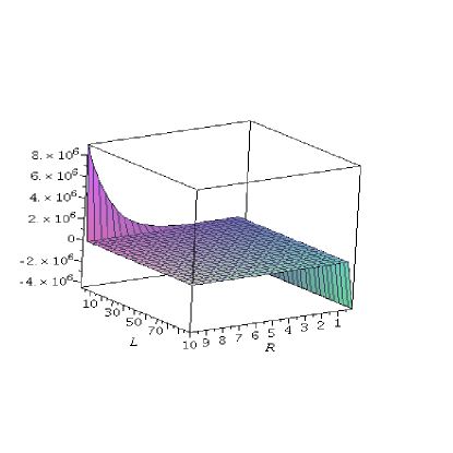
Figure 13: Case $k_{1}=+1$. The second derivative of the potential $\frac{d^{2}V}{dR^{2}}(R,m,L)$ calculated at $m=m_{1}$ (left) and at $m=m_{2}$ (right). We note that $\frac{d^{2}V}{dR^{2}}(R,m=m_{1},L)$ can be positive or negative (the frontier between the two regions is given by equation (62)) and that $\frac{d^{2}V}{dR^{2}}(R,m=m_{2},L)$ is always negative.

Thus, we can see from Fig. 13 that the second derivative of the potential can be positive or negative at $m=m_{1}$, depending on the radius $R$ and the cosmological constant $L$. This means that the form of the potential is given by Figs. 3a and 3b, respectively. Besides, the second derivative of the potential is always negative at $m=m_{2}$. This means that the form of the potential is given by Fig. 3b.

Substituting equation (57) into equation (59) we have

$$\frac{d^{2}V}{dR^{2}}(R,m=m_{1},L)=-\frac{3}{8L^{4}R^{6}}\times$$

$$\left(9R^{12}+5R^{6}\sqrt{9R^{12}+2R^{6}L^{2}+9L^{4}}-9L^{4}-L^{2}\sqrt{9R^{12}+2R^{6}L^{2}+9L^{4}}\right),$$

and substituting equation (58) into equation (59) we get

$$\frac{d^{2}V}{dR^{2}}(R,m=m_{2},L)=-\frac{3}{8L^{4}R^{6}}\times$$

$$\left(-9R^{12}+5R^{6}\sqrt{9R^{12}+2R^{6}L^{2}+9L^{4}}+9L^{4}-L^{2}\sqrt{9R^{12}+2R^{6}L^{2}+9L^{4}}\right).$$

Solving $\frac{d^{2}V}{dR^{2}}(R,m=m_{1},L)=0$, we get

$$L_{f}^{2}\approx 1.816997838R^{6}.$$ (62)

Substituting equation (57) into equation (55) we have

$$V(R,m=m_{1},L)=-\frac{1}{16L^{4}R^{4}}\times$$

$$\left(-8L^{4}R^{4}+18R^{6}L^{2}+9R^{12}+3R^{6}\sqrt{9R^{12}+2R^{6}L^{2}+9L^{4}}+9L^{4}+3L^{2}\sqrt{9R^{12}+2R^{6}L^{2}+9L^{4}}\right),$$

and substituting equation (58) into equation (55) we get

$$V(R,m=m_{2},L)=-\frac{1}{16L^{4}R^{4}}\times$$

$$\left(-8L^{4}R^{4}+18R^{6}L^{2}+9R^{12}-3R^{6}\sqrt{9R^{12}+2R^{6}L^{2}+9L^{4}}+9L^{4}-3L^{2}\sqrt{9R^{12}+2R^{6}L^{2}+9L^{4}}\right).$$

 

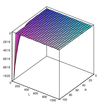
Figure 14: Case $k_{1}=+1$. The potential $V(R,m,L)$ calculated at $m=m_{1}$ (left) and at $m=m_{2}$ (right). We note that $V(R,m=m_{1},L)$ is always negative and that $V(R,m=m_{2},L)$ can be positive or negative.

Figure 15: Case $k_{1}=+1$. The potential $V(R,m,L)$ calculated at $m=m_{1}$, $R_{c}=2$ and $L_{c}=5.75$. This represents the formation of a ”bounded excursion” gravastar.

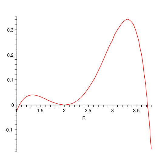
Figure 16: Case $k_{1}=+1$. The potential $V(R,m,L)$ calculated at $m=m_{1}$, $R_{c}=2$ and $L_{c}=5.907256196$. This represents the formation of a stable gravastar.

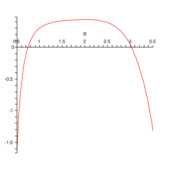
Figure 17: Case $k_{1}=+1$. The potential $V(R,m,L)$ calculated at $m=m_{2}$, $R_{c}=2$ and $L_{c}=5.75$. This represents the formation of a black hole.

We notice that $V(R,m=m_{1},L)$ is always negative (see figure 14). Since $V(R,m=m_{2},L)$ can be positive or negative, depending on the radius $R$ and the cosmological constant $L$, we may have again formation of gravastars or black holes.

VI Conclusions

In this paper, we have studied the problem of the stability of gravastars by constructing dynamical three-layer models of VW VW04 , which consists of an internal de Sitter spacetime, a dynamical infinitely thin shell of perfect fluid with the equation of state $p=\sigma$, and an external Vaidya’s spacetime.

We have shown explicitly that the final output can be a black hole, an unstable gravastar, a stable gravastar or a ”bounded excursion” gravastar, depending on the time evolution of the shell mass, the parameter $L$ and the initial position $R_{0}$ of the dynamical shell.

References

(1) P.O. Mazur and E. Mottola, ”Gravitational Condensate Stars: An Alternative to
Black Holes,” arXiv:gr-qc/0109035; Proc. Nat. Acad. Sci. 101, 9545
(2004) [arXiv:gr-qc/0407075].
(2) I. Dymnikova and E. Galaktionov, Phys. Lett. B 645,358 (2007).
(3) M. Visser and D.L. Wiltshire, Class. Quantum Grav. 21, 1135 (2004)[arXiv:gr-qc/0310107].
(5) A. DeBenedictis, et al, Class. Quantum Grav. 23, 2303 (2006) [arXiv:gr-qc/0511097].
(6) C.B.M.H. Chirenti and L. Rezzolla, arXiv:0706.1513.
(7) P. Rocha, A.Y. Miguelote, R. Chan, M.F.A. da Silva, N.O. Santos,and A. Wang,
”Bounded excursion stable gravastars and black holes,” J.
Cosmol. Astropart. Phys. 6, 25 (2008) [arXiv:gr-qc/08034200].
(8) P. Rocha, R. Chan, M.F.A. da Silva and A. Wang,
”Stable and ”Bounded Excursion” Gravastars, and Black Holes in Einstein’s Theory of Gravity,”
J. Cosmol. Astropart. Phys. 11, 10 (2008) [arXiv:gr-qc/08094879].
(9) R. Chan, M.F.A. da Silva, P. Rocha and A. Wang,
”Stable Gravastars with Anisotropic Dark Energy,”
J. Cosmol. Astropart. Phys. 3, 10 (2009) [arXiv:gr-qc/08124924].
(10) R. Chan, M.F.A. da Silva and P. Rocha,
”How the cosmological constant affects gravastar formation,”
J. Cosmol. Astropart. Phys. 12, 17 (2009) [arXiv:gr-qc/09102054].
(11) R. Chan and M.F.A. da Silva,
”How the charge can affect the formation of gravastars,”
J. Cosmol. Astropart. Phys. 7, 29 (2010) [arXiv:gr-qc/10053703].
(12) R. Chan, M.F.A. da Silva and Rocha, P.,
”Gravastars and black holes of anisotropic dark energy,”
Gen. Rel. Grav. 43, 2223 (2011) [arXiv:gr-qc/10094403].
(13) R. Chan, M.F.A. da Silva, J.F. Villas da Rocha, Gen. Relat. Grav. 41, 1835 (2009) [arXiv:gr-qc/08033064].
(14) O. Bertolami and J. Páramos, Phys. Rev. D 72, 123512
(2005) [arXiv:astro-ph/0509547]
(15) F. Lobo (2007) [arXiv:gr-qc/0611083].
(16) C. Cattoen, T. Faber and M. Visser, Class. Quantum Grav. 22
4189 (2005).
(17) V. Dzhunushaliev, V. Folomeev, R. Myrzakulov and D. Singleton, Journal of High Energy Physics 7, 94 (2008), [arXiv:gr-qc/arXiv:0805.3211].
(18) F. Lobo, Class. Quant. Grav. 23, 1525 (2006).
(19) U. Debnath and S. Chakraborty (2006) [arXiv:gr-qc/0601049].
(20) R.G. Cai and A. Wang Phys. Rev. D73, 063005 (2006)[arXiv:astro-ph/0505136].
(21) K.A. Bronnikov and J.C. Fabris, Phys. Rev. Lett. 96, 251101, (2006).
(22) K.A. Bronnikov, H. Dehnen and V.N. Melnikov, Gen. Rel. Grav. 39, 973 (2007).
(23) K. Lake, Phys. Rev. D 19, 2847 (1979).
(24) L. Marder, Proc. R. Soc. London, Ser. A, 224, 524 (1958).
(25) W. Israel, Phys. Rev. D 15, 935 (1977).
(26) A. Wang, M.F.A. da Silva and N.O. Santos, Class. Quantum Grav. 14, 2417, (1997).