Shape fluctuations in the ground and excited $0^{+}$ states
of ³⁰Mg and ³²Mg

Abstract

Large-amplitude collective dynamics of shape phase transition in the low-lying states of ^30-36Mg is investigated by solving the five-dimensional (5D) quadrupole collective Schrödinger equation. The collective masses and potentials of the 5D collective Hamiltonian are microscopically derived with use of the constrained Hartree-Fock-Bogoliubov plus local quasiparticle RPA method. Good agreement with the recent experimental data is obtained for the excited $0^{+}$ states as well as the ground bands. For ³⁰Mg, the shape coexistence picture that the deformed excited $0^{+}$ state coexists with the spherical ground state approximately holds. On the other hand, large-amplitude quadrupole-shape fluctuations dominate in both the ground and the excited $0^{+}$ states in ³²Mg, so that the interpretation of ‘coexisting spherical excited $0^{+}$ state’ based on the naive inversion picture of the spherical and deformed configurations does not hold.

Nuclei exhibit a variety of shapes in their ground and excited states. A remarkable feature of the quantum phase transition of a finite system is that the order parameters (shape deformation parameters) always fluctuate and vary with the particle number. Especially, the large-amplitude shape fluctuations play a crucial role in transitional (critical) regions. Spectroscopic studies of low-lying excited states in transitional nuclei are of great interest to observe such unique features of the finite quantum systems.

Low-lying states of neutron-rich nuclei around $N=20$ attract a great interest, as the spherical configurations associated with the magic number disappear in the ground states. In neutron-rich Mg isotopes, the increase of the excitation energy ratio $E(4_{1}^{+})/E(2_{1}^{+})$ Deacon et al. (2010); Takeuchi et al. (2009); Yoneda et al. (2001) and the enhancement of $B(E2;2^{+}_{1}\to 0^{+}_{1})$ from ³⁰Mg to ³⁴Mg Niedermaier et al. (2005); Motobayashi et al. (1995); Iwasaki et al. (2001) indicate a kind of quantum phase transition from spherical to deformed shapes taking place around ³²Mg. These experiments stimulate microscopic investigations on quadrupole collective dynamics unique to this region of the nuclear chart with various theoretical approaches; the shell model Warburton et al. (1990); Utsuno et al. (1999); Caurier et al. (2001); Otsuka (2003), the Hartree-Fock-Bogoliubov (HFB) method Terasaki et al. (1997); Reinhard et al. (1999), the parity-projected HF Ohta et al. (2005), the quasiparticle RPA (QRPA) Yamagami and Van Giai (2004); Yoshida and Yamagami (2008), the angular-momentum projected generator coordinate method (GCM) with Rodríguez-Guzmán et al. (2002) and without Yao et al. (2011a, b) restriction to the axial symmetry, and the antisymmetrized molecular dynamics Kimura and Horiuchi (2002).

Quite recently, excited $0^{+}$ states were found in ³⁰Mg Mach et al. (2005); Schwerdtfeger et al. (2009) and ³²Mg Wimmer et al. (2010) at 1.789 MeV and 1.058 MeV, respectively. For ³⁰Mg, the excited $0_{2}^{+}$ state is interpreted as a prolately deformed state which coexists with the spherical ground state. For ³²Mg, from the observed population of the excited $0_{2}^{+}$ state in the $(t,p)$ reaction on ³⁰Mg, it is suggested Wimmer et al. (2010) that the $0_{2}^{+}$ state is a spherical state coexisting with the deformed ground state and that their relative energies are inverted at $N=20$. However, available shell-model and GCM calculations considerably overestimate its excitation energy ($1.4-3.1$ MeV) Caurier et al. (2001); Otsuka (2003); Rodríguez-Guzmán et al. (2002); Schwerdtfeger et al. (2009). It is therefore a challenge for modern microscopic theories of nuclear structure to clarify the nature of the excited $0_{2}^{+}$ states. For understanding shape dynamics in low-lying collective excited states of Mg isotopes near $N=20$, it is certainly desirable to develop a theory capable of describing various situations in a unified manner, including, at least, 1) an ideal shape coexistence limit where the wave function of an individual quantum state is well localized in the deformation space and 2) a transitional situation where the large-amplitude shape fluctuations dominate.

In this article, we microscopically derive the five-dimensional (5D) quadrupole collective Hamiltonian using the constrained Hartree-Fock-Bogoliubov (CHFB) plus local QRPA (LQRPA) method Hinohara et al. (2010). The 5D collective Hamiltonian takes into account all the five quadrupole degrees of freedom: the axial and triaxial quadrupole deformations $(\beta,\gamma)$ and the three Euler angles. This approach is suitable for our purpose of describing a variety of quadrupole collective phenomena in a unified way. Another advantage is that the time-odd mean-field contributions are taken into account in evaluating the vibrational and rotational inertial functions. In spite of their importance for correctly describing collective excited states, the time-odd contributions are ignored in the widely used Inglis-Belyaev cranking formula for inertial functions. The CHFB + LQRPA method has been successfully applied to various large-amplitude collective dynamics including the oblate-prolate shape coexistence phenomena in Se and Kr isotopes Hinohara et al. (2010); Sato and Hinohara (2011), the $\gamma$-soft dynamics in $sd$-shell nuclei Hinohara and Kanada-En’yo (2011), and the shape phase transition in neutron-rich Cr isotopes Yoshida and Hinohara (2011). A preliminary version of this work was reported in Ref. Hinohara et al. (2011).

The 5D quadrupole collective Hamiltonian is written as

$${\cal H}_{\rm coll} =T_{\rm vib}+T_{\rm rot}+V(\beta,\gamma),$$ (1)

$$T_{\rm vib} =\frac{1}{2}D_{\beta\beta}(\beta,\gamma)\dot{\beta}^{2}+D_{\beta\gamma}(\beta,\gamma)\dot{\beta}\dot{\gamma}+\frac{1}{2}D_{\gamma\gamma}(\beta,\gamma)\dot{\gamma}^{2},$$ (2)

$$T_{\rm rot} =\frac{1}{2}\sum_{k=1}^{3}{\cal J}_{k}(\beta,\gamma)\omega_{k}^{2},$$ (3)

where $T_{\rm vib}$ and $T_{\rm rot}$ are the vibrational and rotational kinetic energies, respectively, and $V$ is the collective potential. The vibrational collective masses, $D_{\beta\beta},D_{\beta\gamma}$, and $D_{\gamma\gamma}$, are the inertial functions for the $(\beta,\gamma)$ coordinates. The rotational moments of inertia ${\cal J}_{k}$ associated with the three components of the rotational angular velocities $\omega_{k}$ are defined with respect to the principal axes. In the CHFB + LQRPA method, the collective potential is calculated with the CHFB equation with four constraints on the two quadrupole operators and the proton and neutron numbers. The inertial functions in the collective Hamiltonian are determined from the LQRPA normal modes locally defined for each CHFB state in the $(\beta,\gamma)$ plane. The equations to find the local normal modes are similar to the well-known QRPA equations, but the equations are solved on top of the non-equilibrium CHFB states. Two LQRPA solutions representing quadrupole shape motion are selected for the calculation of the vibrational inertial functions. After quantizing the collective Hamiltonian (1), we solve the 5D collective Schrödinger equation and obtain collective wave functions

$$\Psi_{\alpha IM}(\beta,\gamma,\Omega)=\sum_{K={\rm even}}\Phi_{\alpha IK}(\beta,\gamma)\langle\Omega|IMK\rangle,$$ (4)

where $\Phi_{\alpha IK}(\beta,\gamma)$ are the vibrational wave functions and $\langle\Omega|IMK\rangle$ are the rotational wave functions defined in terms of ${\cal D}$ functions ${\cal D}^{I}_{MK}(\Omega)$. We then evaluate $E2$ matrix elements. More details of this approach are given in Ref. Hinohara et al. (2010).

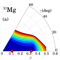
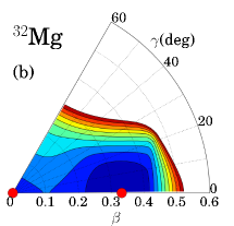
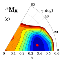
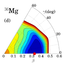
Figure 1: (Color online) Collective potentials for ^30-36Mg. The HFB equilibrium points are indicated by red circles.

We solve the CHFB + LQRPA equations employing, as a microscopic Hamiltonian, the pairing-plus-quadrupole (P+Q) model including the quadrupole-pairing interaction. As an active model space, the two-major harmonic oscillator shells ($sd$ and $pf$ shells) are taken into account for both neutrons and protons. To determine the parameters in the P+Q Hamiltonian, we first perform Skyrme-HFB calculations with the SkM* functional and the surface pairing functional using the HFBTHO code Stoitsov et al. (2005). The pairing strength ($V_{0}=-374$ MeV fm^-3, with a cutoff quasiparticle energy of 60 MeV) is fixed so as to reproduce the experimental neutron gap of ³⁰Ne (1.26 MeV). We then determine the parameters for each nucleus in the following way. The single particle energies are determined by means of the constrained Skyrme-HFB calculation at the spherical shape. The resulting single particle energies (in the canonical basis) are then scaled with the effective mass of the SkM* functional $m^{*}/m=0.79$, since the P+Q model is designed to be used for single-particle states whose effective mass is equal to the bare nucleon mass. In ³²Mg, the $N=20$ shell gap between $d_{3/2}$ and $f_{7/2}$ is 3.7 MeV for the SkM* functional, and it becomes 2.9 MeV after the effective mass scaling. This value is appreciably smaller than the standard modified oscillator value 4.5 MeV Bengtsson and Ragnarsson (1985). This spacing almost stays constant for ^30-36Mg. The strengths of the monopole-pairing interaction are determined to reproduce the pairing gaps obtained in the Skyrme-HFB calculations at the spherical shape. The strength of the quadrupole particle-hole interaction is determined to reproduce the magnitude of the axial quadrupole deformation $\beta$ of the Skyrme-HFB minimum. The strengths of the quadrupole-pairing interaction are determined so as to fulfill the self-consistency condition Sakamoto and Kishimoto (1990). We use the quadrupole polarization charge $\delta e_{\rm pol}=0.5$ for both neutrons and protons when evaluating $E2$ matrix elements. We solve the CHFB + LQRPA equations at 3600 $\beta$-$\gamma$ mesh points in the region $0<\beta<\beta_{\rm max}$ and $0^{\circ}<\gamma<60^{\circ}$, with $\beta_{\rm max}=0.5$ for ³⁰Mg and 0.6 for ^32,34,36Mg.

Our theoretical framework is quite general and it can be used in conjunction with various Skyrme forces/modern density functionals going beyond the P+Q model. Then the effects of weakly bound neutrons and coupling to the continuum on the properties of the low-lying collective excitations, discussed in Refs. Yamagami and Van Giai (2004); Yoshida and Yamagami (2008), can be taken into account, for example, by solving the CHFB + LQRPA equations in the 3D coordinate mesh representation. However, it requires a large-scale calculation with modern parallel processors and it remains as a challenging future subject. A step toward this goal has recently been carried out for axially symmetric cases Yoshida and Hinohara (2011).

Figure 1 shows the collective potentials $V(\beta,\gamma)$ for ^30-36Mg. It is clearly seen that prolate deformation grows with increase of the neutron number. The collective potential for ³⁰Mg is very soft with respect to $\beta$. It has a minimum at $\beta=0.11$ and a local minimum at $\beta=0.33$. The barrier height between the two minima is only 0.24 MeV (measured from the lower minimum). In ³²Mg, in addition to the prolate minimum at $\beta=0.33$, a spherical local minimum (associated with the $N=20$ spherical shell gap) appears. The barrier height between the two minima is 1.0 MeV (measured from the lower minimum). The spherical local minimum disappears in ³⁴Mg and ³⁶Mg, and the prolate minima become soft in the direction of triaxial deformation $\gamma$. In ³⁴Mg, the potential minimum is located at $\gamma=10^{\circ}$.

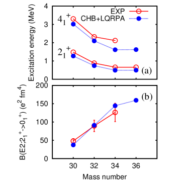
Figure 2: (Color online) Comparison of calculated excitation energies of the $2_{1}^{+}$ and $4_{1}^{+}$ states (upper panel) and $B(E2;2_{1}^{+}\to 0_{1})$ values (lower panel) in ^30-36Mg with experimental data Deacon et al. (2010); Takeuchi et al. (2009); Yoneda et al. (2001); Niedermaier et al. (2005); Motobayashi et al. (1995); Iwasaki et al. (2001).

In Fig. 2, calculated excitation energies and $E2$ transition strengths are compared with the experimental data. The lowering of the excitation energies of the $2_{1}^{+}$ and $4_{1}^{+}$ states and the remarkable increase of $B(E2;2_{1}^{+}\to 0_{1}^{+})$ from ³⁰Mg to ³⁴Mg are well described in this calculation. The calculated ratio of the excitation energies, $E(4_{1}^{+})/E(2_{1}^{+})$, increases as 2.37, 2.82, 3.26, and 3.26, while the ratio of the transition strengths, $B(E2;4_{1}^{+}\to 2_{1}^{+})/B(E2;2_{1}^{+}\to 0_{1}^{+})$, decreases as 2.03, 1.76, 1.43, and 1.47, in going from ³⁰Mg to ³⁶Mg. Thus, the properties of the $2_{1}^{+}$ and $4_{1}^{+}$states gradually change from vibrational to rotational with increasing neutron number.

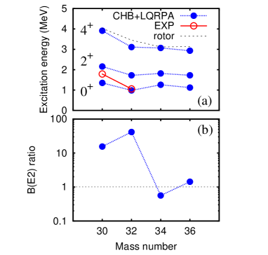
Figure 3: (Color online) Excitation energies of the excited $0_{2}^{+}$, $2_{2,3}^{+}$ and $4_{2,3}^{+}$ states (upper panel) and the ratio $B(E2;0_{2}^{+}\to 2_{1}^{+})/B(E2;0_{1}^{+}\to 2^{+}_{2,3})$ of the inter-band $E2$ transition strengths between the $K=0_{2}$ and $K=0_{1}$ bands (lower panel). Experimental data are taken from Refs. Schwerdtfeger et al. (2009); Wimmer et al. (2010). See texts for details.

Let us next discuss the properties of the $0^{+}_{2}$ states and the $2^{+}$ and $4^{+}$ states connected to the $0_{2}^{+}$ states with strong $E2$ transitions. The result of calculation is presented in Fig. 3 together with the recent experimental data. The calculated excitation energies of the $0_{2}^{+}$ states are 1.353 and 0.986 MeV for ³⁰Mg and ³²Mg, respectively, in fair agreement with the experimental data Schwerdtfeger et al. (2009); Wimmer et al. (2010). In particular, the very low excitation energy of the $0_{2}^{+}$ state in ³²Mg is well reproduced. In our calculation, more than 90% (80%) of the collective wave functions for the yrast (excited) band members are composed of the $K=0$ component. Therefore we denote the ground band by ‘the $K=0_{1}$ band,’ and the excited band by ‘the $K=0_{2}$ band.’ The $2^{+}$ and $4^{+}$ states belonging to the $K=0_{2}$ band appear as the second $2^{+}$ and $4^{+}$ states in ^30,32Mg, while they appear as the third $2^{+}$ and $4^{+}$ states in ^34,36Mg. Accordingly, we use $2^{+}_{2,3}$ and $4^{+}_{2,3}$, to collectively indicate the second or the third $2^{+}$ and $4^{+}$ states. The calculated ratios of the excitation energies relative to the excited $0_{2}^{+}$ state, $[E(4_{2,3}^{+})-E(0_{2}^{+})]/[E(2_{2,3}^{+})-E(0_{2}^{+})]$, are 3.18, 2.87, 3.25, and 3.00, for ³⁰Mg, ³²Mg, ³⁴Mg, and ³⁶Mg, respectively. In the upper panel of Fig. 3 we also plot the rotor-model prediction for the excitation energies of the $4^{+}$ states estimated from the $0^{+}-2^{+}$ spacings in the $K=0_{2}$ bands. The deviation from the rotor-model prediction is largest in ³²Mg indicating importance of shape-fluctuation effects. Although the calculated excitation spectrum of the $K=0_{2}$ band in ³⁰Mg looks rotational, we find a significant deviation from the rotor-model prediction in the $E2$ transition properties. The calculated ratios of the $E2$ transition strengths, $B(E2;4_{2,3}^{+}\to 2_{2,3}^{+})/B(E2;2_{2,3}^{+}\to 0^{+}_{2})$, are 1.05, 1.54, 1.47, and 1.51, for ^30-36Mg, respectively. The deviation from the rotor-model value (1.43) is largest in ³⁰Mg. The significant deviation from the simple rotor-model pattern of the $K=0_{2}$ bands in ³⁰Mg and ³²Mg, noticed above, can be seen more drastically in the inter-band $E2$ transition properties. In the lower panel of Fig. 3, we plot the ratio $B(E2;0_{2}^{+}\to 2_{1}^{+})/B(E2;0_{1}^{+}\to 2^{+}_{2,3})$ of the inter-band transition strengths between the $K=0_{1}$ and $K=0_{2}$ bands. If the $K=0_{1}$ and $K=0_{2}$ bands are composed of only the $K=0$ component and the intrinsic structures in the $(\beta,\gamma)$ plane are the same within the band members, this ratio should be one. These ratios for ³⁴Mg and ³⁶Mg are close to one, indicating that the change of the intrinsic structure between the $0^{+}$ and $2^{+}$ states is small. In contrast, the ratios for ³⁰Mg and ³²Mg are larger than 10, indicating a remarkable change in the shape-fluctuation properties between the $0^{+}$ and $2^{+}$ states belonging to the $K=0_{1}$ and $K=0_{2}$ bands.

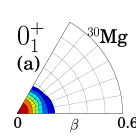
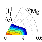
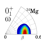
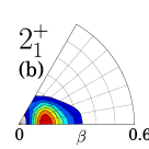
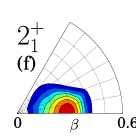
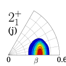
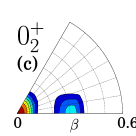
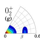
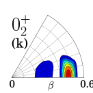
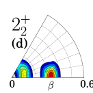
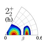
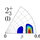
Figure 4: (Color online) Vibrational wave functions squared $\sum_{K}|\Phi_{\alpha IK}(\beta,\gamma)|^{2}$ of the $0_{1}^{+},2_{1}^{+},0_{2}^{+}$ and $2^{+}_{2,3}$ states in ^30-34Mg. Contour lines are drawn at every eighth part of the maximum value.

Figure 4 shows the vibrational wave functions squared $\sum_{K}|\Phi_{\alpha IK}(\beta,\gamma)|^{2}$. Let us first examine the character change of the ground state from ³⁰Mg to ³⁴Mg. In ³⁰Mg, the vibrational wave function of the ground $0_{1}^{+}$ state is distributed around the spherical shape. In ³²Mg, it is remarkably extended to the prolately deformed region. In ³⁴Mg, it is distributed around the prolate shape. From the behavior of the vibrational wave functions, one can conclude that shape fluctuation in the ground $0_{1}^{+}$ state is largest in ³²Mg. To understand the microscopic mechanism of this change from ³⁰Mg to ³⁴Mg, it is necessary to take into account not only the properties of the collective potential in the $\beta$ direction but also its curvature in the $\gamma$ direction and the collective kinetic energy (collective masses). This point will be discussed in our forthcoming full-length paper. As suggested from the behavior of the inter-band $B(E2)$ ratio, the vibrational wave functions of the $2_{1}^{+}$ state are noticeably different from those of the $0_{1}^{+}$ state in ³⁰Mg and ³²Mg, while they are similar in the case of ³⁴Mg. Next, let us examine the vibrational wave functions of the $0_{2}^{+}$ and $2_{2,3}^{+}$ states in ^30-34Mg. It is immediately seen that they exhibit one node in the $\beta$ direction. This is their common feature. In ³⁰Mg and ³²Mg, one bump is seen in the spherical to weakly-deformed region, while the other bump is located in the prolately deformed region around $\beta=0.3-0.4$. In ³⁴Mg, the node is located near the peak of the vibrational wave function of the $0_{1}^{+}$ state, suggesting that they have $\beta$-vibrational properties.

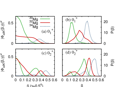
Figure 5: (Color online) (a) Vibrational wave functions squared, $|\Phi_{\alpha,I=0,K=0}(\beta,\gamma=0.5^{\circ})|^{2}$, of the $0_{1}^{+}$ states in ^30-34Mg. Their values along the $\gamma=0.5^{\circ}$ line are plotted as functions of $\beta$. (b) Probability densities integrated over $\gamma$, $P(\beta)\equiv\int d\gamma|\Phi_{\alpha,I=0,K=0}(\beta,\gamma)|^{2}|G(\beta,\gamma)|^{1/2}$, of the $0_{1}^{+}$ states in ^30-34Mg, plotted as functions of $\beta$. (c) Same as (a) but for the $0_{2}^{+}$ states. (d) Same as (b) but for the $0_{2}^{+}$ states.

To further reveal the nature of the ground and excited $0^{+}$ states, it is important to examine not only their vibrational wave functions but also their probability density distributions. Since the 5D collective space is a curved space, the normalization condition for the vibrational wave functions is given by

$$\int\sum_{K}|\Phi_{\alpha IK}(\beta,\gamma)|^{2}|G(\beta,\gamma)|^{1/2}d\beta d\gamma=1$$ (5)

with the volume element

$$|G(\beta,\gamma)|^{1/2}d\beta d\gamma=2\beta^{4}\sqrt{W(\beta,\gamma)R(\beta,\gamma)}\sin 3\gamma d\beta d\gamma,$$ (6)

$$W(\beta,\gamma)= \{D_{\beta\beta}(\beta,\gamma)D_{\gamma\gamma}(\beta,\gamma)-[D_{\beta\gamma}(\beta,\gamma)]^{2}\}\beta^{-2},$$ (7)

$$R(\beta,\gamma)= D_{1}(\beta,\gamma)D_{2}(\beta,\gamma)D_{3}(\beta,\gamma),$$ (8)

where $D_{k=1,2,3}$ are the rotational masses defined through ${\cal J}_{k}=4\beta^{2}D_{k}\sin^{2}(\gamma-2\pi k/3)$. Thus, the probability density of taking a shape with specific values of ($\beta,\gamma$) is given by $\sum_{K}|\Phi_{\alpha IK}(\beta,\gamma)|^{2}|G(\beta,\gamma)|^{1/2}$. Due to the $\beta^{4}$ factor in the volume element, the spherical peak of the vibrational wave function disappears in the probability density distribution. Accordingly, it will give us a picture quite different from that of the wave function. Needless to say, it is important to examine both aspects to understand the nature of individual quantum states.

In Fig. 5, we display the probability density integrated over $\gamma$, $P(\beta)\equiv\int d\gamma|\Phi_{\alpha,I=0,K=0}(\beta,\gamma)|^{2}|G(\beta,\gamma)|^{1/2}$, of finding a shape with a specific value of $\beta$, together with the vibrational wave functions squared $|\Phi_{\alpha,I=0,K=0}(\beta,\gamma)|^{2}$ for the ground and excited $0^{+}$ states ($\alpha=1$ and 2). Let us first look at the upper panels for the ground states. We note that, as expected, the spherical peak of the vibrational wave function for ³⁰Mg in Fig. 5(a) corresponds to the peak at $\beta\simeq 0.15$ of the probability density in Fig. 5(b). In Fig. 5(b), the peak position moves toward a larger value of $\beta$ in going from ³⁰Mg to ³⁴Mg. The distribution for ³²Mg is much broader than those for ³⁰Mg and ³⁴Mg.

Next, let us look at the lower panels in Fig. 5 for the excited states. In Fig. 5(c). the vibrational wave functions for ³⁰Mg and ³²Mg exhibit the maximum peak at the spherical shape. However, these peaks become small and are shifted to the region with $\beta\simeq 0.1$ and $\beta\simeq 0.2$ in ³⁰Mg and ³²Mg, respectively, in Fig. 5(d). On the other hand, the second peaks at $\beta\simeq 0.3$ and $\beta\approx 0.4$ in ³⁰Mg and ³²Mg, respectively, seen in Fig. 5(c) become the prominent peaks in Fig. 5(d). In ³⁰Mg, the bump at $\beta\simeq 0.1$ is much smaller than the major bump around $\beta\simeq 0.3$. In this sense, we can regard the $0_{2}^{+}$ state of ³⁰Mg as a prolately deformed state. In the case of ³²Mg, the probability density exhibits a very broad distribution extending from the spherical to deformed regions up to $\beta=0.5$ with a prominent peak at $\beta\simeq 0.4$ and a node at $\beta\simeq 0.3$. The position of the node coincides with the peak of the probability density distribution of the the $0_{1}^{+}$ state, as expected from the orthogonality condition. The range of the shape fluctuation of the $0_{2}^{+}$ state in $\beta$ direction is almost the same as that of the $0_{1}^{+}$ state. Thus, the result of our calculation yields a physical picture for the $0_{2}^{+}$ state in ³²Mg that is quite different from the ‘spherical excited $0^{+}$ state’ interpretation based on the inversion picture of the spherical and deformed configurations. In ³⁴Mg, the peak is shifted to the region with a larger value of $\beta$ and the tail toward the spherical shape almost disappears.

In summary, we have investigated the large-amplitude collective dynamics in the low-lying states of ^30-36Mg by solving the 5D quadrupole collective Schrödinger equation. The collective masses and potentials of the 5D collective Hamiltonian are microscopically derived with use of the CHFB + LQRPA method. Good agreement with the recent experimental data is obtained for the excited $0^{+}$ states as well as the ground bands. For ³⁰Mg, the shape coexistence picture that the deformed excited $0^{+}$ state coexists with the spherical ground state approximately holds. On the other hand, large-amplitude quadrupole-shape fluctuations dominate in both the ground and the excited $0^{+}$ states in ³²Mg, so that the interpretation of ‘deformed ground and spherical excited $0^{+}$ states’ based on the simple inversion picture of the spherical and deformed configurations does not hold. To test these theoretical predictions, experimental search for the distorted rotational bands built on the excited $0_{2}^{+}$ states in ³⁰Mg and ³²Mg is strongly desired.

One of the authors (N. H.) is supported by the Special Postdoctoral Research Program of RIKEN. The numerical calculations were performed on the RIKEN Integrated Cluster of Clusters (RICC). This work is supported by KAKENHI (Nos. 21340073, 20105003, 23540234, and 23740223).

References

- Deacon et al. (2010) A. N. Deacon et al., Phys. Rev. C 82, 034305 (2010).
- Takeuchi et al. (2009) S. Takeuchi et al., Phys. Rev. C 79, 054319 (2009).
- Yoneda et al. (2001) K. Yoneda et al., Phys. Lett. B 499, 233 (2001).
- Niedermaier et al. (2005) O. Niedermaier et al., Phys. Rev. Lett. 94, 172501 (2005).
- Motobayashi et al. (1995) T. Motobayashi et al., Phys. Lett. B 346, 9 (1995).
- Iwasaki et al. (2001) H. Iwasaki et al., Phys. Lett. B 522, 227 (2001).
- Warburton et al. (1990) E. K. Warburton et al., Phys. Rev. C 41, 1147 (1990).
- Utsuno et al. (1999) Y. Utsuno et al., Phys. Rev. C 60, 054315 (1999).
- Caurier et al. (2001) E. Caurier et al., Nucl. Phys. A 693, 374 (2001).
- Otsuka (2003) T. Otsuka, Eur. Phys. J. A 20, 69 (2003).
- Terasaki et al. (1997) J. Terasaki et al., Nucl. Phys. A 621, 706 (1997).
- Reinhard et al. (1999) P.-G. Reinhard et al., Phys. Rev. C 60, 014316 (1999).
- Ohta et al. (2005) H. Ohta et al., Eur. Phys. J. A 25, s1.549 (2005).
- Yamagami and Van Giai (2004) M. Yamagami et al., Phys. Rev. C 69, 034301 (2004).
- Yoshida and Yamagami (2008) K. Yoshida et al., Phys. Rev. C 77, 044312 (2008).
- Rodríguez-Guzmán et al. (2002) R. Rodríguez-Guzmán et al., Nucl. Phys. A 709, 201 (2002).
- Yao et al. (2011a) J. M. Yao et al., Phys. Rev. C 83, 014308 (2011a).
- Yao et al. (2011b) J. M. Yao et al., Int. J. Mod. Phys. E 20, 482 (2011b).
- Kimura and Horiuchi (2002) M. Kimura et al., Prog. Theor. Phys. 107, 33 (2002).
- Mach et al. (2005) H. Mach et al., Eur. Phys. J. A 25, 105 (2005).
- Schwerdtfeger et al. (2009) W. Schwerdtfeger et al., Phys. Rev. Lett. 103, 012501 (2009).
- Wimmer et al. (2010) K. Wimmer et al., Phys. Rev. Lett. 105, 252501 (2010).
- Hinohara et al. (2010) N. Hinohara et al., Phys. Rev. C 82, 064313 (2010).
- Sato and Hinohara (2011) K. Sato et al., Nucl. Phys. A 849, 53 (2011).
- Hinohara and Kanada-En’yo (2011) N. Hinohara et al., Phys. Rev. C 83, 014321 (2011).
- Yoshida and Hinohara (2011) K. Yoshida et al., Phys. Rev. C 83, 061302 (2011).
- Hinohara et al. (2011) N. Hinohara et al., AIP Conf. Proc. 1355, 200 (2011), eprint arXiv:1101.2256.
- Stoitsov et al. (2005) M. Stoitsov et al., Comp. Phys. Comm. 167, 43 (2005).
- Bengtsson and Ragnarsson (1985) T. Bengtsson et al., Nucl. Phys. A 436, 14 (1985).
- Sakamoto and Kishimoto (1990) H. Sakamoto et al., Phys. Lett. B 245, 321 (1990).