LSPM J1112+7626: detection of a 41-day M-dwarf eclipsing binary from the MEarth transit survey

Abstract

We report the detection of eclipses in LSPM J1112+7626, which we find to be a moderately bright ($I_{C}=12.14\pm 0.05$) very low-mass binary system with an orbital period of $41.03236\pm 0.00002\ \rm days$, and component masses $M_{1}=0.395\pm 0.002\ {\rm M}_{\odot}$ and $M_{2}=0.275\pm 0.001\ {\rm M}_{\odot}$ in an eccentric ($e=0.239\pm 0.002$) orbit. A $65\ \rm day$ out of eclipse modulation of approximately $2\%$ peak-to-peak amplitude is seen in $I$-band, which is probably due to rotational modulation of photospheric spots on one of the binary components. This paper presents the discovery and characterization of the object, including radial velocities sufficient to determine both component masses to better than $1\%$ precision, and a photometric solution. We find that the sum of the component radii, which is much better-determined than the individual radii, is inflated by $3.8^{+0.9}_{-0.5}\%$ compared to the theoretical model predictions, depending on the age and metallicity assumed. These results demonstrate that the difficulties in reproducing observed M-dwarf eclipsing binary radii with theoretical models are not confined to systems with very short orbital periods. This object promises to be a fruitful testing ground for the hypothesized link between inflated radii in M-dwarfs and activity.

1. Introduction

Detached, double-lined eclipsing binaries (EBs) provide a largely model-independent means to precisely and accurately measure fundamental stellar properties, particularly masses and radii. In the best-observed systems the precision of these can be at the $<1$ per cent level, and thus place stringent constraints on stellar evolution models (e.g. Andersen 1991; Torres et al. 2010).

Despite the ubiquity of M-dwarfs in the solar neighborhood, their fundamental properties are poorly understood. This is particularly the case below $0.35\ {\rm M}_{\odot}$, the boundary at which field stars are thought to become fully convective (e.g. Chabrier & Baraffe 1997). Furthermore, observations of many of the best-characterized M-dwarf EBs indicate significant discrepancies with the stellar models.

The components of CM Dra, the best characterized double-lined system in the fully-convective mass range (Eggen & Sandage, 1967; Lacy, 1977; Metcalfe et al., 1996; Morales et al., 2009), have radii approximately $5-7\%$ larger than predicted by theoretical stellar evolution models. The observation of inflated radii for M-dwarf binaries at the $5-10\%$ level, and effective temperatures $3-5\%$ lower than the models predict, is nearly ubiquitous among the best-characterized objects (e.g. Torres et al. 2010, and references therein; Morales et al. 2010; Kraus et al. 2011), although it is interesting to note that Carter et al. (2011) find a smaller inflation for KOI-126B and C, members of a fascinating system containing a short-period M-dwarf binary orbiting a K-star, where the system undergoes mutual eclipses allowing a precise determination of the radii of both M-dwarfs.

Two main hypotheses have been advanced to explain the inflated radii in low-mass eclipsing binaries: metallicity (Berger et al., 2006), and the effect of magnetic activity (the “activity hypothesis”, e.g. López-Morales & Ribas 2005; Ribas 2006; Chabrier et al. 2007).

As discussed by López-Morales (2007), one of the main difficulties with metallicity as an explanation is that current models of M-dwarfs yield radii differing only by a very small amount (an increase of approximately $3\%$) between $[{\rm M/H}]=-0.5$ to $0$, the range spanned by the available Baraffe et al. (1998) models. Unless the EB sample contains many objects of very high metallicity, this effect does not seem large enough.

Observationally, the difficulty of determining metallicities for M-dwarfs (e.g. Bonfils et al. 2005; Woolf & Wallerstein 2006; Bean et al. 2006) renders the metallicity hypothesis difficult to test in practice, and this is further exacerbated by the double lines and rapid rotation in most M-dwarf eclipsing binary spectra. Nonetheless, it is interesting to note that CM Dra is thought to be metal poor (Viti et al., 1997, 2002), which would increase the size of the radius discrepancy for this object, rather than decreasing it, and more generally, this is expected to also be true of other eclipsing binaries in the sample, assuming they follow the metallicity distribution of field stars (e.g. Carney et al. 1989).

Given these lines of reasoning, it seems unlikely that metallicity is the only explanation for the inflated radii (although it probably plays a role, particularly in creating scatter in the effective temperatures). This has led to the “activity hypothesis” becoming the preferred explanation in the literature for the inflation. It is motivated by noting that nearly all EB systems have short orbital periods. For example, below $0.35\ {\rm M}_{\odot}$, the longest period system is 1RXS J154727.5+450803 at $3.55\ {\rm days}$ (Hartman et al., 2011). At such short periods, the components are expected to have been tidally synchronized and the orbits circularized by field ages. The effect of the companion and tidal locking is likely to significantly increase the activity levels. The available observational evidence supports this, with the eclipsing binaries below $0.35\ {\rm M}_{\odot}$ all showing signs of high activity and tidal effects including synchronous, rapid rotation, large amplitude out of eclipse modulations, H$\alpha$ emission, X-ray emission, and in most cases, circular orbits.

Magnetic activity could have an effect either by inhibiting convection (Mullan & MacDonald, 2001; Chabrier et al., 2007), or due to reduced heat flux resulting from cool photospheric spots. Of these, Chabrier et al. (2007) find the structure of objects below $0.35\ {\rm M}_{\odot}$ is almost independent of variations in the mixing length parameter, which they use to implement inhibition of convection, so the latter possibility (inhibition of radiation due to the effect of spots) seems more likely the explanation in the mass domain of particular interest here. It is important to note that spots also influence the solution of eclipsing binary light curves. The possibility of such systematic errors in the observations is discussed by Morales et al. (2010), and we shall return to it later in the analysis.

An obvious way to test the activity hypothesis is to measure radii for components of eclipsing binaries with long orbital periods, where tides are unimportant, and the stars should rotate close to the rates expected for single stars in the absence of a binary companion. Unfortunately, such an endeavor is difficult due to the reduced geometric alignment probability and limited availability of long-duration photometric monitoring of M-dwarfs at rapid cadences, where the majority of wide-field variability surveys are carried out in visible bandpasses, often yielding poor signal to noise ratios for M-dwarfs, which are faint at these wavelengths.

The longest-period M-dwarf EB with a published orbit is T-Lyr1-17236 (Devor et al., 2008), which has an $8.4\ \rm day$ orbital period and components of $0.68$ and $0.52\ {\rm M}_{\odot}$. The radii are indeed consistent with the theoretical models, but the observational uncertainties are still quite large in the discovery paper. This object is currently being observed by the NASA Kepler mission, so a more precise solution should be forthcoming.

In light of the difficulty of identifying longer-period EBs, several authors have attempted to test the activity hypothesis using the existing EB sample to search for correlations between e.g. orbital period or activity measures and radius inflation (López-Morales, 2007; Kraus et al., 2011). While there does appear to be evidence for such a correlation above $0.35\ {\rm M}_{\odot}$, below this mass the present sample is limited by small number statistics and the narrow range of orbital periods spanned. The Kepler mission appears to have identified a large number of very long-period EB systems (Prša et al. 2011; see also Coughlin et al. 2011 where more detailed solutions using the Kepler photometry are presented for low-mass objects from this sample), but we are not aware of published dynamical masses and model-independent radii for these at the present time, and many of the M-dwarfs (especially below $0.35\ {\rm M}_{\odot}$) are secondaries in systems with mass ratios much less than unity, where detecting the secondary spectrum to measure radial velocities may be challenging.

An alternative method to determine M-dwarf radii is by making interferometric measurements of angular diameters for (usually isolated) stars. Combined with trigonometric parallaxes and minor assumptions about the stellar limb darkening, the physical radius of the star can be inferred in a model-independent fashion. The difficulty with this method comes in estimating the stellar mass. Dynamical measurements are usually not available, so one has to resort to inferring mass from other measurable stellar properties, necessarily with larger uncertainties. Typically, absolute magnitude in near-infrared passbands is used, which is found to correlate well with stellar mass and has a relatively small scatter. The empirical polynomials of Delfosse et al. (2000) are the most widely used, although there is some argument in the literature as to how accurately these predict the mass, especially over a range of metallicity and spectral type (the uncertainties are probably $\geq 10\%$). These concerns combined with small sample sizes mean interferometry results have thus far remained somewhat ambiguous (e.g. Demory et al. 2009; Boyajian et al. 2011, and references therein).

In this contribution, we present the discovery of eclipses in LSPM J1112+7626, a nearby double-lined M-dwarf system with an extremely long orbital period (compared to existing well-characterized M-dwarf EBs) of approximately $41\ \rm days$. At this large orbital separation the system is not expected to have experienced significant tidal effects (e.g. Zahn 1977), and is predicted to be neither synchronized nor circularized, as verified by the non-circular orbit and apparent non-synchronized spin and orbit for one of the components as we shall describe. In the absence of strong tidal effects, it is expected that the angular momentum evolution of each component has not been perturbed significantly by the binary companion, and therefore the stars should possess magnetic properties more representative of single M-dwarfs. In this contribution, we proceed to derive a high-quality spectroscopic orbit and a photometric solution for the system.

2. Observations and data reduction

2.1. Initial detection

LSPM J1112+7626 was targeted as part of routine operation of the MEarth transit survey (Nutzman & Charbonneau, 2008; Irwin et al., 2009a) during the 2009-2010 season, with the first observations taken on UT 2009 December 2. Exposure times for the LSPM J1112+7626 field were $27\ {\rm s}$, taking three exposures per visit (the total exposure times are tailored for each target to achieve sensitivity to a particular planet size for the assumed stellar radius), with visits at a cadence of $20\ {\rm minutes}$.

Eclipses were first detected in LSPM J1112+7626 on UT 2010 April 3 (this was a primary eclipse), and subsequently confirmed on UT 2010 April 28th by observing the majority of a secondary eclipse egress. Both eclipses were detected by an experimental automated real-time eclipse detection and followup system we began to trial during the 2009-2010 season (this will be described in detail in a future publication when it has matured). Confident that the object was an eclipsing binary, but still with an ambiguous orbital period, we immediately commenced radial velocity monitoring. The radial velocities ultimately determined which of the possible orbital periods was correct, in conjunction with a further eclipse (which was also a secondary) observed on UT 2010 June 8 with MEarth and the Clay telescope (see §2.2).

2.2. Secondary eclipses

By the time the orbital ephemeris was well-known, the observing season on LSPM J1112+7626 from Arizona was ending, and the weather had begun to deteriorate due to the arrival of the monsoon. We therefore took advantage of the high declination of our target and commenced an observing program to target the secondary eclipses using the Harvard University $0.4$m Landon T. Clay telescope, which is located on the roof of the Science Center on the Harvard campus near Harvard Square, Cambridge, Massachusetts. This instrument is normally used for undergraduate teaching. It is equipped with an e2v CCD47-10 $1024\times 1024$ pixel back-illuminated CCD packaged by Apogee Instruments (model AP47), which was operated binned $2\times 2$ for a final pixel scale of $\approx 1\farcs 59$ per pixel to reduce overheads.

The location of the telescope is extremely light polluted, and combined with the red colors of our target, we decided to use the $I$-band filter to mitigate the effects of sky background and atmospheric extinction. The filter available was built to the prescription of Bessell (1990) using Schott RG9 glass to define the bandpass, and shall hereafter be referred to as $I_{\rm Bessell}$. While this filter was intended to approximate the Cousins $I$ passband (hereafter $I_{C}$), the combination of the glass filter and CCD quantum efficiency yields a system response with significant sensitivity at very red wavelengths not present in the original Cousins passband, and thus is a poor approximation to the Cousins filter for very red stars such as M-dwarfs. We shall return to this issue in §4.4.

Data were successfully gathered using the Clay telescope for the secondary eclipses on UT 2010 June 8, October 9, November 19, and December 30th. The entire eclipse was visible for all but the June 8th event, although varying fractions of these were lost due to clouds. Exposure times were adjusted to keep the peak counts in the target below $30\,000$ to avoid saturation, and ranged from $30-60\ {\rm s}$. The typical cadence was $50\ {\rm s}$ and the FWHM of the stellar images was $2-3$ binned pixels. No guiding was available, so the target was re-centered manually approximately every $20$ exposures to attempt to keep the drift below $5$ pixels.

Data were reduced and light curves produced using standard procedures for CCD data, following the method outlined in Irwin et al. (2007). 2-D bias frames were subtracted as there was some bias structure evident, and we used the overscan region to correct for any bias level variations. Dark frames of exposure matched to the target frames were subtracted to correct for the (significant) dark current and hot pixels at the $-20$C operating temperature of the CCD, and the data were flat-fielded using twilight flat-fields in the usual way. No defringing or absolute calibration of the photometry were attempted. Fringing was clearly visible in the images, but at a low amplitude ($3\%$ peak-to-peak) and should not have a significant effect on the photometry due to the stabilized telescope pointing.

We present the full light curve data-set used in this paper in Table 1, and times of minimum light for the eclipses where a clear minimum was seen in Table 2.

Table 1 Light curve data.

ID	Orbit	HJD_UTC	$I$	$\sigma(I)$	$\Delta$ mag	FWHM	Airmass	MeridFlag	$x$	$y$	CM
		(days)	(mag)	(mag)	(mag)	(pix)			(pix)	(pix)	(mag)
C	$1$	$2455355.573517$	$-0.0224$	$0.0073$	$0.000$	$2.10$	$1.2814$	$0$	$100.427$	$378.595$	$0.0000$
C	$1$	$2455355.574050$	$-0.0168$	$0.0077$	$-0.002$	$2.19$	$1.2820$	$0$	$100.715$	$378.567$	$0.0000$
C	$1$	$2455355.574547$	$-0.0161$	$0.0079$	$-0.000$	$2.18$	$1.2827$	$0$	$100.936$	$378.442$	$0.0000$
C	$1$	$2455355.575091$	$-0.0176$	$0.0079$	$-0.033$	$2.26$	$1.2833$	$0$	$100.904$	$378.255$	$0.0000$
C	$1$	$2455355.575624$	$-0.0165$	$0.0081$	$-0.010$	$2.20$	$1.2840$	$0$	$100.900$	$378.023$	$0.0000$

Note. — Table 1 is published in its entirety in the electronic edition of the Astrophysical Journal. A portion is shown here for guidance regarding its form and content.

Table 2 Times of minimum light.

HJD_UTC	Uncertainty	Cycle	Eclipse	Instrument
(days)	(s)
$2455577.272644$	$7$	$7$	Primary	Hankasalmi
$2455355.627938$	$41$	$1$	Secondary	Clay
$2455478.725045$	$42$	$4$	Secondary	Clay
$2455519.757412$	$31$	$5$	Secondary	Clay
$2455560.789627$	$11$	$6$	Secondary	Clay
$2455519.757351$	$16$	$5$	Secondary	MEarth
$2455683.887000$	$20$	$9$	Secondary	MEarth

Note. — Estimated using the method of Kwee & van Woerden (1956), over an interval of $\pm 10^{-3}$ in normalized orbital phase. These times of minimum are not used in our analysis (we fit for the ephemeris directly from the data) and are reported only for completeness.

2.3. Primary eclipse

Using the timing of the single visit within the primary eclipse of UT 2010 April 3 from MEarth (see §2.1) combined with modeling of the secondary eclipses (§2.2) and radial velocities (§3) it was possible to predict the primary eclipse times with reasonable accuracy. During 2010-2011 full eclipses were observable at reasonable airmass ($<2.0$) from eastern Europe, Scandinavia, and western Asia, with the high declination of the target favoring northerly latitudes during winter to maximize dark hours at reasonable airmass.

The primary eclipse was observed using the $40\ {\rm cm}$ telescope at Hankasalmi Observatory, Finland on UT 2011 January 15, starting approximately 10 minutes before first contact, and continuing until well after last contact. Data were taken using a similar $I_{\rm Bessell}$ filter to the secondary eclipse observations (see §2.2) with a front-illuminated Kodak KAF-1001E CCD packaged by Santa Barbara Instrument Group (SBIG; model STL-1001E). This system response should be very similar to the one used for the secondary eclipses, but nonetheless, any bandpass mismatch is a potential concern for the accuracy of the photometric solution when combining data taken with different instruments, and will be discussed in more detail in §4.4.

Exposure times of $60\ {\rm s}$ were used, yielding a cadence of approximately $2$ minutes, and the target was re-centered every $10$ exposures to keep the drift below $\approx 50$ pixels. Data were reduced using 2-D bias frames, and master dark and flat-field frames. Light curves were then derived using the same methods and software as for the other data-sets.

2.4. Out of eclipse and additional secondary eclipses

Following the discovery of atmospheric water vapor induced systematic effects in the MEarth photometry (see Irwin et al. 2011), a customized $I$-band filter was procured for the start of the 2010-2011 season, with a bandpass designed to eliminate the strong telluric water vapor absorption at wavelengths $>900\ {\rm nm}$, by using an $895\ {\rm nm}$ ($50\%$ transmittance point) interference cutoff on the same RG715 glass substrate as the original filter (where the long-pass glass filter defines the blue end of the bandpass). This was predicted to reduce the effect to largely insignificant levels, and the resulting system response approximates the Cousins $I$ bandpass (as tabulated by Bessell 1990; see later in this section).

Observations of LSPM J1112+7626 using this new filter commenced on UT 2010 October 29, and continued until UT 2011 May 18. Exposures of $2\times 97\ {\rm s}$ were used at $20\ {\rm minute}$ cadence for times out of eclipse. $5283$ useful data points were obtained at airmasses $<2$, after discarding $400$ bad frames (pointing errors, severe light loss due to clouds, and large scatter in the zeropoint solution for the differential photometry).

Partial secondary eclipses were obtained with the same MEarth telescope on UT 2010 November 19, UT 2011 February 9, and UT 2011 May 2. Due to known systematic effects caused by persistence in the MEarth CCDs, leading to offsets in magnitude depending on the cadence (see Berta et al. 2011), and to remove any residual from the out-of-eclipse variations, we allow these high-cadence observations to have different photometric zero-points than the out of eclipse data (and each other) in the final light curve analysis.

The out-of-eclipse data (excluding the high-cadence eclipse observations) were searched for periodic variations using the method outlined in Irwin et al. (2011). Correction for the “common mode” effect was still performed, as we discovered during the season that replacing the filters had in fact increased the size (and changed the sign) of the systematic effect rather than eliminating it. This problem is still under investigation, but we suspect it is due to humidity and/or temperature dependence of the filter bandpass, an effect also seen in the original Sloan Digital Sky Survey (SDSS) Photometric Telescope filters (Doi et al., 2010).

After correcting for the “common mode” effect, the MEarth data show a strong near-sinusoidal modulation with a $65\ \rm day$ period (see Figure 1; the data are shown in §4) and a peak-to-peak amplitude of approximately $0.02\ {\rm mag}$. Marginal evidence for a similar periodicity is found in the 2009-2010 data, although the phase is not consistent and the amplitude appears to be much smaller. It is unclear if the amplitude change results from the differing filter systems, but the change in phase (if real) may be indicative of evolution of the photospheric spot patterns giving rise to the modulations.

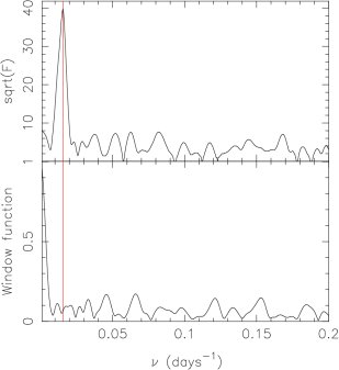
Figure 1.— “F-test periodogram” for the MEarth 2010-2011 season out of eclipse observations, plotting the square root of the F-test statistic comparing the null hypothesis of no variation to the alternate hypothesis of a sinusoidal modulation, as a function of frequency (top) and the corresponding window function (bottom). The vertical line indicates the best-fitting period of $64.8\ \rm days$.

An improvement resulting from the new MEarth filter is a greatly reduced color term when standardizing the photometry onto the Cousins system. The scatter in this relation also appears to be significantly lower, which may also result in part from improvements made to our flat-fielding strategy during the 2010-2011 season. The MEarth observing software automatically obtains measurements of equatorial photometric standard star fields from the catalog of Landolt (1992) every night, and these are used to derive photometric zero-points and calibrated photometry. The typical scatter in these zero-point solutions on a photometric night is $0.02\ {\rm mag}$. We find a typical atmospheric extinction of $0.05\ {\rm mag/airmass}$ from MEarth data, which has been assumed henceforth.

A significant issue with the equatorial standard fields is they contain very few red stars suitable for defining the red end of the photometric response, and so color equations derived only from these equatorial fields may be significantly in error when attempting to standardize M-dwarf photometry. Thankfully, MEarth serendipitously targeted a number of M-dwarfs with photometry available on the Cousins system from Bessel (1990). We selected all such objects in the 2010-2011 MEarth database with data available on photometric nights for calibration. Two objects with clearly unreliable MEarth data were discarded, leaving $8$ objects. The following color equation was derived from these stars, which span $I_{C}-K_{\rm 2MASS}$ colors of $2.2-4.2$:

$$I_{C}=I_{\rm MEarth} - (0.085\pm 0.019)$$

$$+ (0.0204\pm 0.0064)\ (I_{\rm MEarth}-K_{\rm 2MASS})$$

In the case of LSPM J1112+7626, we estimate $I_{C}=12.14\pm 0.05$ using this relation, where we have inflated the uncertainty to account for variability and any errors introduced by the varying MEarth bandpass as discussed above. The observed $I_{C}-J$, $I_{C}-H$ and $I_{C}-K$ colors are later used to infer effective temperatures and luminosities for the members of the binary, and thus the distance to the system.

2.5. Literature data: proper motion and photometry

In Table 3, we summarize the photometric and astrometric system properties gathered from literature data and our photometry. This star lies within the area covered by the Sloan Extension for Galactic Understanding and Evolution (SEGUE) stripe 1260 photometry, so we retrieved the PSF magnitudes from Data Release 7 (Abazajian et al., 2009). This object is flagged as saturated in $i$-band (the image also shows a very unusual PSF and may be corrupted), and the $u$-band photometry of M-dwarfs in SDSS is corrupted by a well-documented red leak problem, so we omit these filters.

Table 3 Summary of the photometric and astrometric properties of the LSPM J1112+7626 system.

Parameter	Value
$\alpha_{2000}$	$11^{h}12^{m}42^{s}.35$
$\delta_{2000}$	$+76^{\circ}26\arcmin 56\farcs 3$
$\mu_{\alpha}\cos\delta$	$0\farcs 131\ {\rm yr^{-1}}$
$\mu_{\delta}$	$-0\farcs 108\ {\rm yr^{-1}}$
$g$	$15.618\pm 0.010$
$r$	$14.195\pm 0.012$
$z$	$12.027\pm 0.012$
$I_{\rm C}$	$12.14\pm 0.05$
$J_{\rm 2MASS}$	$10.591\pm 0.023$
$H_{\rm 2MASS}$	$9.989\pm 0.021$
$K_{\rm 2MASS}$	$9.728\pm 0.017$

The moderately high proper motion of our target allows the contribution of any background objects to the system light to be constrained using previous epochs of imaging. In Figure 2, we show imaging data with the position and size of the MEarth photometric aperture (which is representative of the aperture sizes used for all the photometry) overlaid. The DSS1 image indicates the aperture is unlikely to contain any significant flux from background objects, and the SDSS image (which has the highest angular resolution) does not appear elongated.

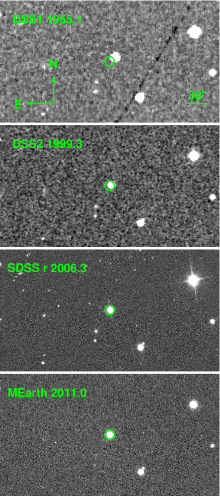
Figure 2.— Images of LSPM J1112+7626 centered on the position as measured from the MEarth data. The circle shows the approximate position and size of the $8\arcsec$ (radius) photometric aperture used to derive the MEarth light curves. Data are from the first and second epoch Palomar sky surveys as provided by the Digitized Sky Survey (DSS; top and center panels), SDSS, and the MEarth master image (bottom panel). The approximate epochs are shown on the images, and all four panels have the same center, scale and alignment on-sky.

2.6. Intermediate-resolution optical spectroscopy: spectral typing and metallicity constraints

A single epoch intermediate-resolution ($R\simeq 1200$) spectrum of our target was obtained using the FLWO $1.5\ {\rm m}$ Tillinghast reflector and FAST spectrograph (Fabricant et al., 1998) on UT 2011 March 16. The default setting of a $300\ {\rm g/mm}$ grating and $3\arcsec$ slit was used to obtain two exposures of $300\ {\rm s}$. The spectra were reduced using standard procedures for long slit spectra in IRAF (Tody, 1993), using a HeNeAr arc exposure taken inbetween the two target exposures to ensure accurate wavelength calibration. The 2-D spectra were divided by a flat field before extraction to remove the majority of the fringing seen at the reddest wavelengths. Relative flux calibration was performed using the spectrophotometric standard BD+26 2606. We show the resulting spectra in Figure 3.

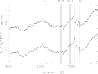
Figure 3.— Intermediate-resolution FAST spectra of LSPM J1112+7626 showing the TiO and CaH molecular bands typically used for M-dwarf spectral classification. Two exposures were obtained and are shown offset in the vertical direction for clarity. Overlaid in gray are the locations of the H$\alpha$ line, and the CaH2, CaH3 and TiO5 band indices defined by Reid et al. (1995).

Using the TiO5 band index defined by Reid et al. (1995), we find a composite spectral type of M3.7 (note that the uncertainty in this value is at least $0.5$ subclass), and using The Hammer (Covey et al., 2007), we find M3-M4 (visual inspection indicates the observed spectrum is closer to M4). The spectral type and the measured colors are in good agreement using the empirical colors of Galactic disk M-dwarfs from Leggett (1992) for the Johnson/Cousins/CIT system and West et al. (2005) for the SDSS/2MASS.

It is also clear from Figure 3 that no H$\alpha$ line is seen in the spectrum. Such behavior is typical of inactive field dwarfs at these spectral types when observed at low resolution, where the equivalent width of the H$\alpha$ absorption line becomes close to zero at M4-M5 (e.g. Gizis et al. 2002; see their Figure 5, noting that the TiO5 index was $0.42$ for LSPM J1112+7626). The presence of H$\alpha$ emission in M-dwarf spectra is usually indicative of high activity levels.

The relative strengths of the TiO and CaH bands in optical spectra have been used to identify and classify M-subdwarfs (Gizis, 1997), and more generally proposed as a method for estimating metallicities of M-dwarfs (e.g. Woolf & Wallerstein 2006). While detailed calibrations (e.g. using band indices) do not yet appear to be available, we performed a visual comparison between Figure 3 and the spectra shown in Gizis (1997). The strong TiO bands seen in our target indicate it is not extremely metal poor. We therefore estimate it has metallicity $[{\rm Fe/H}]>-1$, and is probably closer to solar (or greater).

2.7. High-resolution optical spectroscopy: radial velocities

High-resolution spectroscopic observations were obtained using the TRES fiber-fed échelle spectrograph on the FLWO $1.5\ {\rm m}$ Tillinghast reflector. We used the medium fiber ($2\farcs 3$ projected diameter), yielding a resolving power of $R\simeq 44\,000$.

Observations commenced on UT 2010 May 1, and continued until UT 2011 April 13, with $43$ epochs acquired. Total exposure times ranged from 45 to 80 minutes, broken into sequences of 3 or 4 individual exposures. The spectra were extracted using a custom built pipeline designed to provide precise radial velocities for échelle spectrographs. The procedures are described in more detail in Buchhave et al. (2010), and will be summarized briefly below.

In order to effectively remove cosmic rays, the sets of raw images were median combined. We used a flat field to trace the échelle orders and to correct the pixel to pixel variations in CCD response and fringing in the red-most orders, then extracted one-dimensional spectra using the “optimal extraction” algorithm of Hewett et al. (1985) (see also Horne 1986). The scattered light in the two-dimensional raw image was determined and removed by masking out the signal in the échelle orders and fitting the inter-order light with a two-dimensional polynomial.

Thorium-Argon (ThAr) calibration images were obtained through the science fiber before and after each stellar observation. The two calibration images were combined to form the basis for the fiducial wavelength calibration. TRES is not a vacuum spectrograph and is only temperature controlled to $0.1{\rm{}^{\circ}C}$. Consequently, the radial velocity errors are dominated by shifts due to pressure, humidity and temperature variations. In order to successfully remove these large variations ($>1.5\ \rm km\ s^{-1}$), it is critical that the ThAr light travels along the same optical path as the stellar light and thus acts as an effective proxy to remove these variations. We have therefore chosen to sandwich the stellar exposure with two ThAr frames instead of using the simultaneous ThAr fiber, which may not exactly describe the induced shifts in the science fiber and can also lead to bleeding of ThAr light into the science spectrum from the strong argon lines, especially at redder wavelengths. The pairs of ThAr exposures were co-added to improve the signal to noise ratio, and centers of the ThAr lines found by fitting a Gaussian function to the line profiles. A two-dimensional fifth order Legendre polynomial was used to describe the wavelength solution.

3. Spectroscopic analysis

Radial velocities were obtained using the two-dimensional cross-correlation algorithm todcor (Zucker & Mazeh, 1994), which uses templates matched to each component of a spectroscopic binary to simultaneously derive the velocities of both stars, and an estimate of their light ratio in the spectral bandpass.

We used a single epoch observation of Barnard’s star (Barnard 1916; also known as Gl 699) taken on UT 2008 October 20 as the template for the todcor analysis. Barnard’s star has a spectral type of M4 (Kirkpatrick et al., 1991), which should be a reasonable match to both components. Correlations were performed using a wavelength range of 7063 to 7201Å in order 41 of the spectrum to derive the velocities, since this region contains strong molecular features (mostly from TiO), which are rich in radial velocity information. We assume a barycentric radial velocity of $-110.3\pm 0.5\ \rm km\ s^{-1}$ for Barnard’s star (where the stated uncertainty reflects our estimate of the systematic errors), derived from presently unpublished CfA Digital Speedometer measurements spanning $17\ {\rm years}$.

To derive the light ratio, we ran todcor using a range of fixed values of this quantity, seeking the maximum correlation over all epochs. In this way, consistency between the different epochs is enforced, in accordance with the expectation that the true value of this quantity should be (approximately) constant. This procedure improves the stability of the solution and minimizes systematic errors in the velocities. We find a best-fitting light ratio of $L_{2}/L_{1}=0.528\pm 0.05$, where we adopt a conservative estimate of the uncertainty.

The radial velocities derived from our analysis are reported in Table 4. We omit four velocities with peak correlation values below $C_{\rm peak}=0.5$ from the table and the remainder of the analysis as the low correlation values indicate these velocities are likely to be unreliable or to exhibit large scatter. The uncertainty in the radial velocities (estimated from our fitting procedure; see §4) is $0.26\ \rm km\ s^{-1}$ for the primary, and $0.58\ \rm km\ s^{-1}$ for the secondary, with an additional systematic uncertainty, estimated to be $0.5\ \rm km\ s^{-1}$ (see above), in the velocity zero-point system.

Table 4 Radial velocity data.

HJD_UTC	Phase	$v_{1}$	$v_{2}$	$C_{\rm peak}$
(days)		($\rm km\ s^{-1}$)	($\rm km\ s^{-1}$)
$2455317.6481$	$0.67269$	$-49.45$	$-78.49$	$0.560$
$2455320.6671$	$0.74626$	$-41.11$	$-90.08$	$0.635$
$2455321.6714$	$0.77074$	$-38.58$	$-93.77$	$0.643$
$2455341.6568$	$1.25780$	$-79.89$	$-33.62$	$0.586$
$2455342.6784$	$1.28270$	$-79.29$	$-34.71$	$0.506$
$2455343.6545$	$1.30649$	$-78.44$	$-36.09$	$0.541$
$2455344.6632$	$1.33107$	$-78.21$	$-36.76$	$0.577$
$2455345.6848$	$1.35597$	$-76.63$	$-38.66$	$0.642$
$2455346.6622$	$1.37979$	$-75.23$	$-40.34$	$0.536$
$2455347.6488$	$1.40383$	$-74.26$	$-42.12$	$0.654$
$2455348.6433$	$1.42807$	$-72.38$	$-44.19$	$0.602$
$2455366.6561$	$1.86706$	$-35.28$	$-97.31$	$0.627$
$2455367.6852$	$1.89214$	$-37.23$	$-96.02$	$0.588$
$2455368.6748$	$1.91626$	$-40.62$	$-90.98$	$0.670$
$2455369.6903$	$1.94101$	$-44.54$	$-84.52$	$0.576$
$2455373.6462$	$2.03742$	$-65.72$	$-53.84$	$0.547$
$2455374.6460$	$2.06178$	$-69.12$	$-48.82$	$0.662$
$2455375.6455$	$2.08614$	$-72.87$	$-43.53$	$0.582$
$2455581.9638$	$7.11433$	$-75.90$	$-39.72$	$0.750$
$2455582.9270$	$7.13780$	$-77.72$	$-37.42$	$0.788$
$2455583.8762$	$7.16093$	$-79.01$	$-35.40$	$0.811$
$2455584.9160$	$7.18627$	$-79.99$	$-34.08$	$0.806$
$2455586.9587$	$7.23606$	$-80.51$	$-33.75$	$0.854$
$2455587.9329$	$7.25980$	$-80.20$	$-33.98$	$0.829$
$2455605.9077$	$7.69786$	$-46.45$	$-82.16$	$0.816$
$2455606.9374$	$7.72296$	$-43.79$	$-87.07$	$0.624$
$2455607.9274$	$7.74709$	$-41.08$	$-90.00$	$0.797$
$2455608.8926$	$7.77061$	$-38.34$	$-93.22$	$0.757$
$2455611.8887$	$7.84363$	$-34.67$	$-99.11$	$0.731$
$2455614.8719$	$7.91633$	$-40.32$	$-91.05$	$0.741$
$2455615.8710$	$7.94068$	$-44.85$	$-84.66$	$0.822$
$2455616.9096$	$7.96599$	$-50.16$	$-76.85$	$0.742$
$2455617.8577$	$7.98910$	$-55.18$	$-69.76$	$0.788$
$2455650.7940$	$8.79179$	$-36.93$	$-95.63$	$0.780$
$2455651.7573$	$8.81526$	$-35.56$	$-97.88$	$0.732$
$2455652.8008$	$8.84070$	$-34.89$	$-98.32$	$0.808$
$2455656.7773$	$8.93761$	$-44.06$	$-85.15$	$0.814$
$2455659.7417$	$9.00985$	$-59.54$	$-62.78$	$0.815$
$2455664.7613$	$9.13218$	$-77.22$	$-38.03$	$0.826$

We find no evidence for “peak pulling” effects close to the systemic velocity, which might indicate the need for additional rotational broadening of the template to match the target. Barnard’s star is a very slow rotator (e.g. Benedict et al. 1998), so this and the high correlation values obtained without need for additional rotational broadening indicate both components of our target have low $v\sin i$, as expected.

4. Model

For EB systems showing moderate or high eccentricities, the commonly exploited property of being able to separate the photometric and spectroscopic solutions no longer holds as the eccentricity affects both. Typically, the orbital period $P$, epoch of primary eclipse $T_{0}$, and $e\cos\omega$ (where $e$ is eccentricity and $\omega$ is the argument of periastron) are better determined by the photometry (by eclipse timing; the latter is related to the departure of the secondary eclipses in phase from being exactly halfway between the primary eclipses, although note that the commonly-used one-to-one relation between these quantities is approximate), and the $e\sin\omega$ component is usually best constrained by the velocities (but also affects the relative durations of the two eclipses, and in general eccentricity also influences their shape). Therefore, in order to leverage the best possible constraints on the system orbit, we adopt a joint solution of all the light curves and the radial velocities simultaneously. This also greatly simplifies the error analysis.

We proceed by first discussing the basic model and assumptions in §4.1, the method of solution in §4.2, and then the effects of four potentially important sources of systematic error in the system parameters we derive: spots (§4.3), bandpass mismatch (§4.4), limb darkening (§4.5), and third light (§4.6). In §4.7, we summarize our best estimates of the system parameters and their corresponding uncertainties.

4.1. Basic model and assumptions

To model the system, we used the light curve generator from the popular jktebop code (Southworth et al., 2004a, b), which is in turn based on the eclipsing binary orbit program (ebop; Popper & Etzel 1981). This model approximates the stars using biaxial ellipsoids (Nelson & Davis, 1972), which is appropriate for well-detached systems such as the present one. We modified the model to perform the computations in double precision, to account for light travel time, which is necessary due to the large semimajor axis, and to incorporate a simple prescription for the effect of photospheric spots (discussed in §4.3). The light curve model was coupled with a standard Keplerian orbital model for the radial velocities (also including the light travel time). We correct the orbital period from the heliocentric frame to the system barycenter (Griffin et al., 1976) when computing the physical parameters, following the usual convention of reporting the orbital period $P$ as measured in the heliocentric frame (i.e. without the correction) in the tables.

We fit all of the Clay, Hankasalmi, and 2010-2011 season MEarth data, the radial velocities, and the spectroscopic light ratio simultaneously. We also include the single primary eclipse of UT 2010 April 3 to improve the constraint on the ephemeris, assuming the bandpass was approximately the same as the $I_{\rm Bessell}$ filter (this makes little difference in practice due to the sparse coverage). The remainder of the MEarth 2009-2010 season data were omitted as these are of quite poor quality and were taken in a different bandpass from the remainder, so do not usefully constrain the model after accounting for the extra free parameters which must be added in order to fit them.

Table 5 summarizes the assumptions made in our light curve model. The light curve parameter set generally follows jktebop, and has been chosen to minimize correlations between parameters where possible. We add a term $k_{l}(X-1)$ to the model magnitudes, where $X$ is airmass, and $l$ is an index for the different light curves, to account for differential atmospheric extinction between the target and comparison stars, presumably due to color-dependence. A different $k_{l}$ value was allowed for each light curve $l$. This has only been used for fitting the Clay secondary eclipse curves and 2010-2011 MEarth data (see §2.2), where it seems to be necessary to include this term to obtain an acceptable fit to the out of eclipse portions. We are unsure as to the exact origin of the baseline curvature in the Clay data, and note that the choice of a linear function of airmass is arbitrary and may not be correct. This is further evidenced by the inconsistent sign and magnitude of this term in Table 6. We suggest the best approach to rectifying this problem would be to obtain higher quality secondary eclipse observations.

Table 5 Parameters and priors used in the basic model.

Parameter	Value	Prior	Description
$J_{\rm MEarth}$	varied	uniform	Central surface brightness ratio (secondary/primary) in $I_{\rm MEarth}$
$J_{\rm Bessell}$	varied	uniform	Central surface brightness ratio (secondary/primary) in $I_{\rm Bessell}$
$(R_{1}+R_{2})/a$	varied	uniform	Total radius divided by semimajor axis
$R_{2}/R_{1}$	varied	uniform	Radius ratio
$\cos i$	varied	uniform (isotropic)	Cosine of orbital inclination
$e\cos\omega$	varied	uniform in $e$,$\omega$	Eccentricity times cosine of argument of periastron
$e\sin\omega$	varied	uniform in $e$,$\omega$	Eccentricity times sine of argument of periastron
$L_{2}/L_{1}$	$0.528\pm 0.05$	Gaussian	$I_{\rm MEarth}$-band light ratio
$u_{1}$	$-0.0765$	uniform	Primary limb darkening linear coefficient
$u^{\prime}_{1}$	$1.0369$	uniform	Primary limb darkening sqrt coefficient
$u_{2}$	$0.0561$	uniform	Secondary limb darkening linear coefficient
$u^{\prime}_{2}$	$0.9335$	uniform	Secondary limb darkening sqrt coefficient
$\beta_{1}$	$0.32$	…	Primary gravity darkening exponent
$\beta_{2}$	$0.32$	…	Secondary gravity darkening exponent
$\kappa_{1}$	computed	…	Primary reflection effect coefficient
$\kappa_{2}$	computed	…	Secondary reflection effect coefficient
$L_{3}$	$0$	uniform	Third light divided by total light
$\Phi$	$0$	…	Tidal lead/lag angle
$\delta$	$2^{\circ}$	…	Integration ring size
$F_{1}$	varied	uniform	Primary rotation parameter
$a_{1}$	varied	uniform	Primary out-of-eclipse sine coefficient
$b_{1}$	varied	uniform	Primary out-of-eclipse cosine coefficient
$F_{2}$	varied	uniform	Secondary rotation parameter
$a_{2}$	varied	uniform	Secondary out-of-eclipse sine coefficient
$b_{2}$	varied	uniform	Secondary out-of-eclipse cosine coefficient
$q$	varied	uniform	Mass ratio
$K_{1}+K_{2}$	varied	modified Jeffreys	Sum of radial velocity semiamplitudes
		$K_{a}=0.02\ \rm km\ s^{-1}$	Prior $P(K_{1}+K_{2})\propto 1/(K_{1}+K_{2}+K_{a})$
$\gamma$	varied	uniform	Systemic radial velocity
$P$	varied	uniform	Orbital period (heliocentric)
$T_{0}$	varied	uniform	Epoch of primary conjunction (HJD_UTC)
$T_{\rm sec}$	computed	…	Epoch of secondary conjunction (HJD_UTC)
$z_{l}$	varied	uniform	Baseline magnitude for light curve $l$
$s_{l}$	varied	Jeffreys	Error scaling factor for light curve $l$
$k_{l}$	varied	uniform	Airmass coefficient for light curve $l$ (where used)
$C_{l}$	varied	uniform	Common mode coefficient for light curve $l$ (where used)
$s_{r}$	varied	Jeffreys	Error (if $C_{\rm peak}=1$) for radial velocity curve $r$

Gravity darkening coefficients were fixed at values appropriate for convective atmospheres (Lucy, 1967), although gravity darkening is unimportant with the precision of the present light curves at such low rotation rates. The reflection effect was computed rather than fitting for it, although again the large semimajor axis means it is unimportant.

We used a square root limb darkening law (Diaz-Cordoves & Gimenez, 1992), of the form:

$${I_{\lambda}(\mu)\over{I_{\lambda}(1)}}=1-u(1-\mu)-u^{\prime}(1-\sqrt{\mu})$$ (1)

where $I_{\lambda}(\mu)$ is the specific intensity, and $\mu=\cos\theta$, where $\theta$ is the angle between the surface normal and the line of sight. As discussed by van Hamme (1993), the square root law is a better approximation to the specific intensity distribution given by model atmospheres of late-type stars in the NIR than the other common two-parameter laws (quadratic and logarithmic) implemented in jktebop. We also verified this by comparing the Claret (2000) four-parameter law (which we assumed to be the best representation of the original phoenix model) with the two-parameter laws for typical M-dwarf stellar parameters.

For our baseline model, we fixed the limb darkening coefficients to values for the $I_{C}$ filter derived from phoenix model atmospheres by Claret (2000), using $T_{\rm eff}=3130\ {\rm K}$ for the primary, and $T_{\rm eff}=3010\ {\rm K}$ for the secondary, $\log g=5.0$ and solar metallicity. We assume the same limb darkening law applies to all the $I$ filters (the error introduced by this assumption is examined in §4.5).

No evidence was found for any background sources in the photometric aperture (see §2.5), and the radial velocity observations do not show additional lines or velocity drifts that might indicate a comoving, physically associated companion to the EB system. We therefore assume no third light ($L_{3}=0$), but see also §4.6.

4.2. Method of solution

To derive parameters and error estimates, we adopt a variant of the popular Markov Chain Monte Carlo (MCMC) analysis frequently applied in cosmology and for analysis of exoplanet radial velocity and light curve data (e.g. Tegmark et al. 2004; Ford 2005). We use Adaptive Metropolis (Haario et al., 2001) rather than the standard Metropolis-Hastings method with the Gibbs sampler. The adaptive method allows adjustment of the proposal distributions while the chain runs, and is thus simpler and faster to operate, obviating the need for manual tuning of the proposal distributions typical of the more conventional methods. This method uses a multivariate Gaussian proposal distribution to perturb all parameters simultaneously.

Compared to the simpler Monte Carlo and bootstrapping methods (e.g. as implemented in jktebop) these methods have an important advantage for the present case where a heterogeneous set of light curves and radial velocities must be analyzed: it is possible to estimate the appropriate inflation of the observational uncertainties self-consistently and simultaneously with the other model parameters (e.g. Gregory 2005). This allows the correct relative weighting of the various observational data-sets to be decided essentially by their residuals from the best-fitting model, and the uncertainty in this weighting to be propagated to the final parameters. Of course, this assumes the correct model has been chosen for the data, so these methods must be used carefully.

In the Monte Carlo simulations, we used the standard Metropolis-Hastings acceptance criterion, accepting the new point with probability:

$$P_{\rm acc}=\left\{\begin{array}[]{r}1,P(M_{i+1}|D)\geq P(M_{i}|D)\\ {P(M_{i+1}|D)\over{P(M_{i}|D)}},P(M_{i+1}|D)<P(M_{i}|D)\end{array}\right.$$

where $P(M_{i}|D)$ and $P(M_{i+1}|D)$ are the posterior probabilities of the previous and current points, respectively, $M_{i}$ represents the $i$th model, and $D$ the data. The previous point in the chain was repeated if the new point was not accepted (this is required to correctly implement the method). The appropriate ratio of posterior probabilities (“Bayes factor”) was:

$${P(M_{i+1}|D)\over{P(M_{i}|D)}}={P(M_{i+1})\over{P(M_{i})}}\ \exp(-\Delta\chi^{2}/2)$$ (2)

where the factors in the right-hand side are the ratio of prior probabilities, and the usual (least squares) likelihood ratio, respectively.

Priors assumed for each parameter are detailed in Table 5, and are chosen to be uninformative. In most cases, this choice is a uniform improper prior (labeled “uniform” in the table). For the orbital inclination, we adopt a uniform prior on $\cos i$, which produces an isotropic distribution of orbit normals, and for the eccentricity, we use a uniform prior on $e$ and $\omega$, rather than on the jump parameters $e\cos\omega$ and $e\sin\omega$ (the latter would produce a prior in $e,\omega$ proportional to $e$; e.g. Ford 2006).

As discussed by Gregory (2005), the appropriate choice of uninformative prior for “scale parameters” such as radial velocity amplitude or orbital period is a Jeffreys prior (or a modified Jeffreys prior for parameters which can be zero). This enforces scale invariance (equal probability per decade). In the present case, some of these parameters (particularly the period) are so well-determined the choice of prior is unimportant, so for simplicity we have only used non-uniform priors on the less well-determined parameters where the prior is important.

As discussed earlier, and in Gregory (2005), it is possible to fit for the appropriate inflation of the observational uncertainties simultaneously with the model parameters. This has been done via the $s_{k}$ parameters shown in Table 5. It is conventional to apply this inflation by multiplication for light curves, and for RV by adding an extra “jitter” contribution in quadrature. We follow these conventions here. Note that additional factors appear in the likelihood ratio of Eq. (2) when doing this, which have been subsumed into the $\Delta\chi^{2}$ in the equation.

For the RV, it is difficult to estimate reliable uncertainties from cross correlation functions, so instead we derive them during the simulation. We weight each point by $C_{\rm peak}^{2}$ (the square of the peak normalized cross-correlation value; see Table 4), where we find $C_{\rm peak}$ is approximately proportional to the signal to noise ratio in typical observations at similar signal to noise and peak correlation values to those seen in this work. This procedure is essentially equivalent to photon-weighting, except the cross-correlation accounts for all sources of uncertainty rather than only photon noise. The uncertainty corresponding to a peak correlation of unity is derived during the simulation, and we allow separate values of this quantity for each star, labeled $s_{1}$ for the primary, and $s_{2}$ for the secondary, in the tables. The resulting per-data-point uncertainties used in the fitting are given by $\sigma_{ij}=s_{i}/C_{\rm peak,j}$ for the $i$th star and $j$th radial velocity point.

All Monte Carlo simulation results reproduced in this paper are derived from chains of $2\times 10^{6}$ points in length, where the first $10\%$ of the points were used to initialize the parameter covariance matrix for the Adaptive Metropolis method (starting from the initial parameters and covariance matrix derived using a Levenberg-Marquardt minimization), and the next $40\%$ were used to “burn in” the chain. This was found to be sufficient to ensure the chains were very well converged, and all of these first $50\%$ of the points were discarded, leaving the remainder ($10^{6}$ points) for parameter estimation. Correlation lengths in all parameters were $<200$ points.

We report the median and $68.3\%$ central confidence intervals as the central value and uncertainty for all parameters. Reduced $\chi^{2}$ values for all the model fits were unity, by construction.

4.3. Spots

In LSPM J1112+7626, the presence of spots is clearly indicated by the observed out of eclipse modulation described in §2.4.

Spots present severe difficulty for the analysis of eclipsing binary light curves because they cause systematic errors in the measurements derived from the eclipses, principally their depths, which determine the geometric parameters $J$, $(R_{1}+R_{2})/a$ and $i$ (and by extension, $R_{2}/R_{1}$). Spots occulted during eclipse temporarily reduce the depth as they are crossed, and spots not occulted during eclipse increase it, because the surface brightness of the photosphere under the eclipse chord is greater than would be inferred from the out-of-eclipse baseline level.

The difficulty in solving for physical system parameters arises because the true spot distribution is not usually known. Out-of-eclipse modulations, and in non-synchronized systems, modulation of the eclipses themselves, are sensitive only to the longitudinal inhomogeneity in the spot distribution, except in special cases where spots are crossed during eclipse and cause detectable deviations from the usual light curve morphology (this can be difficult to detect in systems with radius ratios close to unity, because the deviations then last a large fraction of the eclipse duration). Any longitudinally homogeneous component, such as a polar spot viewed equator-on, or a homogeneous surface coverage of small spots, cannot usually be detected from light curves.

This can cause undetected systematic errors in the radii and effective temperatures derived from the light curves. Morales et al. (2010) discuss this issue in some detail for the best-measured literature EBs, finding this effect could produce up to $6\%$ systematic errors in the radii for stars with spots of $30\%$ filling factor, when the spots are concentrated at the pole.

The influence of the spectroscopic light ratio is not commonly discussed with regard to spots, but this is important because it provides complementary information to the photometry, on the difference in spot coverage between the two stars. For example, consider the case of a large coverage of longitudinally homogeneous, polar spots that are not crossed during eclipse. If these spots are distributed on both stars, the light ratio is unaffected but both eclipses will appear deeper. However, if the spots are on only one star, the effect on the photometry is the same, but the light ratio is altered because the spotted star appears darker. This will produce a discrepancy between the light ratio derived only from the light curve parameters, and the spectroscopic value. More generally, it is possible to place constraints on the difference in the overall spot coverage between the binary components, using the spectroscopic information.

One unusual feature of the present system among low-mass eclipsing binaries showing signs of spots is the spin and orbit appear to not be synchronized. Because of this, it is possible to measure eclipses at different rotational phases, and thus different spottedness of the visible stellar hemispheres. While this does not necessarily resolve the difficulty of determining the longitudinally homogeneous component of the spot distribution, it does provide additional information on the longitudinally inhomogeneous component, specifically which star the spots are located on. This information is not usually available if only out of eclipse modulations are seen. It is common to assume the spots are on both binary components, which may be reasonable for near equal mass systems at short periods where tidal synchronization is expected to have occurred, but this is not a reasonable assumption for LSPM J1112+7626, where only one out-of-eclipse modulation is seen. The observed rotational evolution of M-dwarfs (e.g. Irwin et al. 2011) indicates it is extremely unlikely the two binary components could have the same rotation period (and phase!) by chance in the absence of tidal effects, which are not expected.

Unfortunately, at the time of writing, only a single primary eclipse is available, so we are unable to take full advantage of the non-synchronized spin and orbit at present. Also, while multiple secondary eclipses were observed, and residuals from our best-fitting model (assuming no changes in eclipse shape or depth) are seen, it is not clear if many of these are simply the result of systematic errors in the photometry, given that equally large deviations are seen out of eclipse. Constraining the spot properties by this method will be an important area for future work, and observing in multiple bandpasses would be advantageous as it may provide information on the spot temperatures.

4.3.1 Spot model

Conventionally, a Roche model such as the one implemented in the popular Wilson-Devinney program (Wilson & Devinney, 1971) would be used to model a system with spots as these usually include a circular spot model and perform the necessary surface integrals over the stars; however the treatment of proximity effects is completely unnecessary in the present system, and these models are extremely computationally intensive, especially for systems with eccentric orbits, which would make a detailed Monte Carlo based error analysis prohibitive.

It is also not clear that the circular spot model with a small number of spots is realistic for late-type dwarfs. Observed light curves very rarely show the characteristic “eclipse-like” features with flat baseline at maximum light, as would be predicted for a small number of near-equatorial spots. This indicates either that these objects have very large, polar spots (e.g. Rodono et al. 1986), such that some of the spot is always in view to the observer to produce the continuous photometric modulations seen in light curves, or that the surfaces of these objects have many small spots (e.g. Barnes & Collier Cameron 2001; Barnes et al. 2004) with the photometric modulations arising from a longitudinal inhomogeneity of the spot distribution. Modeling an ensemble of spots, as in the latter case, in detail would be prohibitive, as even single spot models are usually degenerate given limited light curve data. In our case, the degeneracies in fitting spot models would be further exacerbated by the availability of only single-band light curve information, meaning spot temperature and size would be essentially degenerate.

Given these difficulties, we take an alternative approach for the solution presented in this paper. Rather than trying to model the unknown spot distribution in detail, we simply attempt to incorporate the effect of spots into the uncertainties on the final parameters. We consider two models: (a) spots on the non-eclipsed part of the photosphere on both stars; and (b), a case intended to approximate the effect of spots covering the whole photosphere, again for both stars. In both cases, the models are required to reproduce the observed out of eclipse modulation. It is necessary to run two models in each spotted case because it is not known which star the out of eclipse modulation originates from.

We assume a simple sinusoidal form for the modulations, which appears to be an adequate description of the available light curve data. The functional form adopted was:

$${\Delta L_{i}\over{L_{i}}}=a_{i}\sin\left({2\pi F_{i}t\over{P}}\right)+b_{i}\cos\left({2\pi F_{i}t\over{P}}\right)-\sqrt{a_{i}^{2}+b_{i}^{2}}$$ (3)

where $t$ is time, $L_{i}$ is the light from star $i$, $a_{i}$ and $b_{i}$ are constants expressing the amplitude and phase of the modulation, and $F_{i}$ is the “rotation parameter”, the ratio of the rotation frequency to the orbital frequency. This expression is constructed to yield $\Delta L_{i}=0$ at maximum light, corresponding to the conventional assumption that no spots are visible when the star is brightest, which gives the minimum spot coverage necessary to reproduce the observed modulations.

jktebop computes the final system light (and thus the change in magnitude) by summing the out of eclipse light and then subtracting the eclipsed light. By modulating only the out of eclipse light in this summation using Eq. (3), hypothesis (a) can be implemented, and hypothesis (b) can be implemented by also modulating the eclipsed light (changing the surface brightness under the eclipse chord) when the eclipsed star is star $i$.

4.3.2 Results

The effect of applying our spot model on the eclipses is shown in Figures 4 and 5, which were calculated using the parameters of LSPM J1112+7626, comparing a model with spots to a model with identical physical parameters, but without spots. This figure demonstrates that observing multiple eclipses at high precision would allow the star hosting the spots to be identified.

Figure 4.— Predicted deviation in the primary (top) and secondary (bottom) eclipses resulting from spots on the primary star. The solid curves correspond to hypothesis (a) where the spots are not eclipsed, and the dashed curves to (b) where they are eclipsed. The two sets of curves are identical in the lower panel. The cycle numbers (integer part of the normalized orbital phase) are shown on the right of each panel.

Figure 5.— Predicted deviation in the primary (top) and secondary (bottom) eclipses resulting from spots on the secondary star. Curves as Figure 4. The two sets of curves are identical in the upper panel.

We fit all four spotted models to the full data-set for LSPM J1112+7626 using the procedures already described. The results are given in Table 6, and Figures 6, 7 and 8 show the data with a representative model, corresponding to hypothesis (a), the “non-eclipsed spots” model, on the primary, overplotted.

Table 6 Derived parameters and uncertainties for the four spot configurations with no additional spots.

	Non-eclipsed spots		Eclipsed spots
Parameter	Primary	Secondary	Primary	Secondary
$J_{\rm MEarth}$	$0.7999\pm 0.0064$	$0.8004\pm 0.0066$	$0.7996\pm 0.0064$	$0.8423\pm 0.0047$
$J_{\rm Bessell}$	$0.8255\pm 0.0066$	$0.8259\pm 0.0069$	$0.8252\pm 0.0066$	$0.8637\pm 0.0043$
$(R_{1}+R_{2})/a$	$0.015548^{+0.000039}_{-0.000042}$	$0.015551^{+0.000042}_{-0.000044}$	$0.015550^{+0.000041}_{-0.000042}$	$0.015661^{+0.000025}_{-0.000026}$
$R_{2}/R_{1}$	$0.787\pm 0.017$	$0.788\pm 0.018$	$0.788\pm 0.017$	$0.888\pm 0.020$
$\cos i$	$0.004645^{+0.000103}_{-0.000112}$	$0.004652^{+0.000109}_{-0.000115}$	$0.004646^{+0.000105}_{-0.000111}$	$0.005005^{+0.000051}_{-0.000058}$
$P$ (days)	$41.032363\pm 0.000024$	$41.032364\pm 0.000024$	$41.032365\pm 0.000024$	$41.032336\pm 0.000025$
$T_{0}$ (HJD_UTC)	$2455290.04618\pm 0.00018$	$2455290.04618\pm 0.00018$	$2455290.04617\pm 0.00018$	$2455290.04637\pm 0.00018$
$F_{1}$	$0.6332\pm 0.0019$	…	$0.6331\pm 0.0019$	…
$a_{1}$ (mag)	$0.00602\pm 0.00067$	…	$0.00599\pm 0.00067$	…
$b_{1}$ (mag)	$0.00629\pm 0.00062$	…	$0.00632\pm 0.00062$	…
$F_{2}$	…	$0.6332\pm 0.0019$	…	$0.6327\pm 0.0020$
$a_{2}$ (mag)	…	$0.0125\pm 0.0014$	…	$0.0098\pm 0.0012$
$b_{2}$ (mag)	…	$0.0131\pm 0.0013$	…	$0.0109\pm 0.0011$
$s_{\rm OOE}$	$1.469\pm 0.014$	$1.467\pm 0.014$	$1.467\pm 0.014$	$1.467\pm 0.014$
$s_{\rm MEarth-20101119}$	$1.191\pm 0.058$	$1.192\pm 0.057$	$1.191\pm 0.058$	$1.498\pm 0.086$
$s_{\rm MEarth-20110209}$	$1.548\pm 0.087$	$1.548\pm 0.087$	$1.549\pm 0.087$	$1.577\pm 0.089$
$s_{\rm MEarth-20110502}$	$1.194\pm 0.055$	$1.194\pm 0.056$	$1.193\pm 0.055$	$1.260\pm 0.064$
$s_{\rm MEarth-Primary}$	$1.40\pm 0.36$	$1.39\pm 0.35$	$1.42\pm 0.36$	$1.39\pm 0.35$
$s_{\rm Hankasalmi}$	$1.135\pm 0.049$	$1.136\pm 0.049$	$1.137\pm 0.049$	$1.143\pm 0.050$
$s_{\rm Clay-20100608}$	$1.022\pm 0.046$	$1.023\pm 0.046$	$1.022\pm 0.047$	$1.034\pm 0.046$
$s_{\rm Clay-20101009}$	$1.457\pm 0.048$	$1.455\pm 0.048$	$1.456\pm 0.050$	$1.498\pm 0.050$
$s_{\rm Clay-20101119}$	$1.177\pm 0.038$	$1.179\pm 0.038$	$1.178\pm 0.038$	$1.210\pm 0.040$
$s_{\rm Clay-20101230}$	$1.367\pm 0.034$	$1.367\pm 0.034$	$1.367\pm 0.034$	$1.357\pm 0.033$
$k_{\rm MEarth}$	$-0.00659\pm 0.00037$	$-0.00658\pm 0.00037$	$-0.00659\pm 0.00038$	$-0.00686\pm 0.00039$
$C_{\rm MEarth}$	$0.9834\pm 0.0080$	$0.9841\pm 0.0080$	$0.9842\pm 0.0080$	$0.9868\pm 0.0080$
$k_{\rm Clay-20100608}$	$-0.0076\pm 0.0031$	$-0.0074\pm 0.0031$	$-0.0075\pm 0.0031$	$-0.0204\pm 0.0032$
$k_{\rm Clay-20101009}$	$0.0136\pm 0.0017$	$0.0135\pm 0.0017$	$0.0135\pm 0.0017$	$0.0184\pm 0.0017$
$k_{\rm Clay-20101119}$	$0.0042\pm 0.0014$	$0.0041\pm 0.0014$	$0.0041\pm 0.0014$	$0.0031\pm 0.0014$
$k_{\rm Clay-20101230}$	$-0.0228\pm 0.0014$	$-0.0228\pm 0.0014$	$-0.0229\pm 0.0014$	$-0.0244\pm 0.0014$
$e\cos\omega$	$0.152408\pm 0.000033$	$0.152406\pm 0.000034$	$0.152409\pm 0.000034$	$0.152327\pm 0.000035$
$e\sin\omega$	$0.1823\pm 0.0011$	$0.1824\pm 0.0012$	$0.1823\pm 0.0012$	$0.1852\pm 0.0012$
$q$	$0.6958\pm 0.0020$	$0.6958\pm 0.0020$	$0.6958\pm 0.0020$	$0.6958\pm 0.0022$
$(K_{1}+K_{2})$ ($\rm km\ s^{-1}$)	$55.602\pm 0.087$	$55.602\pm 0.087$	$55.603\pm 0.087$	$55.601\pm 0.091$
$\gamma$ ($\rm km\ s^{-1}$)	$-61.071\pm 0.027\pm 0.5$	$-61.071\pm 0.027\pm 0.5$	$-61.070\pm 0.027\pm 0.5$	$-61.068\pm 0.028\pm 0.5$
$s_{1}$ ($\rm km\ s^{-1}$)	$0.125\pm 0.015$	$0.125\pm 0.015$	$0.125\pm 0.015$	$0.134\pm 0.017$
$s_{2}$ ($\rm km\ s^{-1}$)	$0.280\pm 0.033$	$0.279\pm 0.032$	$0.279\pm 0.032$	$0.290\pm 0.034$
$i$ (∘)	$89.7339^{+0.0064}_{-0.0059}$	$89.7335^{+0.0066}_{-0.0062}$	$89.7338^{+0.0063}_{-0.0061}$	$89.7132^{+0.0033}_{-0.0029}$
$e$	$0.23763\pm 0.00086$	$0.23770\pm 0.00088$	$0.23762\pm 0.00087$	$0.23977\pm 0.00090$
$\omega$ (∘)	$50.10\pm 0.18$	$50.12\pm 0.19$	$50.10\pm 0.19$	$50.56\pm 0.19$
$a$ (${\rm R}_{\odot}$)	$43.825\pm 0.069$	$43.824\pm 0.070$	$43.825\pm 0.070$	$43.800\pm 0.073$
$L_{2}/L_{1}$	$0.485\pm 0.025$	$0.474\pm 0.025$	$0.486\pm 0.025$	$0.636\pm 0.031$
$T_{\rm sec}$ (HJD_UTC)	$2455314.59517\pm 0.00015$	$2455314.59516\pm 0.00015$	$2455314.59516\pm 0.00015$	$2455314.59536\pm 0.00015$
$M_{1}$ (${\rm M}_{\odot}$)	$0.3951\pm 0.0022$	$0.3950\pm 0.0022$	$0.3951\pm 0.0022$	$0.3944\pm 0.0023$
$M_{2}$ (${\rm M}_{\odot}$)	$0.2749\pm 0.0011$	$0.2749\pm 0.0011$	$0.2749\pm 0.0011$	$0.2744\pm 0.0012$
$(R_{1}+R_{2})$ (${\rm R}_{\odot}$)	$0.6814^{+0.0020}_{-0.0020}$	$0.6815^{+0.0021}_{-0.0021}$	$0.6815^{+0.0020}_{-0.0021}$	$0.6860^{+0.0016}_{-0.0016}$
$R_{1}$ (${\rm R}_{\odot}$)	$0.3815^{+0.0028}_{-0.0030}$	$0.3814^{+0.0028}_{-0.0032}$	$0.3814^{+0.0028}_{-0.0031}$	$0.3635^{+0.0035}_{-0.0037}$
$R_{2}$ (${\rm R}_{\odot}$)	$0.2999^{+0.0044}_{-0.0043}$	$0.3001^{+0.0047}_{-0.0044}$	$0.3001^{+0.0045}_{-0.0043}$	$0.3225^{+0.0043}_{-0.0042}$

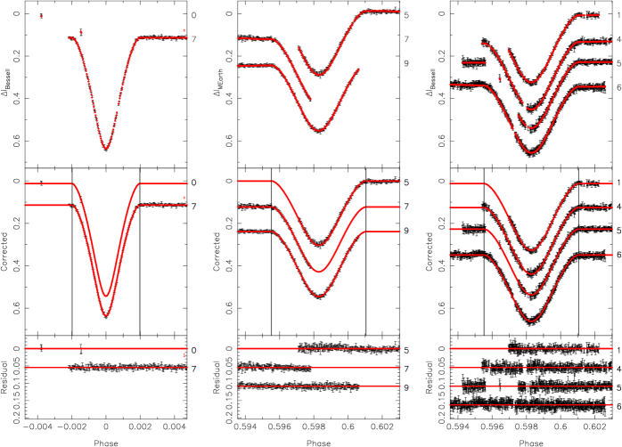
Figure 6.— Eclipse light curves used in the model, with the best fit overlaid (the model is the first of the assumptions in Table 6, but the other model light curves are almost identical in appearance). In the top panels, the model is shown with red dots at the epochs of the observations, and in the other panels it is plotted as a continuous curve. The figure has been divided horizontally into one column for each combination of eclipse and passband, with the primary eclipses (all in $I_{\rm Bessell}$) plotted on the left, the secondary eclipses in $I_{\rm MEarth}$ in the center, and in $I_{\rm Bessell}$ on the right. Each column contains three panels showing the raw differential photometry (top), the same after correction to flatten the out of eclipse baseline (center; these corrections are the airmass term for the Clay and MEarth secondary eclipses, and the “common-mode” term for the MEarth secondary eclipses) and the residual in the bottom panel. We have offset the different eclipses vertically for clarity, and the cycle number (integer part of the normalized orbital phase) is shown on the right. The vertical bars indicate the approximate locations of the first and last contact points.

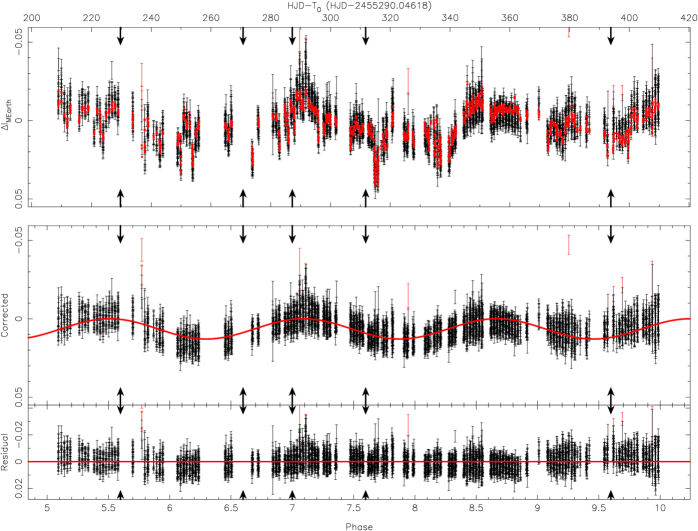
Figure 7.— MEarth 2010-2011 season out of eclipse light curve. Vertical panels as Fig. 6, with the best-fitting sinusoidal model overplotted. Arrows indicate the phases corresponding to the observed eclipses.

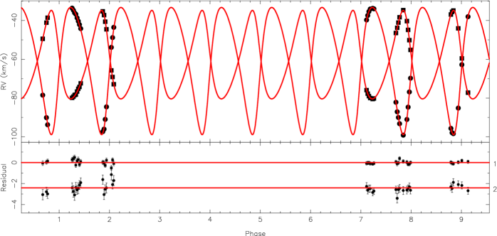
Figure 8.— Radial velocity curves used in the model, with the best fit overlaid (top) and residual (bottom). The primary velocities are shown with square symbols, and the secondary velocities with round symbols. The residuals for the two stars have been offset for clarity.

The 2010 November 19 partial secondary eclipse from MEarth (numbered $5$ in the figure) provides the most discriminating power between the various models, particularly taken in conjunction with the 2011 May 2 event (numbered $9$), which dominates the fit. As shown in Figure 7, these were taken at opposite extremes of the out of eclipse variation, with the 2010 November 19 event at maximum light and the 2011 May 2 event close to minimum light. Examining the sizes of the $s$ parameter in Table 6, the “eclipsed spots” model on the secondary, which is the only model presenting a significant detectable deviation in the secondary eclipses (as shown in Figure 5) is disfavored by the data (see Figure 9), having an $s_{\rm MEarth-20101119}$ value larger by almost $3\sigma$ than the “non-eclipsed spots” model on the secondary. Indeed, the observations indicate that this eclipse needs to be made as shallow as possible in the model in order to produce a good fit, possibly even slightly shallower than the “non-eclipsed spots” model is able to produce (the discrepancy may arise from the imperfect modeling of the out-of-eclipse variation by a sinusoid). The depth of this eclipse therefore argues that if the spots causing the out of eclipse modulation are on the secondary, they should be at latitudes not crossed by the eclipse chord.

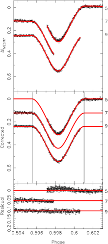
Figure 9.— As Figure 6, except for the “eclipsed spots” model on the secondary, showing the deviations in the MEarth 2010 November 19 event.

It is interesting to note that, because the radius ratio is quite close to unity, the range of allowed combinations of spot latitude and inclination angle for the secondary that would explain the observed out of eclipse modulations is therefore quite narrow, compared to the much wider range of possibilities on the primary that are still allowed. This mildly argues in favor of spots on the primary as being the more likely explanation, purely from geometry.

Nevertheless, with the presently-available data, the other models do not show any clear disagreement with the observations, so we consider (from a purely observational point of view) that all three are equally likely at present.

4.3.3 Effect of additional spots

The model we have considered so far uses the minimum spot coverage necessary to reproduce the observed out-of-eclipse modulations. As noted, e.g. by Barnes et al. (2011) and other authors, studies of cool stars sensitive to the total spot coverage typically find much higher filling factors than photometric spot models. Therefore it is likely these stars have a significant longitudinally homogeneous spot component.

In this section, we consider the effect of adding additional spots in a longitudinally homogeneous fashion where they would not be detectable through modulations in the photometry. For simplicity, we have placed these spots on the same star and at the same latitudes as the longitudinally inhomogeneous component, noting that we are predominantly interested in the effect on the component radii, where it does not matter which of the possible locations is used for the longitudinally inhomogeneous spot component.

As discussed earlier, the spectroscopic light ratio is sensitive to differences in the overall spot coverage between the two stars in some cases. We have explored this limit, and the effect of adding varying quantities of spots on the component radii, by subtracting an extra term $c_{i}$ in Eq. (3) representing the fraction of stellar light removed by the longitudinally homogeneous spot component.

For single late-type active dwarfs, it is typical to find spot filling factors of $20-50\%$ from observations sensitive to the entire surface spot coverage (e.g. O’Neal et al. 2004), although we note the available information for M-dwarfs is very limited. Photometric observations of M-dwarfs indicate spot temperature contrast of up to $10\%$ (e.g. Rockenfeller et al. 2006, who find $4-8\%$). This yields a decrement of approximately $10-20\%$ in the $I$-band stellar light, assuming parameters appropriate to the present system, with the lower end of the range presumably more typical for less active stars. We therefore consider values of $c_{i}=0.1$ and $0.2$. The latter corresponds approximately to the spot levels discussed by Morales et al. (2010) for the existing short-period eclipsing binaries. The results are given in Tables 7 and 8.

Table 7 Derived parameters and uncertainties showing the effect of additional spots on the primary.

	Non-eclipsed spots			Eclipsed spots
Parameter	$c_{1}=0$	$c_{1}=0.1$	$c_{1}=0.2$	$c_{1}=0$	$c_{1}=0.1$	$c_{1}=0.2$
$J_{\rm MEarth}$	$0.7999\pm 0.0064$	$0.8302\pm 0.0066$	$0.8724\pm 0.0074$	$0.7996\pm 0.0064$	$0.7196\pm 0.0060$	$0.6396\pm 0.0051$
$J_{\rm Bessell}$	$0.8255\pm 0.0066$	$0.8583\pm 0.0068$	$0.9042\pm 0.0079$	$0.8252\pm 0.0066$	$0.7427\pm 0.0062$	$0.6602\pm 0.0054$
$(R_{1}+R_{2})/a$	$0.015548^{+0.000039}_{-0.000042}$	$0.015632^{+0.000039}_{-0.000039}$	$0.015775^{+0.000037}_{-0.000039}$	$0.015550^{+0.000041}_{-0.000042}$	$0.015551^{+0.000042}_{-0.000044}$	$0.015550^{+0.000041}_{-0.000042}$
$R_{2}/R_{1}$	$0.787\pm 0.017$	$0.766\pm 0.016$	$0.756\pm 0.017$	$0.788\pm 0.017$	$0.788\pm 0.018$	$0.787\pm 0.017$
$\cos i$	$0.004645^{+0.000103}_{-0.000112}$	$0.005219^{+0.000083}_{-0.000086}$	$0.005861^{+0.000065}_{-0.000072}$	$0.004646^{+0.000105}_{-0.000111}$	$0.004646^{+0.000109}_{-0.000116}$	$0.004644^{+0.000107}_{-0.000112}$
$i$ (∘)	$89.7339^{+0.0064}_{-0.0059}$	$89.7010^{+0.0049}_{-0.0047}$	$89.6642^{+0.0041}_{-0.0037}$	$89.7338^{+0.0063}_{-0.0061}$	$89.7338^{+0.0067}_{-0.0063}$	$89.7339^{+0.0064}_{-0.0061}$
$L_{2}/L_{1}$	$0.485\pm 0.025$	$0.531\pm 0.025$	$0.611\pm 0.032$	$0.486\pm 0.025$	$0.486\pm 0.026$	$0.486\pm 0.025$
$(R_{1}+R_{2})$ (${\rm R}_{\odot}$)	$0.6814^{+0.0020}_{-0.0020}$	$0.6847^{+0.0020}_{-0.0020}$	$0.6904^{+0.0020}_{-0.0021}$	$0.6815^{+0.0020}_{-0.0021}$	$0.6815^{+0.0021}_{-0.0021}$	$0.6815^{+0.0020}_{-0.0021}$
$R_{1}$ (${\rm R}_{\odot}$)	$0.3815^{+0.0028}_{-0.0030}$	$0.3878^{+0.0026}_{-0.0029}$	$0.3934^{+0.0030}_{-0.0033}$	$0.3814^{+0.0028}_{-0.0031}$	$0.3814^{+0.0029}_{-0.0032}$	$0.3814^{+0.0028}_{-0.0031}$
$R_{2}$ (${\rm R}_{\odot}$)	$0.2999^{+0.0044}_{-0.0043}$	$0.2969^{+0.0042}_{-0.0039}$	$0.2970^{+0.0045}_{-0.0043}$	$0.3001^{+0.0045}_{-0.0043}$	$0.3001^{+0.0047}_{-0.0044}$	$0.3000^{+0.0045}_{-0.0043}$

Table 8 Derived parameters and uncertainties showing the effect of additional spots on the secondary.

	Non-eclipsed spots
Parameter	$c_{2}=0$	$c_{2}=0.1$	$c_{2}=0.2$
$J_{\rm MEarth}$	$0.8004\pm 0.0066$	$0.8157\pm 0.0075$	$0.8271\pm 0.0081$
$J_{\rm Bessell}$	$0.8259\pm 0.0069$	$0.8409\pm 0.0077$	$0.8516\pm 0.0084$
$(R_{1}+R_{2})/a$	$0.015551^{+0.000042}_{-0.000044}$	$0.015586^{+0.000043}_{-0.000044}$	$0.015601^{+0.000045}_{-0.000045}$
$R_{2}/R_{1}$	$0.788\pm 0.018$	$0.777\pm 0.016$	$0.757\pm 0.014$
$\cos i$	$0.00465^{+0.00011}_{-0.00012}$	$0.00493^{+0.00011}_{-0.00012}$	$0.00513^{+0.00012}_{-0.00012}$
$i$ (∘)	$89.7335^{+0.0066}_{-0.0062}$	$89.7177^{+0.0066}_{-0.0064}$	$89.7063^{+0.0067}_{-0.0066}$
$L_{2}/L_{1}$	$0.474\pm 0.025$	$0.423\pm 0.022$	$0.360\pm 0.017$
$(R_{1}+R_{2})$ (${\rm R}_{\odot}$)	$0.6815^{+0.0021}_{-0.0021}$	$0.6829^{+0.0021}_{-0.0021}$	$0.6834^{+0.0022}_{-0.0022}$
$R_{1}$ (${\rm R}_{\odot}$)	$0.3814^{+0.0028}_{-0.0032}$	$0.3844^{+0.0026}_{-0.0029}$	$0.3892^{+0.0021}_{-0.0024}$
$R_{2}$ (${\rm R}_{\odot}$)	$0.3001^{+0.0047}_{-0.0044}$	$0.2985^{+0.0044}_{-0.0042}$	$0.2942^{+0.0040}_{-0.0037}$

Firstly, it is clear from Table 7 that adding additional “eclipsed spots” has no effect on the radii or light ratio and merely alters the surface brightness ratio (this means it also changes the effective temperature ratio). This is also true when placing these spots on the secondary, but we do not show results for this model since it is unable to reproduce the observed eclipse light curves, as discussed in §4.3.2.

Adding “non-eclipsed spots” affects the light ratio, and both component radii, slightly increasing the sum of the radii, increasing $R_{1}$, and decreasing $R_{2}$. The light ratio behaves as expected, becoming closer to unity as the primary is darkened by the addition of spots. Both $c_{2}=0.2$ models with “non-eclipsed spots” (and to some extent, the $c_{2}=0.1$ model) produce a light ratio that is marginally discrepant with the spectroscopic value (see §3 or Table 5), but the other models agree reasonably well within the errors.

Given the lack of clearly-detected perturbations in the best quality eclipse curves, it is reasonable to favor the “non-eclipsed spots” models over the “eclipsed spots” models. Assuming the $c_{i}=0.1$ model is typical, and the $c_{i}=0$ and $0.2$ models represent the likely range of values, we estimate the final system parameters and their uncertainties by combining the posterior probability distributions from all six “non-eclipsed spots” models in this section (all three values of $c_{i}$). These parameters and estimated uncertainties are reported in §4.7.

4.4. Bandpass mismatch

A concern when combining light curves taken with different instruments, is the effect of any difference in the photometric bandpasses. In the present case, where the primary and secondary eclipses were (by necessity) measured using different instruments, this predominantly affects the ratio of the eclipse depths, and thus the parameter $J$, the ratio of central surface brightnesses.

In order to determine the approximate size of the bandpass mismatch, we measured the difference in magnitude between LSPM J1112+7626 and a nearby, much bluer comparison star, at $11^{h}12^{m}12^{s}.15$ $+76^{\circ}27\arcmin 33\farcs 8$ (position from 2MASS; this is the bright star seen near the upper left corner of Figure 2). The latter star has $(J-K)_{\rm 2MASS}=0.27$ and is thus probably in the F spectral class. It is non-variable at the precision of the MEarth data (rms scatter $0.003\ {\rm mag}$).

Our measured magnitude differences were $\Delta I({\rm Hankasalmi})=0.36$, $\Delta I({\rm Clay})=0.35$, and $\Delta I({\rm MEarth})=0.55$. The excellent agreement between the two $I_{\rm Bessell}$ filters (especially in light of the observed out of eclipse variations of our target) indicates they are most likely an extremely good match.

Assuming a simple linear scaling, we estimate the change in $J$ corresponding to the mismatch between the two $I_{\rm Bessell}$ filters is approximately $1/10$ of that between the $I_{\rm Bessell}$ and $I_{\rm MEarth}$ filters, or $\delta J\approx 0.003$. This is unimportant compared to the other sources of uncertainty (see Table 6).

4.5. Limb darkening

4.5.1 Differences between $I_{\rm Bessell}$ and $I_{C}$

We first examine the effect of assuming the limb darkening law is the same in the two $I$ filters. To do this, we compare the fitting results using our baseline model to using the coefficients for the $z^{\prime}$ SDSS passband from Claret (2004), where the $I_{\rm Bessell}$ band should lie inbetween these two extremes.

Using the observed colors of LSPM J1112+7626, we estimate that approximately $1/3$ the difference between the $I_{C}$ and $z^{\prime}$ results is appropriate for the error introduced by our assumption of the $I_{C}$ limb darkening law in fitting the $I_{\rm Bessell}$ data. Comparing the results for the two bands in Table 9, we find this source of error in the radii is negligible (although it does affect $J$ and $i$ at close to $1\sigma$). While the radius sum error is comparable to the individual estimated uncertainties in the table, the uncertainty in this parameter for our adopted solution combining six spot configurations is larger, and the limb darkening contribution is then less important.

Table 9 Comparison of derived parameters and uncertainties for $I_{C}$ and $z^{\prime}$ limb darkening laws using the “non-eclipsed spots” model on the primary.

Parameter	$I_{C}$	$z^{\prime}$
$J_{\rm MEarth}$	$0.7999\pm 0.0064$	$0.7829\pm 0.0085$
$J_{\rm Bessell}$	$0.8255\pm 0.0066$	$0.8073\pm 0.0091$
$(R_{1}+R_{2})/a$	$0.015548^{+0.000039}_{-0.000042}$	$0.015387^{+0.000053}_{-0.000056}$
$R_{2}/R_{1}$	$0.787\pm 0.017$	$0.773\pm 0.022$
$\cos i$	$0.00464^{+0.00010}_{-0.00011}$	$0.00440^{+0.00016}_{-0.00017}$
$i$ (∘)	$89.7339^{+0.0064}_{-0.0059}$	$89.7481^{+0.0096}_{-0.0089}$
$L_{2}/L_{1}$	$0.485\pm 0.025$	$0.462\pm 0.031$
$(R_{1}+R_{2})$ (${\rm R}_{\odot}$)	$0.6814^{+0.0020}_{-0.0020}$	$0.6744^{+0.0025}_{-0.0027}$
$R_{1}$ (${\rm R}_{\odot}$)	$0.3815^{+0.0028}_{-0.0030}$	$0.3807^{+0.0033}_{-0.0039}$
$R_{2}$ (${\rm R}_{\odot}$)	$0.2999^{+0.0044}_{-0.0043}$	$0.2938^{+0.0059}_{-0.0055}$

4.5.2 Errors in the atmosphere models

We have assumed limb darkening coefficients fixed to the theoretical values from phoenix model atmospheres throughout the analysis. We note that the same atmosphere models have issues reproducing the observed spectra of M-dwarfs in the optical, which raises the possibility of systematic errors in the limb darkening law. In the literature, this is conventionally addressed by analyzing photometry in multiple passbands, which is sensitive to differences in the limb darkening as a function of wavelength. We do not have multi-band photometry, but note this could be an important area for future work.

It has long been recognized (e.g. Nelson & Davis 1972 and references therein) that changes in the radius of the eclipsed star mimic changes in the limb darkening. In a system with near-equal stars such as the present, it is reasonable to expect any systematic error in the limb darkening from the models should affect both stars similarly, and thus to first order, the dominant effect will be on the sum of the radii (and the inclination, but any uncertainties here have negligible effect on the final parameters).

We verified this using simulations where the square root limb darkening coefficients were varied, finding a strong correlation between $(R_{1}+R_{2})/a$ and the integral of the specific intensity over the stellar disc, which is $1-u/3-u^{\prime}/5$ for the square root law (it is also correlated to a lesser extent with $J$ and $\cos i$). This quantity is the normalization term in the eclipse depths in the photometric model, so it is not surprising that it should directly influence the quantities derived from the absolute eclipse depth. This is predominantly a concern for the interpretation of the sum of the radii: we find even quite large changes in the limb darkening law do not significantly alter the individual radii compared to their uncertainties in our adopted model.

4.6. Third light

We now examine our assumption of no third light. While the proper motion evidence (see Figure 2) argues it is unlikely there are any background stars contributing at a significant level in the photometric aperture, the relatively low proper motion of our target does not allow this possibility to be completely eliminated given the limited angular resolution of the first epoch imaging data. Common proper motion companions are also permitted at intermediate separations below the angular resolution of the SDSS data, but still in wide enough orbits or with mass ratios much less than unity, where they would not be detected by the presence of additional lines in the spectra or radial velocity drift over the approximately 1 year baseline available.

Therefore, to examine any constraints on third light which can be placed directly from the light curves, and the effect on the derived parameters, we ran an additional set of Monte Carlo simulations using the basic “non-eclipsed spots” model on the primary discussed in §4.3.2 and Table 6, allowing $L_{3}$ to vary. For simplicity, a uniform prior was assumed. We find $L_{3}<0.029$ at $95\%$ confidence. As discussed by Nelson & Davis (1972), the dominant parameter mimic is between third light and inclination, and our results confirm this, finding the uncertainties in $\cos i$ and the central surface brightness ratio parameters were slightly inflated. The other light curve parameters and radii derived from these chains are indistinguishable within the uncertainties from the results where $L_{3}$ was not varied.

4.7. Summary and adopted system parameters

Of the sources of uncertainty we have considered, spots dominate. Since the stars hosting the spots and the spot configuration are mostly unknown, we adopt the union of the six spotted solutions discussed in §4.3.3, giving them equal weight. The final parameter estimates and their uncertainties are reported in Table 10, derived from the posterior samples produced by the Monte Carlo simulations, adopting the median and $68.3\%$ central confidence intervals as the central value and uncertainty (see §4.2).

Table 10 Adopted physical parameters and uncertainties, combining six spot configurations.

Parameter	Value
	C08	L96
$M_{1}$ (${\rm M}_{\odot}$)	$0.3946\pm 0.0023$
$M_{2}$ (${\rm M}_{\odot}$)	$0.2745\pm 0.0012$
$(R_{1}+R_{2})$ (${\rm R}_{\odot}$)	$0.6834^{+0.0046}_{-0.0028}$
$R_{1}$ (${\rm R}_{\odot}$)	$0.3860^{+0.0055}_{-0.0052}$
$R_{2}$ (${\rm R}_{\odot}$)	$0.2978^{+0.0049}_{-0.0046}$
$\log g_{1}$	$4.861\pm 0.012$
$\log g_{2}$	$4.929\pm 0.014$
$T_{\rm eff,1}$ (K)	$3061\pm 162$	$3191\pm 164$
$T_{\rm eff,2}$ (K)	$2952\pm 163$	$3079\pm 166$
$T_{\rm eff,2}/T_{\rm eff,1}$	$0.959^{+0.049}_{-0.025}$	$0.960^{+0.048}_{-0.025}$
$L_{\rm bol,1}$ (${\rm L}_{\odot}$)	$0.0119\pm 0.0025$	$0.0141\pm 0.0028$
$L_{\rm bol,2}$ (${\rm L}_{\odot}$)	$0.0061\pm 0.0014$	$0.0073\pm 0.0016$
$(m-M)$	$3.40\pm 0.22$	$3.53\pm 0.22$
$d$ (pc)	$48.1\pm 5.0$	$51.0\pm 5.2$
$U$ (km/s)	$56.1\pm 3.1$	$57.6\pm 3.2$
$V$ (km/s)	$-44.4\pm 1.7$	$-44.8\pm 1.8$
$W$ (km/s)	$-10.8\pm 3.2$	$-9.1\pm 3.4$

We compute UVW space motions for LSPM J1112+7626 using the method of Johnson & Soderblom (1987), with the distance from the eclipsing binary solution, $\gamma$ velocity from Table 6, and position and proper motions from Table 3. We find this object is in the old Galactic disk population, following the method and definitions in Leggett (1992).

For very precise work, even matters as seemingly trivial as physical constants can be important, so we briefly discuss our assumptions in this regard. We adopt the 2009 IAU values of $G{\rm M}_{\odot}$ and the astronomical unit (see the Astronomical Almanac 2011), and follow Cox (2000) in adopting the value of the solar photospheric radius from Brown & Christensen-Dalsgaard (1998). For the solar effective temperature, we use the value of $5781\ {\rm K}$ from Bessell et al. (1998), which is based on measurements of the solar constant by Duncan et al. (1982).

The final constant, the solar bolometric absolute magnitude, is a more thorny issue, as discussed by Bessell et al. (1998), and extensively by Torres (2010). When using tables of bolometric corrections, it is vital to adopt the consistent value of this quantity in accordance with the table. We therefore use the appropriate values in each case in the following section.

4.8. Effective temperatures, bolometric luminosities and distance

In order to estimate effective temperatures (and thus, bolometric luminosities, and the distance), an external estimate of the effective temperature of one of the binary components is required, in addition to bolometric corrections. For M-dwarfs, there are large systematic uncertainties in the effective temperature scale (e.g. Allard et al. 1997; Luhman & Rieke 1998), with disagreement at the few hundred degrees Kelvin level among different authors. Many of the early difficulties were due to the lack of model atmospheres (which are usually needed to integrate the full SED from the available measurements to obtain $L_{\rm bol}$), and significant improvement on this front was made in the 1990s. The availability of a much larger sample of angular diameter measurements from interferometry should further improve the situation as this provides a much more direct method to estimate $T_{\rm eff}$ for single stars, but there are relatively few temperature scales available at the present time using this information.

We show results from two different inversions to illustrate the typical range of parameters. Both scales we use were derived with model atmospheres rather than blackbodies, and in both cases we use the measured $I_{C}-J_{\rm 2MASS}$, $I_{C}-H_{\rm 2MASS}$ and $I_{C}-K_{\rm 2MASS}$ colors from Table 3 in conjunction with the component radii and $I_{C}$-band light ratio from the adopted eclipsing binary solution. The results from these different pairings of bandpasses were found to be consistent within the uncertainties, so we report the union of the results.

The two sets of effective temperature and bolometric corrections adopted were from Casagrande et al. (2008), which is a recent determination using interferometric angular diameter measurements to derive $T_{\rm eff}$, and from Leggett et al. (1996), which is the basis for several recent works and tabulations of the effective temperature scale, including Luhman & Rieke (1998), Luhman (1999), and Kraus & Hillenbrand (2007).

For the Leggett et al. (1996) scale, we fit polynomials to their tabulated data, omitting three objects these authors found to be metal poor from our fits: Gl 129, LHS 343, and LHS 377. We follow Leggett et al. (1996) in adopting a systematic uncertainty of $150\ {\rm K}$, which appears to be consistent with the differences we find between the two determinations.

Our results for LSPM J1112+7626 are reported in Table 10.

5. Discussion

We now compare our results for LSPM J1112+7626 with theoretical models from Baraffe et al. (1998) and other literature objects with shorter periods summarized in Table 11. We first show the conventional mass-radius diagram in Figure 10, and then the corresponding mass-effective temperature ($T_{\rm eff}$) diagram in Figure 11.

Table 11 Detached, double-lined, double-eclipsing main sequence EB components below $0.4\ {\rm M}_{\odot}$

Name	Period	$M$	$R$	$T_{\rm eff}$	$[{\rm M/H}]$	Source
	(days)	(${\rm M}_{\odot}$)	(${\rm R}_{\odot}$)	(K)
SDSS-MEB-1 A	$0.407$	$0.272\pm 0.020$	$0.268\pm 0.0090$	$3320\pm 130$	…	1
SDSS-MEB-1 B		$0.240\pm 0.022$	$0.248\pm 0.0084$	$3300\pm 130$
GJ 3236 A	$0.771$	$0.376\pm 0.016$	$0.3795\pm 0.0084$	$3312\pm 110$	…	2
GJ 3236 B		$0.281\pm 0.015$	$0.300\pm 0.015$	$3242\pm 108$
CM Dra A	$1.27$	$0.2310\pm 0.0009$	$0.2534\pm 0.0019$	$3130\pm 70$	$[-1,-0.6]$	3
CM Dra B		$0.2141\pm 0.0010$	$0.2396\pm 0.0015$	$3120\pm 70$
LP 133-373 A	$1.63$	$0.340\pm 0.014$	$0.33\pm 0.02$	$3058\pm 195$	…	4
LP 133-373 B		same	same	$3144\pm 206$	…
MG1-2056316 B	$1.72$	$0.382\pm 0.001$	$0.374\pm 0.002\pm 0.002$	$3320\pm 180$	…	5
KOI 126 B	$1.77$	$0.2413\pm 0.0030$	$0.2543\pm 0.0014$	…	$+0.15\pm 0.08$	6
KOI 126 C		$0.2127\pm 0.0026$	$0.2318\pm 0.0013$	…
CCDM J04404+3127 B,C	$2.05$	…	…	…	…	7
CU Cnc B	$2.77$	$0.3980\pm 0.0014$	$0.3908\pm 0.0094$	$3125\pm 150$	…	8
1RXS J154727.5+450803 A	$3.55$	$0.2576\pm 0.0085$	$0.2895\pm 0.0068$	…	…	9
1RXS J154727.5+450803 B		$0.2585\pm 0.0080$	same	…

Figure 10.— Mass-radius relation for components of detached, double-lined, double-eclipsing binary systems below $0.4\ {\rm M}_{\odot}$. LSPM J1112+7626 is shown as bold, black points, and the literature systems from Table 11 are shown in gray, excluding CCDM J04404+3127B,C, which does not have a full solution available at present, but including KOI 126. The lines show stellar evolution models from Baraffe et al. (1998) for $10\ {\rm Gyr}$ age, $[{\rm M/H}]=0$ (solid line), $[{\rm M/H}]=-0.5$ (dashed line), and the $[{\rm M/H}]=0$ model with the radius inflated by $5\%$, corresponding to $\rho=1.05$ (dotted line).

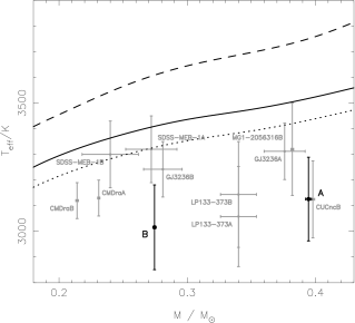
Figure 11.— Mass-effective temperature relation for components of detached, double-lined, double-eclipsing binary systems below $0.4\ {\rm M}_{\odot}$. Lines and points as Figure 10. KOI 126B,C and 1RXS J154727.5+450803 do not have reported effective temperatures, so they do not appear on this diagram. The dotted line shows the prediction from assuming $\rho=1.05$ and that the bolometric luminosity is preserved.

We also perform a quantitative comparison with the same models. We follow Torres (2007) in defining a parameter equal to the ratio of the observed radius to that predicted by the models given the observed mass, although we denote this parameter by $\rho$ instead, to avoid any potential confusion with the $\beta$ parameter defined by Chabrier et al. (2007) and used by Morales et al. (2010), which is not the same.

As argued in Torres (2007), there is evidence that the bolometric luminosities from the models are not seriously in error. If this is the case, a corresponding factor of $\rho^{-1/2}$ must be applied to the effective temperatures from the models when inflating the radii, in order to preserve the bolometric luminosity. We show results for this scenario in the tables and plots. Note, however, that the bolometric luminosity is not preserved in several recent theoretical works (Chabrier et al., 2007; Morales et al., 2010; MacDonald & Mullan, 2011), so the temperatures derived from this procedure should not be considered definitive.

As is often the case in eclipsing binaries, while the individual masses of the objects are well-determined from the radial velocities, the sum of the radii is much better determined than the individual radii, modulo limb darkening uncertainties as discussed in §4.5. We therefore compute, in addition to the $\rho$ values for the individual stars, a “composite” value comparing the model-predicted radius sum given the individual observed masses, to the measured radius sum. This quantity, which we call $\rho_{1+2}$, has much smaller formal uncertainties than the individual $\rho_{1}$ and $\rho_{2}$ values, and measures essentially a “weighted average inflation” for the whole system. These quantities, and the corresponding effective temperatures predicted from preserving the bolometric luminosity, are given for a range of assumptions for the age and metallicity in Table 12. While we caution over-interpretation of the $\rho_{1+2}$ results due to limb darkening uncertainty, the individual values should be much less prone to this problem.

Table 12 Quantitative mass-radius comparison of LSPM J1112+7626 with models.

Age	$[{\rm M/H}]$	$\rho_{1}$	$\rho_{2}$	$T_{\rm eff,1}$	$T_{\rm eff,2}$	$T_{\rm eff,2}/T_{\rm eff,1}$
(Gyr)		$\rho_{1+2}$		(K)	(K)
$1$	$0.0$	$1.054\pm 0.016$	$1.096\pm 0.018$	$3426\pm 27$	$3255\pm 26$	$0.950\pm 0.013$
$1$	$-0.5$	$1.070\pm 0.016$	$1.130\pm 0.018$	$3621\pm 28$	$3387\pm 27$	$0.935\pm 0.013$
$5$	$0.0$	$1.037\pm 0.015$	$1.072\pm 0.017$	$3453\pm 27$	$3293\pm 27$	$0.954\pm 0.013$
$5$	$-0.5$	$1.055\pm 0.016$	$1.101\pm 0.018$	$3648\pm 29$	$3436\pm 28$	$0.942\pm 0.013$
$10$	$0.0$	$1.029\pm 0.015$	$1.052\pm 0.017$	$3468\pm 27$	$3324\pm 27$	$0.959\pm 0.013$
$10$	$-0.5$	$1.047\pm 0.016$	$1.078\pm 0.017$	$3666\pm 29$	$3475\pm 28$	$0.948\pm 0.013$
$1$	$0.0$	$1.0706^{+0.0091}_{-0.0055}$		$3396\pm 13$	$3291\pm 12$	$0.96906\pm 0.00035$
$1$	$-0.5$	$1.0941^{+0.0092}_{-0.0055}$		$3579\pm 14$	$3439\pm 13$	$0.96096\pm 0.00045$
$5$	$0.0$	$1.0505^{+0.0089}_{-0.0053}$		$3428\pm 13$	$3323\pm 12$	$0.96940\pm 0.00038$
$5$	$-0.5$	$1.0735^{+0.0091}_{-0.0055}$		$3614\pm 14$	$3477\pm 13$	$0.96195\pm 0.00050$
$10$	$0.0$	$1.0378^{+0.0087}_{-0.0052}$		$3451\pm 13$	$3344\pm 12$	$0.96915\pm 0.00040$
$10$	$-0.5$	$1.0590^{+0.0091}_{-0.0056}$		$3642\pm 15$	$3504\pm 13$	$0.96221\pm 0.00052$

5.1. Mass-radius comparison

We first limit our comparisons to the mass-radius plane. If the metallicity is solar, the sum of radii is inflated at the $7\sigma$ level compared to the models, even for $10\ {\rm Gyr}$ age, which produces the largest model radii. The discrepancies are not as significant in the individual radii, with the primary $2\sigma$ and the secondary $3\sigma$ larger than the model predictions. We also note that the “eclipsed spots” model on the secondary, which we discarded in §4.3, does not solve the radius discrepancy, having a secondary radius (and sum of radii) even further from the model predictions.

Youth is unlikely as an explanation given the old disk kinematics of our target. We estimate an age of approximately $120\ {\rm Myr}$ at solar metallicity would be needed to bring the radius sum into agreement with the models, yet such objects should also rotate extremely rapidly and exhibit strong H$\alpha$ emission (e.g. Terndrup et al. 2000; Hartman et al. 2010, and references therein), neither of which are seen.

Metallicity may provide a viable explanation for the observed radii given the present uncertainties (both in the observations and the models, where for the latter it is possible the effect of metallicity on radius is underpredicted; see §1 and López-Morales 2007), although the object would most likely need to be extremely metal rich. This would place it in the tail of the metallicity distribution for the old Galactic disk population, which is likely to peak around $[{\rm M/H}]\approx-0.5$ (e.g. Leggett 1992 and references therein).

Given that metallicity has difficulty reproducing radii in other well-observed systems (see §1) and the kinematic evidence, we proceed to examine other possible causes of the inflated radii.

It is tempting to suggest that the inflation in LSPM J1112+7626 results from elevated activity levels in one or both components. While the lack of H$\alpha$ emission, unless this is rendered undetectable by the limited signal-to-noise ratio of our spectra, may be a difficulty for this scenario to explain, it should be noted that more modest levels of activity can result in weakened H$\alpha$ emission, or even absorption, but may still produce sufficient spot coverage to explain the inflation.

This system straddles (in mass) the full convection limit, where a substantial increase in the observed activity lifetimes for M-dwarfs occurs (e.g. West et al. 2008). This would argue that the secondary is more likely to be active and thus the source of the inflation. The secondary lines in the spectrum are also more difficult to observe due to its lower luminosity, which would make an H$\alpha$ line easier to hide in the noise. Identification of the star hosting the out of eclipse modulations may shed additional light on which of the components might be responsible for the inflation.

As discussed by Morales et al. (2010), the radius inflation inferred from eclipsing binary analyses often implies extremely high spot filling factors. We estimate that $\rho=1.05$ corresponds to $\beta=0.1$. Assuming a spot temperature contrast of $T_{\rm eff,spot}/T_{\rm eff,phot}=0.9$, this would require a filling factor of approximately $30\%$. This is much larger than needed to produce the observed out of eclipse modulation, and would mean there is a substantial longitudinally symmetric spot component, if the inflation is indeed caused by spots. We showed in §4.3.3 that such a level of spots does slightly modify the component radii if they are not eclipsed, reducing $R_{2}$ and increasing $R_{1}$. In practice, this may slightly reduce the required filling factor depending on where the spots are located, but unless the spot coverage is much larger than we assumed, the systematic errors in the radii resulting from such spots are still insufficient to explain the observations without invoking inflation.

Finally, on suggestion of the referee, we note that this object may indicate the need to revisit the equation of state for very low mass stars, which was discussed as a possibility to explain the radius inflation before the activity hypothesis gained prevalence (e.g. Lopez-Morales 2004; Torres & Ribas 2002). The equation of state was a significant source of difficulty in early work attempting to model very low mass stars (Chabrier & Baraffe, 1995), and although substantial progress on this front has been made (see the reviews by Chabrier & Baraffe 2000; Chabrier et al. 2005), it is still an open question.

5.2. Mass-$T_{\rm eff}$ comparison

Comparisons in only the mass-radius plane ignore important information contained in the effective temperatures. The correct physical model must explain all of the observations simultaneously, so we now proceed to examine the temperatures. This comparison is more problematic than in mass-radius for a number of reasons. The main observational issues are the difficulty of constraining effective temperatures (see §4.8) and metallicities for the eclipsing binaries.

As noted in §1, unlike the radius, the effective temperature predicted from models does depend quite strongly on metallicity, because the bolometric luminosity is a function of metallicity. As the metallicity is decreased, the model bolometric luminosity and effective temperature increase, and the radius decreases by a small amount. While metallicity does complicate the interpretation of the mass-$T_{\rm eff}$ diagram, this a key argument against metallicity as the explanation for all of the inflated radii in the eclipsing binary sample, as discussed already in §1. In this regard, CM Dra is puzzling as several authors have claimed this object is metal poor, which would further exacerbate the effective temperature discrepancy with the models.

Given the present uncertainties, it is not clear if the effective temperature difference between LSPM J1112+7626 and the models is significant. However, it does lie at the low-temperature end of the eclipsing binary results, and this lends support to the hypothesis that this object is more metal rich than the other eclipsing binaries.

5.3. Future work

It is clear that LSPM J1112+7626 offers one of the best prospects to observationally test the causes of inflated radii in eclipsing binaries, but further observations are needed. The most fruitful avenues would be to pursue a determination of the metallicity, improvement of the system parameters with a particular focus to investigating potential systematics in the radii (e.g. due to spots), and constraining the activity levels in the components by independent means (for example, X-ray emission, or the Caii H and K lines).

While we have mentioned the non-synchronized spin and orbit, we were unable to take full advantage of this property with the available observational data. As shown in §4.3, the effect of spots should be larger on the primary eclipse, so we advocate an intensive campaign on these events, preferably to obtain multiple, complete eclipses with the same telescope and detector system at a range of rotational phases and in multiple wavelengths. The primary eclipses are observable from Europe and Scandinavia during the winter 2011-2012 season, where excellent observational facilities are available. We remind observers that good-quality out of eclipse monitoring will be important for the interpretation of the eclipses themselves, and the spot distributions are likely to evolve (indeed, Figure 7 indicates that we may have already seen this in the existing data), so the monitoring must be contemporaneous, and preferably also taken at multiple wavelengths to constrain the spot temperatures.

References

- Abazajian et al. (2009) Abazajian, K. N., et al. 2009, ApJS, 182, 543
- Allard et al. (1997) Allard, F., Hauschildt, P. H., Alexander, D. R., & Starrfield, S. 1997, ARA&A, 35, 137
- Andersen (1991) Andersen, J. 1991, A&A Rev., 3, 91
- Baraffe et al. (1998) Baraffe, I., Chabrier, G., Allard, F., & Hauschildt, P. H. 1998, A&A, 337, 403
- Barnard (1916) Barnard, E. E. 1916, AJ, 29, 181
- Barnes & Collier Cameron (2001) Barnes, J. R., & Collier Cameron, A. 2001, MNRAS, 326, 950
- Barnes et al. (2004) Barnes, J. R., James, D. J., & Collier Cameron, A. 2004, MNRAS, 352, 589
- Barnes et al. (2011) Barnes, J. R., Jeffers, S. V., & Jones, H. R. A. 2011, MNRAS, 412, 1599
- Bean et al. (2006) Bean, J. L., Sneden, C., Hauschildt, P. H., Johns-Krull, C. M., & Benedict, G. F. 2006, ApJ, 652, 1604
- Benedict et al. (1998) Benedict, G. F., et al. 1998, AJ, 116, 429
- Berger et al. (2006) Berger, D. H., et al. 2006, ApJ, 644, 475
- Berta et al. (2011) Berta, Z. K., Charbonneau, D., Bean, J., Irwin, J., Burke, C. J., Désert, J.-M., Nutzman, P., & Falco, E. E. 2011, ApJ, 736, 12
- Bessel (1990) Bessel, M. S. 1990, A&AS, 83, 357
- Bessell (1990) Bessell, M. S. 1990, PASP, 102, 1181
- Bessell et al. (1998) Bessell, M. S., Castelli, F., & Plez, B. 1998, A&A, 333, 231
- Blake et al. (2008) Blake, C. H., Torres, G., Bloom, J. S., & Gaudi, B. S. 2008, ApJ, 684, 635
- Bonfils et al. (2005) Bonfils, X., Delfosse, X., Udry, S., Santos, N. C., Forveille, T., & Ségransan, D. 2005, A&A, 442, 635
- Boyajian et al. (2011) Boyajian, T. S., et al. 2011, in Cool Stars, Stellar Systems and the Sun XVI, ed. C. Johns-Krull, A. West, & M. Browning, Astronomical Society of the Pacific Conference Series, in press (arXiv:1012.0542)
- Brown & Christensen-Dalsgaard (1998) Brown, T. M., & Christensen-Dalsgaard, J. 1998, ApJ, 500, L195+
- Buchhave et al. (2010) Buchhave, L. A., et al. 2010, ApJ, 720, 1118
- Carney et al. (1989) Carney, B. W., Latham, D. W., & Laird, J. B. 1989, AJ, 97, 423
- Carter et al. (2011) Carter, J. A., et al. 2011, Science, 331, 562
- Casagrande et al. (2008) Casagrande, L., Flynn, C., & Bessell, M. 2008, MNRAS, 389, 585
- Chabrier & Baraffe (1995) Chabrier, G., & Baraffe, I. 1995, ApJ, 451, L29+
- Chabrier & Baraffe (1997) —. 1997, A&A, 327, 1039
- Chabrier & Baraffe (2000) —. 2000, ARA&A, 38, 337
- Chabrier et al. (2005) Chabrier, G., Baraffe, I., Allard, F., & Hauschildt, P. H. 2005, in Resolved Stellar Populations, ed. D. Valls-Gabaud, & M. Chavez, Astronomical Society of the Pacific Conference Series, in press (astro-ph/0509798)
- Chabrier et al. (2007) Chabrier, G., Gallardo, J., & Baraffe, I. 2007, A&A, 472, L17
- Claret (2000) Claret, A. 2000, A&A, 363, 1081
- Claret (2004) —. 2004, A&A, 428, 1001
- Coughlin et al. (2011) Coughlin, J. L., López-Morales, M., Harrison, T. E., Ule, N., & Hoffman, D. I. 2011, AJ, 141, 78
- Covey et al. (2007) Covey, K. R., et al. 2007, AJ, 134, 2398
- Cox (2000) Cox, A. N., ed. 2000, Allen’s astrophysical quantities, 4th edn. (New York: AIP Press; Berlin: Springer)
- Delfosse et al. (2000) Delfosse, X., Forveille, T., Ségransan, D., Beuzit, J.-L., Udry, S., Perrier, C., & Mayor, M. 2000, A&A, 364, 217
- Delfosse et al. (1999) Delfosse, X., Forveille, T., Udry, S., Beuzit, J., Mayor, M., & Perrier, C. 1999, A&A, 350, L39
- Demory et al. (2009) Demory, B.-O., et al. 2009, A&A, 505, 205
- Devor et al. (2008) Devor, J., et al. 2008, ApJ, 687, 1253
- Diaz-Cordoves & Gimenez (1992) Diaz-Cordoves, J., & Gimenez, A. 1992, A&A, 259, 227
- Doi et al. (2010) Doi, M., et al. 2010, AJ, 139, 1628
- Duncan et al. (1982) Duncan, C. H., Willson, R. C., Kendall, J. M., Harrison, R. G., & Hickey, J. R. 1982, Solar Energy, 28, 385
- Eggen & Sandage (1967) Eggen, O. J., & Sandage, A. 1967, ApJ, 148, 911
- Fabricant et al. (1998) Fabricant, D., Cheimets, P., Caldwell, N., & Geary, J. 1998, PASP, 110, 79
- Ford (2005) Ford, E. B. 2005, AJ, 129, 1706
- Ford (2006) —. 2006, ApJ, 642, 505
- Gizis (1997) Gizis, J. E. 1997, AJ, 113, 806
- Gizis et al. (2002) Gizis, J. E., Reid, I. N., & Hawley, S. L. 2002, AJ, 123, 3356
- Gregory (2005) Gregory, P. C. 2005, ApJ, 631, 1198
- Griffin et al. (1976) Griffin, R. F., Radford, G. A., Harmer, D. L., & Stickland, D. J. 1976, The Observatory, 96, 153
- Haario et al. (2001) Haario, P. C., Saksman, E., & Tamminen, J. 2001, Bernoulli, 7, 223
- Hartman et al. (2010) Hartman, J. D., Bakos, G. Á., Kovács, G., & Noyes, R. W. 2010, MNRAS, 408, 475
- Hartman et al. (2011) Hartman, J. D., Bakos, G. Á., Noyes, R. W., Sipőcz, B., Kovács, G., Mazeh, T., Shporer, A., & Pál, A. 2011, AJ, 141, 166
- Hewett et al. (1985) Hewett, P. C., Irwin, M. J., Bunclark, P., Bridgeland, M. T., Kibblewhite, E. J., He, X. T., & Smith, M. G. 1985, MNRAS, 213, 971
- Horne (1986) Horne, K. 1986, PASP, 98, 609
- Irwin et al. (2011) Irwin, J., Berta, Z. K., Burke, C. J., Charbonneau, D., Nutzman, P., West, A. A., & Falco, E. E. 2011, ApJ, 727, 56
- Irwin et al. (2009a) Irwin, J., Charbonneau, D., Nutzman, P., & Falco, E. 2009a, in IAU Symposium, Vol. 253, IAU Symposium, 37–43
- Irwin et al. (2007) Irwin, J., Irwin, M., Aigrain, S., Hodgkin, S., Hebb, L., & Moraux, E. 2007, MNRAS, 375, 1449
- Irwin et al. (2009b) Irwin, J., et al. 2009b, ApJ, 701, 1436
- Johnson & Soderblom (1987) Johnson, D. R. H., & Soderblom, D. R. 1987, AJ, 93, 864
- Kirkpatrick et al. (1991) Kirkpatrick, J. D., Henry, T. J., & McCarthy, Jr., D. W. 1991, ApJS, 77, 417
- Kraus & Hillenbrand (2007) Kraus, A. L., & Hillenbrand, L. A. 2007, AJ, 134, 2340
- Kraus et al. (2011) Kraus, A. L., Tucker, R. A., Thompson, M. I., Craine, E. R., & Hillenbrand, L. A. 2011, ApJ, 728, 48
- Kwee & van Woerden (1956) Kwee, K. K., & van Woerden, H. 1956, Bull. Astron. Inst. Netherlands, 12, 327
- Lacy (1977) Lacy, C. H. 1977, ApJ, 218, 444
- Landolt (1992) Landolt, A. U. 1992, AJ, 104, 340
- Leggett (1992) Leggett, S. K. 1992, ApJS, 82, 351
- Leggett et al. (1996) Leggett, S. K., Allard, F., Berriman, G., Dahn, C. C., & Hauschildt, P. H. 1996, ApJS, 104, 117
- Lépine & Shara (2005) Lépine, S., & Shara, M. M. 2005, AJ, 129, 1483
- Lopez-Morales (2004) Lopez-Morales, M. 2004, PhD thesis, The University of North Carolina at Chapel Hill
- López-Morales (2007) López-Morales, M. 2007, ApJ, 660, 732
- López-Morales & Ribas (2005) López-Morales, M., & Ribas, I. 2005, ApJ, 631, 1120
- Lucy (1967) Lucy, L. B. 1967, ZAp, 65, 89
- Luhman (1999) Luhman, K. L. 1999, ApJ, 525, 466
- Luhman & Rieke (1998) Luhman, K. L., & Rieke, G. H. 1998, ApJ, 497, 354
- MacDonald & Mullan (2011) MacDonald, J., & Mullan, D. J. 2011, ApJ, submitted (arXiv:1106.1452)
- Metcalfe et al. (1996) Metcalfe, T. S., Mathieu, R. D., Latham, D. W., & Torres, G. 1996, ApJ, 456, 356
- Morales et al. (2010) Morales, J. C., Gallardo, J., Ribas, I., Jordi, C., Baraffe, I., & Chabrier, G. 2010, ApJ, 718, 502
- Morales et al. (2009) Morales, J. C., et al. 2009, ApJ, 691, 1400
- Mullan & MacDonald (2001) Mullan, D. J., & MacDonald, J. 2001, ApJ, 559, 353
- Nelson & Davis (1972) Nelson, B., & Davis, W. D. 1972, ApJ, 174, 617
- Nutzman & Charbonneau (2008) Nutzman, P., & Charbonneau, D. 2008, PASP, 120, 317
- O’Neal et al. (2004) O’Neal, D., Neff, J. E., Saar, S. H., & Cuntz, M. 2004, AJ, 128, 1802
- Popper & Etzel (1981) Popper, D. M., & Etzel, P. B. 1981, AJ, 86, 102
- Prša et al. (2011) Prša, A., et al. 2011, AJ, 141, 83
- Reid et al. (1995) Reid, I. N., Hawley, S. L., & Gizis, J. E. 1995, AJ, 110, 1838
- Ribas (2003) Ribas, I. 2003, A&A, 398, 239
- Ribas (2006) —. 2006, Ap&SS, 304, 89
- Rockenfeller et al. (2006) Rockenfeller, B., Bailer-Jones, C. A. L., & Mundt, R. 2006, A&A, 448, 1111
- Rodono et al. (1986) Rodono, M., et al. 1986, A&A, 165, 135
- Shkolnik et al. (2010) Shkolnik, E. L., Hebb, L., Liu, M. C., Reid, I. N., & Collier Cameron, A. 2010, ApJ, 716, 1522
- Southworth et al. (2004a) Southworth, J., Maxted, P. F. L., & Smalley, B. 2004a, MNRAS, 351, 1277
- Southworth et al. (2004b) Southworth, J., Zucker, S., Maxted, P. F. L., & Smalley, B. 2004b, MNRAS, 355, 986
- Tegmark et al. (2004) Tegmark, M., et al. 2004, Phys. Rev. D, 69, 103501
- Terndrup et al. (2000) Terndrup, D. M., Stauffer, J. R., Pinsonneault, M. H., Sills, A., Yuan, Y., Jones, B. F., Fischer, D., & Krishnamurthi, A. 2000, AJ, 119, 1303
- Tody (1993) Tody, D. 1993, in Astronomical Society of the Pacific Conference Series, Vol. 52, Astronomical Data Analysis Software and Systems II, ed. R. J. Hanisch, R. J. V. Brissenden, & J. Barnes (San Francisco: ASP), 173–+
- Torres (2007) Torres, G. 2007, ApJ, 671, L65
- Torres (2010) —. 2010, AJ, 140, 1158
- Torres et al. (2010) Torres, G., Andersen, J., & Giménez, A. 2010, A&A Rev., 18, 67
- Torres & Ribas (2002) Torres, G., & Ribas, I. 2002, ApJ, 567, 1140
- Vaccaro et al. (2007) Vaccaro, T. R., Rudkin, M., Kawka, A., Vennes, S., Oswalt, T. D., Silver, I., Wood, M., & Smith, J. A. 2007, ApJ, 661, 1112
- van Hamme (1993) van Hamme, W. 1993, AJ, 106, 2096
- Viti et al. (2002) Viti, S., Jones, H. R. A., Maxted, P., & Tennyson, J. 2002, MNRAS, 329, 290
- Viti et al. (1997) Viti, S., Jones, H. R. A., Schweitzer, A., Allard, F., Hauschildt, P. H., Tennyson, J., Miller, S., & Longmore, A. J. 1997, MNRAS, 291, 780
- West et al. (2008) West, A. A., Hawley, S. L., Bochanski, J. J., Covey, K. R., Reid, I. N., Dhital, S., Hilton, E. J., & Masuda, M. 2008, AJ, 135, 785
- West et al. (2005) West, A. A., Walkowicz, L. M., & Hawley, S. L. 2005, PASP, 117, 706
- Wilson & Devinney (1971) Wilson, R. E., & Devinney, E. J. 1971, ApJ, 166, 605
- Woolf & Wallerstein (2006) Woolf, V. M., & Wallerstein, G. 2006, PASP, 118, 218
- Zahn (1977) Zahn, J. 1977, A&A, 57, 383
- Zucker & Mazeh (1994) Zucker, S., & Mazeh, T. 1994, ApJ, 420, 806