Correlating the interstellar magnetic field with protostellar jets and its sources

Abstract

This article combines new CCD polarimetric data with previous information about protostellar objects in a search for correlations involving the interstellar magnetic field. Specifically, we carried out an optical polarimetric study of a sample of 28 fields of 10′ $\times$ 10′ located in the neighborhood of protostellar jets and randomly spread over the Galaxy. The polarimetry of a large number of field stars is used to estimate both the average and dispersion of the interstellar magnetic field (ISMF) direction in each region. The results of the applied statistical tests are as follows. Concerning the alignment between the jet direction and the interstellar magnetic field, the whole sample does not show alignment. There is, however, a statistically significant alignment for objects of Classes 0 and I. Regarding the interstellar magnetic field dispersion, our sample presents values slightly larger for regions containing T Tauri objects than for those harboring younger protostars. Moreover the ISMF dispersion in regions containing high-mass objects tends to be larger than in those including only low-mass protostars. In our sample, the mean interstellar polarization as a function of the average interstellar extinction in a region reaches a maximum value around 3% for A(V) = 5, after which it decreases. Our data also show a clear correlation of the mean value of the interstellar polarization with the dispersion of the interstellar magnetic field: the larger the dispersion, the smaller the polarization. Based on a comparison of our and previous results, we suggest that the dispersion in regions forming stars is larger than in quiescent regions.

1 Introduction

The role of the magnetic field (MF) in the star formation process is an active area of research. The MF can act in phenomena at large scales, such as the collapse of a molecular cloud (e.g., Shu et al., 1987), and at smaller scales, such as the formation of protostellar jets and outflows (e.g., Ferreira et al., 2006) and disk viscosity (e.g., Königl & Salmeron, 2010). An important present question is if the interstellar magnetic field (ISMF) (e.g., Mouschovias & Ciolek, 1999; Mouschovias & Tassis, 2010) or the turbulence (e.g., McKee & Ostriker, 2007; Crutcher et al., 2009) is the main agent of the support of molecular clouds against the gravitational force.

An indication to the importance of the interstellar magnetic field (ISMF) in the collapse is the alignment between the magnetic field at larger scales and the symmetry axis of the young stellar object (YSO). The ambipolar diffusion model predicts that the collapse of the protostellar object occurs preferentially along the field lines. This results in an alignment of the ISMF with respect to the accretion disk axis (Shu et al., 1987). Simulations of the collapse of magnetized regions that forms the cores also indicate that, in plausible interstellar physical conditions, there will be an alignment. Machida et al. (2006) show that the disk axis evolves to a configuration parallel to the ISMF if the rotation rate is small relative to the ISMF strength. The simulations of Matsumoto et al. (2006) result in an alignment of the jet direction with the ISMF, if the ISMF is larger than 80 $\mu$G. Recently, turbulence has been included in those simulations (Matsumoto & Hanawa, 2011). They have found that the shape of the core depends on its mass: massive cores are prolate and low-mass cores are oblate. And, in any case, the minor axis is parallel to the ISMF.

From an observational perspective, early studies pointed to an alignment between the symmetry axis of the protostellar object and the ISMF. Dyck & Lonsdale (1979) and Heckert & Zeilik (1981) obtained near-infrared (NIR) polarimetry of compact IR sources (52 in total) and found a tendency of alignment between the circumstellar polarization and the ISMF direction. Tamura & Sato (1989), also based on NIR polarization, found similar results with a sample of 39 T Tauri objects. Snell et al. (1980) and Cohen et al. (1984) suggested an alignment between YSO outflow and ISMF. These results were later confirmed by Strom et al. (1986) using a larger sample, including 38 regions.

Recently, there has been a revival of this subject. Ménard & Duchêne (2004), using a sample composed of T Tauri stars, did not find any correlation between the YSO disk axis and the ISMF, but suggested that the brighter jets are aligned to the ISMF. Subsequent studies indicate that different interstellar structures are oriented according to the ISMF, independently of presenting or not signs of star formation. The Pipe Nebula and Musca Cloud have their long axis perpendicular to the ISMF (Franco et al. 2010 and Pereyra & Magalhães 2004, respectively). The same occurs in the Serpens Cloud (Sugitani et al., 2011). Li et al. (2009) also found that the magnetic field direction in the intercloud medium correlates with the field direction of the dense cores. Anathpindika & Whitworth (2008) studied the alignment of outflows and the filaments containing the associated dense core in a sample of 45 objects and found that the directions are approximately orthogonal. Rodrigues et al. (2009), based on a sample of 100 Herbig Ae/Be stars, suggested that the most polarized objects tend to have their polarization position angle aligned with the ISMF direction. In fact, there is evidence that the ISMF is dynamically dominant in interstellar clouds as Pipe and Serpens (Franco et al. 2010 and Sugitani et al. 2010, respectively).

Besides its direction, another property of the ISMF that can be used to understand the interstellar medium conditions is how ordered it is. Assuming the equilibrium between kinetic and magnetic forces and isotropy of the motions in the ISM, Chandrasekhar & Fermi (1953, CF53) proposed the following relation between the dispersion of ISMF direction, $\sigma_{B}$, and the 3D turbulent velocity, $\sigma(v)$:

$$\sigma_{B}=\left(\frac{4}{3}\pi\rho\right)^{\frac{1}{2}}\frac{\sigma(v)}{B},$$ (1)

where $\rho$ is the mean mass density of the interstellar medium (ISM) and $B$ is the intensity of the interstellar magnetic field.

But this simple relation has some caveats. Examples are: large fluctuations of the magnetic field amplitude; acting of the nonmagnetic forces on the gas; inhomogeneity of the interstellar material (Zweibel, 1996). Even so, numerical simulations of polarimetric maps of molecular clouds indicate that the CF53’s relation is valid at least as an order of magnitude estimate (Ostriker et al., 2001; Padoan et al., 2001; Heitsch et al., 2001).

As ISMF dispersion and turbulence are connected, we cite some recent studies on the origin of the interstellar turbulence, which are not yet conclusive. Some authors, based on simulations, suggested that stellar outflows can replenish the turbulent motion in dense cores (Nakamura & Li, 2007; Carroll et al., 2009, 2010). From an observational perspective, this scenario seems to be true in the Serpens cloud, in which the outflows have enough energy to power the observed turbulence (Sugitani et al., 2010). On the other hand, others authors, based on simulations and observations, show that the turbulence is injected in the molecular clouds by a large-scale process (Brunt et al., 2009; Padoan et al., 2009). A third different view is that in which the dispersion of the velocity is the result of gravitational collapse (Heitsch et al., 2009).

In this paper, we present a search for connections between the properties of the interstellar magnetic field and the stellar formation to constrain the magnetic field role in the star formation process. The ISMF is probed through optical polarimetry. Our observational technique allows the measurement of the polarization of a large number of objects in a region. It improves the statistical significance of our results, compared with previous studies based on photoelectric measurements, and enables the estimate of the ISMF dispersion, a quantity that is poorly explored previously due to the lack of enough data. The regions in which we sample the ISMF are spread over many molecular clouds throughout the Galaxy. This should result in unbiased results valid in the context of star formation in the Galaxy, not specific for a given star formation complex. Moreover, our fields of view are small, so more plausibly associated with the interstellar medium nearby the YSO.

This article is organized as follows. Section 2 describes the procedure of data acquisition and reduction as well as how both the average and the dispersion of the interstellar magnetic field direction are estimated. The YSO information is compiled from the literature as explained in Section 3. The statistical analysis and discussion are presented in Section 4. Our conclusions are summarized in the last section. This paper is the result of the Master dissertation of C. Targon (2008).

2 Polarization measurements and estimation of the properties of the interstellar magnetic field

We obtained the optical polarimetry of 28 southern regions close to Herbig-Haro (HH) objects from the Reipurth’s catalog (Reipurth, 1994). We randomly selected among the richer stellar fields, since the richer the field the better the mapping of the ISMF. Each region covers a sky area of 10$\farcm$5 $\times$ 10$\farcm$5. The total number of HH objects found in a radius of 20′ from the center of each field is 82, considering all fields. However, a jet can be associated with more than one HH object. Furthermore, a YSO can have a jet and its counterjet. Hence, we considered as one object the group of HHs associated with a given protostellar source (jet and counterjet). In doing this, the final number of objects (= jets, hereafter) in our data is 60. To help the reader to relate the fields to the sites of star formation, Table 1 displays a non-uniform identification of the region, cloud, or globule in the direction of each line-of-sight.

The observations were carried out in 1998 December 18, between 2005 February 11 and 17, and on 2007 May 7, with the 0.60-m Boller & Chivens telescope at the Observatório do Pico dos Dias, Brazil, operated by the Laboratório Nacional de Astrofísica, Brazil. A CCD camera modified by the polarimetric module described in Magalhães et al. (1996) has been used. The CCD array used was a SITe back-illuminated, $1024\times 1024$ pixels. This results in a field-of-view of 10$\farcm$5 $\times$ 10$\farcm$5 (1 pixel = 0$\farcs$62). All the fields were observed with a $R_{C}$ filter. The employed technique automatically eliminates the sky polarization (Piirola, 1973). Polarimetric standards stars (Serkowski et al., 1975; Bastien et al., 1988; Turnshek et al., 1990) were observed to calibrate the system and to estimate the instrumental polarization. The measured values of the unpolarized standard stars are consistent with zero within the errors. Table 2 presents a log of the observations.

The reduction was carried out using the IRAF facility. The first step in the reduction process consists of CCD imaging correction: bias and flat-field. Then, aperture photometry of the ordinary and extraordinary images of each object is performed. The resulting counts are used to calculate the polarization using the method described in Magalhães et al. (1984). For the polarimetric analysis, the package PCCDPACK (Pereyra, 2000) was used.

Our aim is to obtain the interstellar polarization of as many objects in the field as possible. The position angle of the polarization, $\theta$, is assumed to be the direction of the ISMF as projected in the plane of sky. The following analysis is based on the objects with good signal-to-noise ratio. Specifically, we have selected those with $P/\sigma_{P}\geq 3$ and this provides a maximum error on the position angle of 10°. The only exception is Field 19, including HH 160, for which we used $P/\sigma_{P}\geq 2.5$. The number of objects considered in each field, $N_{f}$, can be found in Table 3: it runs from 14 to 559. A polarimetric catalog of each field is made available as a online-only table. Table 4 shows an example of this catalog.

For each field, we constructed histograms of $\theta$. For most fields (23/28), this histogram has a very well defined Gaussian shape. In these cases, it is straightforward to estimate the average and dispersion of the direction of the ISMF from a Gaussian fit. Figure 1 shows our polarization vectors superposed on a DSS image in the line-of-sight of HH 139 (Field 17) and the corresponding histogram of the position angle of the polarization. The graphs for the other fields can be found as online-only material. Exceptions are the graphs for Fields 02 and 15, which are presented in Hickel (2002) and Rodrigues et al. (2007), respectively. Table 3 summarizes the interstellar polarimetric characteristics of each field. It lists, per field, the number of objects ($N_{f}$), the position of the peaks in the histogram of $\theta$ ($\theta_{P}$), the value adopted for the direction of the ISMF ($\theta_{B}$) and its dispersion ($\sigma_{B}$), and the average of the polarization modulus ($P_{ISM}$). The dispersion is unbiased from the mean error of the position angle as suggested by Pereyra & Magalhães (2007). The Gaussian curves depicted in the figures use the unbiased value of the dispersion.

Five fields do not show a histogram with a clear Gaussian shape: they have two peaks. In these cases, more elaborated procedures were performed to estimate the properties of ISMF direction, which are described in the following paragraphs.

Field 15 (HH135/HH136) was studied by Rodrigues et al. (2007). Here we summarize their procedure to estimate the ISMF properties in the star forming region because it was used in other fields of this study. In this region, there are two peaks in the histogram of $\theta$. Each peak is associated with objects having different mean values of polarization. In addition, the most polarized objects are fainter than those having the smallest polarizations. These two facts can be explained if the stars in this field-of-view, and hence in the histogram, come from two populations. Furthermore, we can assume that the faintest objects are also the furthest ones. Consequently one population, associated with the nearest stars, is polarized by a single interstellar cloud. The second population, including the furthest objects, is polarized by two interstellar clouds, one of which is responsible for the polarization of the first population. As the HH objects in this line-of-sight are around 3 kpc, we assumed that the more distant dust cloud is associated with the star forming region. Thus, to obtain the direction of the polarization produced in that region, the average polarization of the population which has the brighter stars was calculated and then this value was vectorially subtracted from the polarization of the population including the fainter objects (associated with the star forming region).

Fields 16 and 28, similarly to the Field 15, shows two peaks in the histogram of $\theta$ which are associated with different values of polarization. One of the peaks is composed of a small number of objects which are also the less polarized. We assumed that these objects constitute a foreground polarization component; therefore, we have adopted the same procedure as for Field 15.

In Field 13 (HH 120), the two peaks do not have different values of polarization. They are, however, spatially segregated. To represent the direction of the ISMF, we chose the value of $\theta_{P}$ corresponding to objects near HH 120.

Field 19 (HH 160) has two peaks and a small number of objects. Therefore it is difficult to perform an appropriated statistical analysis. We used the value of the dominant (in number) component.

Three fields (5, 13, and 18) have been observed with two different exposure times, $t_{exp}$, to check if the observed distribution of $\theta$ depends on how deep the image is. For the three fields, the displacement in the peak position, $\theta_{P}$, between the polarimetry using different $t_{exp}$ is negligible ($<$ 2°). For the analysis, we adopted the values obtained with the larger $t_{exp}$, which are presented in Table 3.

There are two measurements of Fields 12 and 24, which were carried out in two adjacent lines of sight (denoted by A and B) to verify if the distribution of the ISMF direction can change in the scales of the projected angular distance of an image. Notice that the sizes of the jets in these two fields are very different. While Field 24A contains HH 271-272 and the associated YSO (hence the entire jet extension), Fields 12A and 12B map the region of HH 90-92 and 597-598, a giant jet (Bally et al., 2002), which is much larger than both fields together. The results for these two cases are discussed below.

Fields 24A and 24B have similar distributions of $\theta$. Therefore we have assumed that they both trace the same ISMF distribution, and hence we have combined the two fields to obtain the values of $\theta_{B}$ and $\sigma_{B}$ used in the analysis. These values are presented in Table 3 (24AB). This table also presents the values for the individual fields for comparison.

The jet associated with HH 90-92 and HH 597-598 extends for approximately 25′ (Bally et al., 2002). An image has a side of 10′. Field 12A includes the mid portion of the jet (HH 90) and Field 12B is displaced in a direction perpendicular to the jet axis. The distribution of $\theta$ in each field is composed of an single component, but with $\theta_{P}$ differing by 70°. For the following analysis, we have adopted the values from field 12A, because it includes the jet, but we have kept the values of field 12B in Table 3 for comparison. Jets as large as the one associated with HH 90 do not dominate our sample: only 8 jets (out of 54) have extensions larger than 5′. The extension is the distance from the YSO to the end of the jet. The number 54 corresponds to the jets which has an estimate for their extension. See Section 3 and Table Correlating the interstellar magnetic field with protostellar jets and its sources for the extension of jets used here.

The distances of the HHs in our sample range from 130 to 4300 pc (see Section 3 and Table Correlating the interstellar magnetic field with protostellar jets and its sources). Consequently, our images map regions on the plane of sky extending from 0.38 pc (slightly larger than a dense core) to 12.5 pc (dimension associated with molecular clouds). The average HH distance in our sample is 750 pc, which matches to an image size of 2.2 pc. We remind the reader that the objects included in an image are from a 3D conical structure and, therefore, sample regions of different sizes depending on the distance.

3 Compiled information about the Herbig-Haro objects and its sources

We compiled some properties of the 60 jets of this work from the literature. We collected the distance, extension and position angle of the jet (Table Correlating the interstellar magnetic field with protostellar jets and its sources) and the name, luminosity, mass, and class of the associated YSO (Table Correlating the interstellar magnetic field with protostellar jets and its sources). We could not find estimates for all the above properties for some objects. We did not include the jets associated with HH 273, HH 731 and HH 735-736 in the analysis due to the lack of information in the literature. Consequently, our analysis is restricted to 57 jets. In the following paragraphs, some remarks about the compilation are given.

We used the position angle of the jet (PA) as projected in the plane of sky and in the range 0–180°. For some jets, this value can be directly read from previous articles. For the others, we estimated it using the coordinates of the HH knots and YSO or the image itself. When there is more than one value of PA (for jet and counter-jet, for instance), we use the average. Whenever possible, we crosschecked information found in the literature. In doing so, we found an inconsistency between the jet directions cited by Ray & Eisloeffel (1994) for HH 140-143 and those calculated by us using the knots coordinates presented in the same article. Our analysis indicates that there is probably an error in the knots coordinates. Hence we propose new values, which are given in Table 7.

The projected value of the jet extensions were directly collected from the literature or estimated using available data. We define the jet extension as the distance from the YSO to the jet extremity. Consequently if the literature quotes the distance between the jet and counterjet extremities, we use half this number. In some cases, the extension was derived using the angular size of the jet and the object distance. In cases in which there is more than one estimate for the distance, we used the smallest value. This is justified by the fact that the sample is biased towards smaller extensions, since (1) we use projected lengths and (2) the farthest jet point can be missed. Among the extensions collected in the literature, the only inconsistency found is for HH 444-447. The extensions presented by Reipurth et al. (1998) are correct, and not those from Mader et al. (1999). If the angle with the line of sight is known, what is true for some jets, we could derive the real jet extensions. However, only a part of our sample has this information. Hence, to keep a homogeneous procedure for all jets, we considered the length as seen projected in the plane of sky.

Concerning mass classification, we simply adopt the same qualitative classification found in the literature among low, intermediate, and high mass. HH 160 (M = 2-3 M_⊙) and HH-217 (Sp: F0-G0) were both considered as intermediate mass. The objects classified as T Tauri were considered as low-mass objects.

Some remarks about the adopted classes should be done. The objects classified in previous articles just as T Tauri stars were considered as Class II. The source of the jet associated with HH 55 seems to be a very evolved object (Graham & Chen, 1994). Hence we have considered this object as a Class II/III. In fact, it is the only possible Class III object in the sample. Our sample includes some FU Ori variables, which are probably in a transition phase from Class I to Class II (Hartmann & Kenyon, 1996).

4 Statistical analysis and discussion

This section presents the analysis of the ISMF direction and its dispersion estimated from our optical polarimetric data. Our main aim is to verify if there are statistically significant correlations between the properties of the ISMF and those of the HH and its associated YSO. This section also contains the discussion of our results.

Our statistical analysis is performed using non-parametric tests of cumulative histograms. We have used the Kolmogorov-Smirnov test (e.g., Press et al., 1986) and the Kuiper test (e.g., Press et al., 1986; Paltani, 2004). From hereafter, these tests will be called KS and Kp, respectively. Both tests compare two cumulative distributions, but each test uses a distinct quantity (statistic) to measure how different the distributions are. The statistic of the KS test is the maximum value of the absolute difference between the two distributions. The Kp test uses the sum of the absolute values of negative and positive differences and, hence, is more sensitive to differences in the entire abscissa range. Additionally, the Kp test is more appropriate for cyclic quantities. We will call the tests between a given data distribution and a uniform one KS1 and Kp1. The tests between two data distributions will be denoted as KS2 and Kp2.

The results relative to the ISMF direction are presented in Section 4.1. Section 4.2 contains the study of the ISMF dispersion. Our findings about the average polarization in the fields are shown in Section 4.3.

4.1 The alignment between the jet and the interstellar magnetic field

To measure the alignment of a jet with the ISMF, we define $\Delta\theta$: the difference between the position angle of the jet and the direction of the interstellar magnetic field. Its value is defined in the range $0-90$° because we compare directions, not senses. To study $\Delta\theta$, the Kp test is more appropriate than the KS test because $\Delta\theta$ is a cyclic quantity. Hence, in the graphs only the probability associated with the Kp test is shown. In spite of that, we have quoted, throughout the text, the probabilities associated with both tests. This enables the reader to verify the dependence of the results on the statistical method.

Figure 2 shows the cumulative distribution of $\Delta\theta$ for all jets in our sample (57 objects). The dashed line corresponds to a uniform cumulative distribution. The observed distribution of $\Delta\theta$ is very similar to the uniform one. Indeed, the statistical tests result in large probabilities for a random distribution of the jet position relative to the ISMF: Kp1 = $98\%$; KS1 = $82\%$. Hence, our sample, as a whole, does not show evidence of alignment between the jet axis and interstellar magnetic field.

We checked if this randomness remains if the objects are grouped by age. Figure 3 presents the objects separated in two groups: (1) Class 0 or I (23 objects, dashed line); (2) Class II or III (12 objects, dotted line). This figure also presents the observed distribution for all objects in which the class has been determined (35 objects, solid line). The objects whose classification is uncertain between Class I or II, 3 objects, were included in the initial stages group, together with those in Classes 0 or I. Nevertheless, the statistical tests do not exhibit significant changes if they are classified as Class II.

The position angles of the jets associated with T Tauri stars (Class II/III) have an observed distribution consistent with a random distribution relative to the ISMF: Kp1 = 90% and KS1 = 74%. This is not true, however, for the embedded phases whose distribution is not random: Kp1 = 29% and KS1 = 28%. The probabilities that the distributions from early and evolved objects are drawn from the same population are small: Kp2 = 65% and KS2 = 48%. The histogram for Class 0 and I objects shows an excess of objects above the uniform distribution, indicating that these objects tend to have low values of $\Delta\theta$ with respect to a uniform distribution. A possible interpretation is that younger YSOs have jets preferentially aligned to the ISMF, while those nearer to the main-sequence have jets randomly distributed relative to the ISMF.

Our sample has 31 objects with estimated masses. Only 7 objects have intermediate or high mass (IHM). The Kp1 test gives us a probability of 89% (KS1: 96%) for this distribution be random (Figure 4), but the number of objects is in the limit for a reliable result. Using Kp1 in the remaining 24 low-mass (LM) objects, we have obtained a probability of 74% (KS1: 64%) for a random distribution, which is a relatively small value. However, using KS2 and Kp2 to compare the low-mass and high-mass samples, we obtain that the two distributions come from the same population with probabilities of 89% and 86%, respectively. It is probably the result of the small number of IHM objects. We conclude that our data is not enough to reveal any evidence that the alignment between jet and ISMF depends on the mass of YSO.

In short, the only sub-sample in which a possible non-random behavior of $\Delta\theta$ is found is that of younger objects. This result is consistent with previous studies that have found an alignment between the ISMF and the axis or outflow of YSOs in early evolutionary phases (e.g., Dyck & Lonsdale, 1979; Snell et al., 1980; Heckert & Zeilik, 1981; Cohen et al., 1984; Tamura & Sato, 1989). Even Ménard & Duchêne (2004) also suggest a possible alignment in T Tauri’s with brighter jets, which may also be associated with less evolved objects (Myers et al., 1998). The embedded outflows from Classes 0 and I protostars are also correlated with the filament direction (Anathpindika & Whitworth, 2008). Recently, arguments in favor of a magnetic field dynamically important in the ISM and in the star formation process have been summarized by Li et al. (2011). Besides the alignments of the magnetic field in interstellar structures of different size scales and of the dense cores minor axis with the surrounding ISMF, another fact pointing to the importance of the ISMF is the turbulence anisotropy observed by these authors. From a modeling perspective, Matsumoto & Hanawa (2011) have found that the rotation axis, bipolar outflows, and the magnetic field become aligned during the process of collapse. All these results suggest that the interstellar magnetic field has a role in shaping protostars.

4.2 The dispersion of the interstellar magnetic field

The degree of alignment of the interstellar magnetic field direction on each field-of-view can be quantified by its dispersion, $\sigma_{B}$. See Section 2 for details on its estimation from our polarimetric data and Table 3 to see the values. In the following analysis, the entire sample is composed of 28 objects because there is a single value of $\sigma_{B}$ for each field.

As done in the previous section, we use the Kolmogorov-Smirnov and the Kuiper tests. However, we do not compare the observed distributions of $\sigma_{B}$ with a uniform distribution, because there is no expectation that $\sigma_{B}$ is a random distribution. Therefore, we used the tests to compare two groups: KS2 and Kp2. Another issue is the mass and class associated to a given field-of-view. For the scope of this article, the field is considered of low-mass (or of intermediate/high-mass) if the YSOs associated with the HHs in the field have low-mass (intermediate/high mass) central sources. The same is assumed for the classes. Concerning masses, there is no ambiguity: our regions have only low-mass HHs or only intermediate/high mass objects. For classes, there are only two fields with objects in different evolutionary phases. But, even in these cases, there is a clear dominant class: in Field 1, Classes 0 and I objects; in Field 10, Class II objects.

Figure 5 shows the observed cumulative distribution of $\sigma_{B}$ for: the entire sample (solid line); regions with Classes 0 or I objects (13 regions - dashed line); and regions with Class II or III objects (5 objects - dotted line). The KS2 probability that the distributions of regions containing objects with different ages come from the same population is only 36%. In contrast, a different result is found using the Kp2 test: 81%. This is the only case in which the two tests give inconsistent results and should be caused by the small sample of Class II or III regions. We did not find in the literature the smallest sample for which the Kp test can be applied. The KS test is trustful for samples larger than 4 objects (Press et al., 1986), but, even so, the result should be take with caution. An alternative approach is to look for a possible difference between the two distributions using their mean values. The regions with less evolved objects have $\langle\sigma_{B}\rangle=12.0\pm 1.3$, while those including more evolved objects have $\langle\sigma_{B}\rangle=14.9\pm 2.8$. These values are barely consistent, so there might be a difference in the interstellar magnetic field dispersion of regions containing younger or older YSOs.

This possible increase of the dispersion of the ISMF from regions having less evolved objects to those closer to the main sequence can be the result of the injection of energy in the ISM by the outflows, which had already enough time to occur in the T Tauri objects (around ${\rm 10^{6}}$ years). In an observational study of high-mass star-formation regions, Pillai et al. (2006) have found an increase in line widths from less to more evolved objects, specifically from infrared dark cloud to high-mass protostellar objects and then to ultracompact HII regions. Other observations point to the same conclusion. For instance, Benson & Myers (1989) show that the width of ammonia lines in dense cores tends to be smaller in cores without star formation than in cores harboring protostars. And the dispersion of the polarization direction may increase with the turbulence, according to Sen et al. (2000), who measured the polarization in a sample of Bok globules of different line widths. The above results may be an indication that the dispersion of the interstellar magnetic fields is caused by the onset of stellar formation.

Regarding the polarization dispersion, it is worth to cite the results of Myers & Goodman (1991) who studied the interstellar polarization in clouds, clusters, and complexes. They calculated the dispersion in regions whose size is tipically much larger that those of this work. They found that the regions with embedded clusters have greater dispersion than regions without clusters. They suggested that it is the consequence of the enhancement of the gas density and not of the higher stellar content.

Figure 6 shows the cumulative histograms for the dispersion of all the 28 fields (solid line), for the fields having low-mass objects (LM - 15 fields - dashed line) and for those having intermediate or high-mass objects (IHM - 7 fields - dotted line). Comparing the high and low mass distributions, we obtained a probability of only 10% (KS2 - the Kp2 test provides a value of 12%) that the distributions are drawn from a same parent population. The regions with IHM objects have higher values of $\sigma_{B}$: $\langle\sigma_{B}\rangle_{IHM}=14.5\pm 1.5$ and $\langle\sigma_{B}\rangle_{LM}=11.9\pm 1.3$. This high dispersion in IHM regions can reflect (i) different properties of these regions prior to star formation or (ii) the injection of energy in the medium by the outflow of the IHM YSO.

Previous studies indicate that the turbulence is larger in regions that form high-mass stars. Plume et al. (1997) have shown that cores associated with massive star formation have larger densities and line widths than those of low-mass formation. Considering quiescent regions, Pillai et al. (2006) has shown that infrared dark clouds with high masses, hence probably sites of high mass star formation, have line widths larger than the low-mass analogues. Moreover, using observations of $\rm{C^{18}O}$ lines in clumps, Saito et al. (2006) have found that the more massive cores are also the more turbulent (and dense), independently if the core has signs of star formation or not. In a complementing article, Saito et al. (2007) present a similar trend: the maximum mass of the star formed in a clump increases with the line width.

4.3 The average polarization of the interstellar medium

In the previous sections, we have studied the direction of the polarization as a tracer of the ISMF. However, we expect that also the value of the polarization carries information on the interstellar medium properties. In this section, we present some results involving the average interstellar polarization, $P_{ISM}$, of the observed fields (column 6 of Table 3).

Figure 7 shows a plot of $P_{ISM}$ against $\sigma_{B}$. This graph shows clearly that the $P_{ISM}$ has a maximum value for a given $\sigma_{B}$. This result can be compared with that of Alves et al. (2008) for the Pipe Nebula. In this region, $P_{ISM}$ is also correlated with $\sigma_{B}$: the higher the dispersion, the smaller the polarization. Interestingly, this dark cloud presents regions with and without star formation: they are characterized by different polarimetric properties. In the quiescent region, the dispersions are tipically less than $5^{\rm o}$, with a polarization modulus higher than 5%. In the region where there is a new-born star identified, the polarization vectors show the higher dispersions (larger than $5^{\rm o}$) and lower degrees of polarization (lower than 4%). Our sample is not limited to an specific molecular cloud (see Table 1). Even so, our results are completely consistent with the range of values associated to the star forming portion of the Pipe Nebula. In Musca dark cloud, the smallest values of polarization (2-3%) and largest values of dispersion are located near the only site of star formation (Pereyra, 2000; Pereyra & Magalhães, 2004). These results may be an evidence that the average and dispersion of the polarization of a given interstellar region is intrinsically connected to the presence of stellar formation.

Figure 8 depicts the average polarization of a field as a function of the interstellar extinction in that direction. The reddening in band V, A(V), is presented in Table 3 and is estimated from dust maps of Schlegel et al. (1998). The different symbols are used to represent regions having star formation of low mass (LM, filled square), intermediate and high mass (IHM, open star) and unknown mass (open circle). Figure 8 shows a clear tendency of smaller polarization for larger extinction. Being more specific, the polarization seems to have an initial increase with A(V), to reach a maximum value of around 3% at A(V) = 5 mag, and then to decrease. It is not clear if our result is function of the mass of the star being formed in the region. But it is possible that the initial increase is limited to regions forming low-mass stars.

The above result can have a parallel with the decrease of polarization observed towards the center of submillimeter cores (e.g., Curran & Chrysostomou, 2007; Matthews & Wilson, 2000, and references therein): in both cases, the polarization decreases in regions of large extinction. The initial increase in the polarization with the reddening is expected: more matter, more reddening and polarization. The decrease of the polarization with A(V) could be explained in different ways. We present three possible scenarios. In regions of high density (and hence extinction) the efficiency in the grain alignment can decrease due to microscopic details of the alignment mechanism. For instance, the collisions between particles can increase. Another possible effect of higher density is the increase in the size of grains which occurs together with the change in the grain shape making them more spherically symmetric. Another possibility is an integrated effect in the line-of-sight: with the increase of the column density there is a dispersion of the alignment along the line of sight. Simulations of the dense cores, more suitable to the context of sub-mm emission, can reproduce this decrease (Falceta-Gonçalves et al., 2008; Pelkonen et al., 2007).

5 Summary

Recent results on star formation process suggest that the magnetic field is important at large scales and at the early phase of star formation process, since the ambipolar diffusion mechanism seems to play a dominant role to determine the collapse phase of molecular clouds (Girart et al., 2006; Alves et al., 2008). On the other hand, a study of a sample of classical T Tauri stars (CTTs) in Taurus-Auriga suggests that there is no correlation at all between the CTTs disk orientation and the ISMF mean direction (Ménard & Duchêne, 2004). Taking these pieces of evidences, we choose to conduct a study on the orientation of YSOs with respect to interstellar magnetic field for a sample of YSO that is spatially randomly distributed, which means that our sample is not confined to a given molecular cloud complex. Our sample is composed of jets randomly chosen from the Reipurth (1994)’s Herbig-Haro catalog and includes low-mass and high-mass YSOs from Class 0 to Class II. The direction and dispersion of the interstellar magnetic field of 28 fields is estimated using optical CCD polarimetry. The analysis considers 57 protostellar jets in those lines of sight. The large number of polarization measurements in each field allows us to also study the magnetic field dispersion. Our main results are summarized below.

• The sample as a whole does not present an alignment between the ISMF and the jet direction.

• There is a statistical evidence that the alignment between the jet and the ISMF is a function of the age (Class) of the YSO: there is a tendency of alignment for jets of Classes 0 and I objects, which is not observed for jets associated with T Tauri objects. This suggests that the interstellar magnetic field affects the initial phases of the star formation process and, later on in the star formation process, such a memory can be lost.

• The cumulative distributions of the dispersion of the ISMF direction seems to be different for younger and evolved objects. Specifically, our sample suggests that the dispersion is slightly larger for objects nearer to the main sequence. Considering this is really the case, a possible interpretation is that the star formation process, probably through mass outflows, can efficiently transfer momentum to the ISM.

• The dispersion of the direction of the ISMF is higher in regions having intermediate and high-mass YSOs than in those having low-mass star formation. The same trend is observed in previous works that measured the turbulence.

• The average interstellar polarization, $P_{ISM}$, decreases for higher values of the dispersion of the ISMF, $\sigma_{B}$. All the values of $P_{ISM}$ and $\sigma_{B}$ obtained in our sample are consistent with the ones found by Alves et al. (2008) in the portion of Pipe Nebula having star formation. Are the values of $P_{ISM}$ and $\sigma_{B}$ related to the presence of star formation in a given region? None of the regions studied in this work - all sample star forming regions - has a dispersion as small as those of quiescent regions in the Pipe Nebula. Hence we suggest that $P_{ISM}$ and $\sigma_{B}$ have different values in regions that form or not form stars. However, measurements of the dispersion in other regions with no star formation should be done to confirm that.

• The maximum value of $P_{ISM}$ grows with extinction till a reddening of about A(V) = 5 mag and decreases for higher column densities. A(V) $\approx$ 5 mag is also the inferior reddening in which we see, in our sample, intermediate and high-mass star formation.

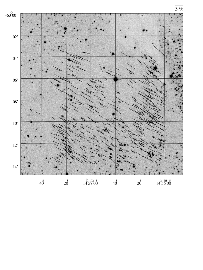
Figure 1: Polarimetry of the Field 17 which contains HH 76-77 and HH 139. Upper panel: The observed polarization vectors overplotted on a DSS2 red image. The coordinates are B1950. Lower panel: The histogram of the corresponding position angles of the polarization, $\theta$. In the upper right corner, it is shown the average and the dispersion of the interstellar magnetic field used in the analysis. A Gaussian curve using these values is also depicted.

Figure 2: Cumulative histogram of the difference between the position angle of the jet and the direction of the ISMF ($\Delta\theta$). $\rm{F_{cum}}$ represents the cumulative fraction of objects with $\Delta\theta$ smaller than a given value. The solid line is the observed distribution and the dashed line represents a uniform distribution for comparison. In the upper left corner, it is shown the probability that the observed $\Delta\theta$ is drawn from a uniform distribution according to the Kuiper test (Kp1).

Figure 3: Cumulative histograms of $\Delta\theta$ for all objects having an estimate for their Class (solid line). The histogram for objects of Classes 0 and I is shown as a dashed line and that for objects of Class II as a dotted line. The dot-dash-dot line corresponds to a uniform distribution. It is also shown the probability that each distribution comes from a uniformly distributed population according to the Kuiper test.

Figure 4: Cumulative histograms of $\Delta\theta$ for all the objects of our sample that have the mass determined (solid line), for the low mass objects (dashed line) and for intermediate and high mass objects (dotted line). It is also shown the resulting probability from a Kuiper test comparing each observed distribution with the uniform one.

Figure 5: Cumulative histogram of the dispersion of the interstellar magnetic field, $\sigma_{B}$, for all fields, for fields having objects classified as Classes 0 or I and for regions with objects of Class II.

Figure 6: Cumulative histogram of the dispersion of the interstellar magnetic field, $\sigma_{B}$, for all fields, for fields having low mass objects (LM) and for regions with objects of intermediate or high mass (IHM).

Figure 7: Average interstellar polarization of a field plotted as a function of the dispersion of the interstellar magnetic field, $\sigma_{B}$.

Figure 8: The average polarization of the ISM as a function of the interstellar extinction. Different symbols are used to represent regions harboring objects with different masses according to the legend.

Table 1: Star forming region or cloud in the direction of each field

Field	Region
1	L1630 - South of NGC2068 - Orion
2	Gum Nebula - Bok globule Sa 111
3	Chamaeleon II dark cloud
4	Lupus 2
5	Norma 1
6	L1641 - Orion
7	L1660 - Vela
8	Near the small nebula Re 6 - Vela Molecular Ridge
9	Southern edge of the small cloud S114 - Gum Nebula
10	R Coronae Australis Molecular Cloud
11	L1641 - Orion
12	Orion B
13	Cometary globule CG30 - Gum Nebula
14	S114 or DC 268.0+1.0 - central part of Vela R2
15	DC 290.4+01.9, near the bright-rimmed HII region BBW 47 - eastern Carina
16	DC 291.4-02 - Globule No. 103 - Sandqvist No. 127 (S127)
17	G317-4 - Western end of the Circinus molecular cloud complex
18	Main Circinus core, western part of the Circinus complex
19	S296
20	DC 278.6-0.9 - Vela
21	S109 - Gum Nebula
22	Puppis/Vela
23	L1634 - Orion
24	GGD 17 - Monoceros R2
25	Small cometary globule Ori I-2 - Orion
26	BHR 71 - a Bok Globule
27	Trifid Nebula
28	Orion 1b association

Table 2: Journal of observations

Field	HHs	AR	Dec	Filter	$n_{im}$	$t_{exp}$	Date Obs.
	in the field	B1950				(s)
1	19, 20, 21, 22,	05 42 30	00 00 00	$R_{C}$	12	200	2005 Feb 15
	23, 24, 25, 26,
	27, 37, 70
2	46, 47	08 24 17	-50 50 34	$R_{C}$	9	600	1998 Dec 18
3	52, 53, 54	12 50 20	-76 42 30	$R_{C}$	12	200	2005 Feb 16
4	55	15 52 50	-37 37 37	$R_{C}$	12	200	2005 Feb 16
5A	56, 57	16 28 45	-44 48 20	$R_{C}$	8	10	2005 Feb 12
5B	56, 57	16 28 45	-44 48 20	$R_{C}$	8	300	2005 Feb 12
6	68, 69	05 39 10	-06 27 00	$R_{C}$	9	200	2005 Feb 17
7	72	07 18 00	-23 59 00	$R_{C}$	16	300	2005 Feb 13
8	73, 74	09 01 15	-44 39 00	$R_{C}$	8	60	2007 May 07
9	75	09 09 35	-45 34 00	$R_{C}$	12	180	2005 Feb 17
10	82, 96, 97,	18 57 42	-37 14 00	$R_{C}$	8	100	2007 May 07
	98, 99, 100,
	101, 104, 729,
	730, 731, 732,
	733,734, 735,
	736, 860
11	59, 60, 83	05 31 00	-06 32 00	$R_{C}$	16	300	2005 Feb 14
12A	90, 91, 92, 93,	05 38 57	-01 08 00	$R_{C}$	8	200	2005 Feb 16
	597, 598
12B	90, 91, 92, 93,	05 39 10	-00 57 30	$R_{C}$	8	250	2005 Feb 16
	597, 598
13A	120	08 07 47	-35 59 48	$R_{C}$	8	20	2005 Feb 14
13B	120	08 07 47	-35 59 48	$R_{C}$	8	300	2005 Feb 14
14	133	09 08 35	-45 14 00	$R_{C}$	12	250	2005 Feb 17
15	135, 136	11 10 00	-58 30 00	$R_{C}$	16	300	2005 Feb 12
16	137, 138	11 11 30	-60 37 00	$R_{C}$	16	120	2005 Feb 16
17	76, 77, 139	14 56 51	-63 07 28	$R_{C}$	16	300	2005 Feb 13
18A	140, 141, 142,	14 59 00	-63 12 00	$R_{C}$	4	10	2005 Feb 14
	143
18B	140, 141, 142,	14 59 00	-63 12 00	$R_{C}$	6	300	2005 Feb 14
	143
19	160	07 01 37	-11 26 00	$R_{C}$	8	40	2005 Feb 17
20	171	09 46 45	-54 42 30	$R_{C}$	16	60	2005 Feb 15
21	188, 246	08 19 05	-49 29 30	$R_{C}$	16	300	2005 Feb 13
22	217	08 15 39	-35 43 43	$R_{C}$	16	150	2005 Feb 17
23	240, 241	05 17 27	-06 00 06	$R_{C}$	8	600	2005 Feb 11
24A	271, 272,	06 10 25	-06 11 00	$R_{C}$	8	250	2005 Feb 16
	273
24B	271, 272,	06 10 07	-06 23 00	$R_{C}$	8	100	2005 Feb 16
	273
25	289	05 35 40	-01 46 00	$R_{C}$	8	300	2005 Feb 15
26	320, 321	11 58 40	-64 59 00	$R_{C}$	16	120	2005 Feb 16
27	399	17 59 20	-23 10 00	$R_{C}$	8	100	2007 May 07
28	444, 445,	05 37 15	-02 31 00	$R_{C}$	16	250	2005 Feb 15
	446, 447

Note. — $n_{im}$ is the number of images and $t_{exp}$ is the exposure time of each image.

Table 3: Interstellar polarization and extinction in the observed fields

Field	$N_{f}$	$\theta_{P}$	$\theta_{B}$	$\sigma_{B}$	$P_{ISM}$	A(V)
		(deg)	(deg)	(deg)	(%)	(mag)
1	53	173	173	8.0	2.21	2.0
2	166	136	136	7.0	1.74	3.3
3	95	108	108	14.3	1.57	3.8
4	69	12	12	17.1	0.73	1.7
5	336	51	51	11.5	1.87	5.9
6	27	131	131	7.6	1.46	3.7
7	175	116	116	21.0	0.42	6.1
8	19	135	135	5.3	0.24	13.3
9	176	177	177	12.4	1.04	7.3
10	15	20	20	23.1	0.08	2.6
11	18	53	53	9.6	0.32	0.7
12A	14	50	50	11.3	0.55	1.0
12B	44	160	160	7.7	0.47	0.9
13	234	47/101	101	7.5	0.39	4.9
14	289	24	24	8.3	2.24	6.6
15	502	60/103	41	21.7	0.52	17.9
16	509	86/170	171	11.4	0.58	13.5
17	559	59	59	7.0	2.56	4.7
18	139	68	68	9.3	2.08	4.6
19	72	57/150	150	16.5	0.29	7.2
20	105	142	142	7.1	0.99	7.6
21	129	109	109	7.8	2.92	4.7
22	279	108	108	12.4	1.03	9.2
23	17	39	39	18.2	0.31	1.2
24A	22	163	163	25.8	0.41	1.4
24B	38	151	151	12.4	0.15	1.4
24AB	60	152	152	16.9	0.19	1.4
25	44	161	161	29.9	0.32	0.6
26	497	102	102	9.3	1.31	5.4
27	179	175	175	14.7	0.43	61.7
28	51	83/147	151	7.9	0.90	0.8

Table 4: Polarimetric catalog

Field	ID	RA	Dec	P	PA
		(1950.0)	(1950.0)	(%)	(deg)
Field 01
1	1	5 42 14.94	+00 02 07.90	1.83$\pm$0.12	165.0
1	2	5 42 15.04	+00 01 26.40	2.21$\pm$0.10	169.5
1	3	5 42 15.24	+00 02 56.09	1.96$\pm$0.04	166.8
1	4	5 42 15.82	-00 06 09.76	3.76$\pm$0.79	173.8
1	5	5 42 17.40	-00 01 06.54	2.82$\pm$0.51	162.9

Note. — Table 4 is published in its entirety in the electronic edition of the Astrophysical Journal. A portion is shown here for guidance regarding its form and content.

Table 5: Jet Information

Jet	Distance	Reference	Extension	Reference	PA	Reference
	(pc)		(pc)		(°)
24J,19/24K,27	450	21	0.95/0.68	21	132	Visual (21,52)
24C,20/24E,24M	450	21	1.09/0.11	21	153	40
24G	500	40	0.24	40	38	40
22	450	21	0.40	21	76	Visual (21)
23	450	21	0.37	21	8	Knots (21)
24A/25B	400	24	0.13	This work (24,35)	40	24,35
25A/25D	400	24	0.07	This work (24,35)	164	24,35
26A/26B	400	24	0.07	This work (24,35)	50	24,35
46/47	460,450	18,61	1.3	30	56	64,71
52,53,54	130	9	0.39	This work (54)	60	Visual (54)
55	150-250	27	0.04	27	160	27
56	700,900:	55,9	0.38	65	36	Knots (65)
57	700,900:	55,9	0.02	This work (65)	19	Knots (65)
59	460	15	0.05	63	0	15
60	460	15	0.47	15	124	15
68	460	68	0.15	This work (4)	156	15
69	460	15	0.26	This work (63)	158:	15
72	1500	24	0.44	This work (63)	79	24
73	450	52	0.15	52	146	Visual (63)
74	450	15	0.13	This work (37,75)	93	Knots (37,75)
75	450,870	15,63	1	This work (63)	152	15
76	700,500-1000	6,63	0.04	63	148	15
77	700,750	6,15	$\cdots$	$\cdots$	119	15
82	129,170	63,74	0.07	This work (63)	100	63
83/83	470,480	5,39	0.43	40	125	40
90-93,597,598	415	7	2.05	7	131	7
96-98,100,101	129,170	63,74	$>$0.09	This work (74)	32	Visual (74)
99,104C-D,730,860	129,170	63,74	0.26	74	58	Visual (74)
120	450	13	0.01	70	110	Visual (28)
133	870	46	0.32	This work (46)	105	46
135/136	2700-2900	50	0.55	50	39	67
137	2200	47	0.84	This work (47)	103	47
138	2200	47	0.23	This work (47)	106	Knots (47)
139	700,1500	6,29	0.005 or 0.01	This work (6,29)	100	6
140	2900,700	56,6	1.8 or 0.43	This work (56,6)	135	Visual (56)
141	2900,700	56,6	0.42 or 0.1	This work (56,6)	95	Visual (56)
142,143	2900,700	56,6	1.31 or 0.32	This work (56,6)	135	56
160	1150	59	1.8	53	60	73
171	$\cdots$	$\cdots$	$\cdots$	$\cdots$	60	48
188	450	25	1.2	25	149	25
217	4300	41	0.40	41	60	Visual (36,41,58)
240/241	460,500	45,18	0.40	18	103	Visual (18)
246	450	26	0.02	26	115	26
271-272	830	14	0.72	14	165	Visual (8,14)
273	830	14	$\cdots$	$\cdots$	$\cdots$	$\cdots$
289	470	38	0.62	38	65	Visual (38)
320	200	11	0.06	This work (24)	144	24
321	200	11	0.08	This work (24)	0	24
399	1680,1670-2670	66,76	0.14	76	20	Visual (76)
444	360-470	60	0.35	60	66	Knots (38,60)
445	360-470	60	0.28	60	103	Visual (60)
445X	360-470	60	0.03	This work (60)	78	Visual (60)
446	360-470	60	0.03	60	168	Visual (60)
447	360-470	60	0.02	60	32	Visual (60)
729	129,170	63,74	0.07	This work (74)	115	74
731	129,170	63,74	$\cdots$	$\cdots$	$\cdots$	$\cdots$
732	129,170	63,74	$>$0.03	This work (74)	157	Visual (74)
733	129,170	63,74	0.16	This work (74)	35	Visual (74)
734	129,170	63,74	$\cdots$	$\cdots$	129	Visual (74)
735,736	129,170	63,74	$\cdots$	$\cdots$	$\cdots$	$\cdots$

Note. — The numbers in the first column correspond to the HHs that define a jet. HHs separated by “/” correspond to jet and counter-jet. Colon is used to indicate uncertainty.

References. — We use the same numeration for references in this table and in Table Correlating the interstellar magnetic field with protostellar jets and its sources. (1) Ábrahám et al. (2004a); (2) Ábrahám et al. (2004b); (3) Andrews et al. (2004); (4) Avila et al. (2001); (5) Bally et al. (1994); (6) Bally et al. (1999); (7) Bally et al. (2002); (8) Beltrán et al. (2001); (9) Berrilli et al. (1989); (10) Bohigas et al. (1993); (11) Bourke (2001); (12) Brittain et al. (2007); (13) Caratti o Garatti et al. (2006); (14) Carballo & Eiroa (1992); (15) Cohen (1990); (16) Connelley et al. (2007); (17) Corporon & Reipurth (1997); (18) Davis et al. (1997); (19) Dent et al. (1998); (20) Dobashi et al. (1998); (21) Eisloffel & Mundt (1997); (22) Felli et al. (1998); (23) Forbrich & Preibisch (2007); (24) Giannini et al. (2004); (25) Girart & Viti (2007); (26) Graham (1986); (27) Graham & Chen (1994); (28) Gredel (1994); (29) Gyulbudaghian & May (2005); (30) Hartigan et al. (2005); (31) Heyer & Graham (1990); (32) Huélamo et al. (2007); (33) Jijina et al. (1999); (34) Lefloch et al. (2002); (35) Lis et al. (1999); (36) Liseau et al. (1992); (37) Lorenzetti et al. (2002); (38) Mader et al. (1999); (39) Miesch & Bally (1994); (40) Mundt et al. (1991); (41) Neckel & Staude (1995); (42) Nielbock & Chini (2005); (43) Nisini et al. (1996); (44) Noriega-Crespo et al. (2004); (45) O’Connell et al. (2004); (46) Ogura (1990); (47) Ogura (1993); (48) Ogura & Noumaru (1994); (49) Ogura & Walsh (1991); (50) Ogura & Walsh (1992); (51) Persi et al. (1994); (52) Podio et al. (2006); (53) Poetzel et al. (1989); (54) Porras et al. (2007); (55) Prusti et al. (1993); (56) Ray & Eisloeffel (1994); (57) Reipurth (1989); (58) Reipurth (1994); (59) Reipurth (2000); (60) Reipurth et al. (1998); (61) Reipurth & Cernicharo (1995); (62) Reipurth et al. (1993); (63) Reipurth & Graham (1988); (64) Reipurth & Heathcote (1991); (65) Reipurth et al. (1997); (66) Rho et al. (2006); (67) Rodrigues et al. (2007); (68) Rodriguez & Reipurth (1994); (69) Rolph et al. (1990); (70) Schwartz & Greene (2003); (71) Stanke et al. (1999); (72) Thi et al. (2006); (73) Velázquez & Rodríguez (2001); (74) Wang et al. (2004); (75)Wu et al. (2002); (76) Yusef-Zadeh et al. (2005)

Table 6: Information about the young stellar objects associated with the jets of our sample

Jet	Name	Reference	$L_{bol}$	Reference	Mass	Reference	Class	Reference
			($L\odot$)
24J,19/24K,27	SSV 63W	21	$<$20	35,62	$\cdots$	$\cdots$	I	35
24C,20/24E,24M	SSV 63E	21	$<$20	35,62	$\cdots$	$\cdots$	I	32
24G	SSV 63NE	40	$<$ 20	35,62	low	32	$\cdots$	$\cdots$
22	$\cdots$	$\cdots$	$\cdots$	$\cdots$	$\cdots$	$\cdots$	$\cdots$	$\cdots$
23	IRAS 05436-0007, V1647 Ori	21,12	6	2	low	2	I/II	12,2
24A/25B	HH24MMS	24	5	24	$\cdots$	$\cdots$	0	24
25A/25D	HH25MMS,VLA2	24,35	6,24	24,35	$\cdots$	$\cdots$	0	24
26A/26B	HH26IR	24	29	24	$\cdots$	$\cdots$	I	24
46/47	IRAS 08242-5050	62	24,12,19	9,44,62	low	19	I	44
52,53,54	IRAS 12496-7650	43	$\cdots$	$\cdots$	int	43	$\cdots$	$\cdots$
55	IRAS 15533-3742,HH55star	27,31	$<$0.3	31,27,9	low	27	II/III	27
56	Re 13	55	50	55	$\cdots$	$\cdots$	I	55
57	V346 Nor	42	135	55	low	1	I	42
59	$\cdots$	$\cdots$	$\cdots$	$\cdots$	$\cdots$	$\cdots$	$\cdots$	$\cdots$
60	IRAS 05299-0627c	19	1	15	$\cdots$	$\cdots$	$\cdots$	$\cdots$
68	IRAS 05391-0627c:,HH68b:	15,4	10	15	$\cdots$	$\cdots$	$\cdots$	$\cdots$
69	IRAS 05393-0632:	15	25	15	$\cdots$	$\cdots$	$\cdots$	$\cdots$
72	IRAS 07180-2356	24	170,316	13,15	$\cdots$	$\cdots$	I	13
73	unknown	52	$\cdots$	$\cdots$	$\cdots$	$\cdots$	$\cdots$	$\cdots$
74	IRAS 09003-4438C	15	6	15	$\cdots$	$\cdots$	$\cdots$	$\cdots$
75	IRAS 09094-4522:	15	130	15	int	72	I	72
76	IRAS 14563-6250	62	21	15	$\cdots$	$\cdots$	I	6
77	IRAS 14564-6254	15	47	63	$\cdots$	$\cdots$	$\cdots$	$\cdots$
82	S CrA	63	2	62	low	63	II	63
83	IRAS 05311-0631	52	9	33	low	5	II	16
90-93,597,598	IRAS 05399-0121	7	10	7	low	7	I	16
96-98,100,101	IRS1/HH100-IRS	74	3	23	$\cdots$	$\cdots$	I	74
99,104C-D,730,860	IRS 6	74	1	23	$\cdots$	$\cdots$	II	23
120	IRAS 08076-3556	13	13-19	13	low	51	I	13
133	$\cdots$	$\cdots$	$\cdots$	$\cdots$	low:	46	$\cdots$	$\cdots$
135/136	IRAS 11101-5829	75	14000	50	high	50	0/I	67
137,138	unknown	47	$\cdots$	$\cdots$	$\cdots$	$\cdots$	$\cdots$	$\cdots$
139	IRAS 14568-6304	6	133	20	low	6	I,II	6,29
140	IRAS 14592-6311	75	2400	56	int	56	$\cdots$	$\cdots$
141	$\cdots$	$\cdots$	$\cdots$	$\cdots$	$\cdots$	$\cdots$	$\cdots$	$\cdots$
142,143:	$\cdots$	$\cdots$	$\cdots$	$\cdots$	$\cdots$	$\cdots$	$\cdots$	$\cdots$
160	Z CMa,IRAS 07013-1128	19	3500,3000	53,73	int	53	I/II	53
171	IRAS 09469-5443:	48	$\cdots$	$\cdots$	$\cdots$	$\cdots$	$\cdots$	$\cdots$
188	IRAS 08194-4925	25	30	25	low	25	0/I	25
217	IRAS 08159-3543	58	2400	22	int	22	I	22
240/241	IRAS 05173-0555	18	17-27	13	low	10	I	13
246	HD180617	26	$\cdots$	$\cdots$	low	26	$\cdots$	$\cdots$
271,272	Bretz 4,IRAS 06103-0612	14,8	4	8	low	14	II	8,14
273	$\cdots$	$\cdots$	$\cdots$	$\cdots$	$\cdots$	$\cdots$	$\cdots$	$\cdots$
289	IRAS 05355-0146	38	13	38	$\cdots$	$\cdots$	$\cdots$	$\cdots$
320	BHR71(IRS2)	13	1-3	13	low	17	I	13
321	BHR71-MM(IRS1)	13	8-10	13	low	17	0	13
399	TC2	66	600	66	high	34	0/I	66
444	V510 Ori	38	variable	60	low	3	II	38
445	A0976-357	60	$\cdots$	$\cdots$	low	60	II	60
445X	A0976-357	60	$\cdots$	$\cdots$	low	60	II	60
446	$\cdots$	$\cdots$	$\cdots$	$\cdots$	low	3	II	60
447	Haro5-39	60	$\cdots$	$\cdots$	low	60	II	60
729	S CrA	74	2	63	low	63	II	63
731	IRS1, 2 or 5	74	$\cdots$	$\cdots$	$\cdots$	$\cdots$	I	74
732	$\cdots$	$\cdots$	$\cdots$	$\cdots$	$\cdots$	$\cdots$	$\cdots$	$\cdots$
733	T CrA	74	3	23	low	23	II	23
734	K-ex or WMB 55	74	$\cdots$	$\cdots$	$\cdots$	$\cdots$	$\cdots$	$\cdots$
735,736:	IRS7 or MMS19:	74	$\cdots$	$\cdots$	$\cdots$	$\cdots$	$\cdots$	$\cdots$

Note. — The numbers in the first column correspond to the HHs that define a jet. HHs separated by ”/” correspond to jet and counter-jet. The luminosities were rounded to integer values. Colon indicates uncertainty.

References. — We use the same numeration for references in this table and in Table Correlating the interstellar magnetic field with protostellar jets and its sources. (1) Ábrahám et al. (2004b); (2) Ábrahám et al. (2004a); (3) Andrews et al. (2004); (4) Avila et al. (2001); (5) Bally et al. (1994); (6) Bally et al. (1999); (7) Bally et al. (2002); (8) Beltrán et al. (2001); (9) Berrilli et al. (1989); (10) Bohigas et al. (1993); (11) Bourke (2001); (12) Brittain et al. (2007); (13) Caratti o Garatti et al. (2006); (14) Carballo & Eiroa (1992); (15) Cohen (1990); (16) Connelley et al. (2007); (17) Corporon & Reipurth (1997); (18) Davis et al. (1997); (19) Dent et al. (1998); (20) Dobashi et al. (1998); (21) Eisloffel & Mundt (1997); (22) Felli et al. (1998); (23) Forbrich & Preibisch (2007); (24) Giannini et al. (2004); (25) Girart & Viti (2007); (26) Graham (1986); (27) Graham & Chen (1994); (28) Gredel (1994); (29) Gyulbudaghian & May (2005); (30) Hartigan et al. (2005); (31) Heyer & Graham (1990); (32) Huélamo et al. (2007); (33) Jijina et al. (1999); (34) Lefloch et al. (2002); (35) Lis et al. (1999); (36) Liseau et al. (1992); (37) Lorenzetti et al. (2002); (38) Mader et al. (1999); (39) Miesch & Bally (1994); (40) Mundt et al. (1991); (41) Neckel & Staude (1995); (42) Nielbock & Chini (2005); (43) Nisini et al. (1996); (44) Noriega-Crespo et al. (2004); (45) O’Connell et al. (2004); (46) Ogura (1990); (47) Ogura (1993); (48) Ogura & Noumaru (1994); (49) Ogura & Walsh (1991); (50) Ogura & Walsh (1992); (51) Persi et al. (1994); (52) Podio et al. (2006); (53) Poetzel et al. (1989); (54) Porras et al. (2007); (55) Prusti et al. (1993); (56) Ray & Eisloeffel (1994); (57) Reipurth (1989); (58) Reipurth (1994); (59) Reipurth (2000); (60) Reipurth et al. (1998); (61) Reipurth & Cernicharo (1995); (62) Reipurth et al. (1993); (63) Reipurth & Graham (1988); (64) Reipurth & Heathcote (1991); (65) Reipurth et al. (1997); (66) Rho et al. (2006); (67) Rodrigues et al. (2007); (68) Rodriguez & Reipurth (1994); (69) Rolph et al. (1990); (70) Schwartz & Greene (2003); (71) Stanke et al. (1999); (72) Thi et al. (2006); (73) Velázquez & Rodríguez (2001); (74) Wang et al. (2004); (75)Wu et al. (2002); (76) Yusef-Zadeh et al. (2005)

Table 7: Proposed new coordinates for HH 140-143

HH	Knot	AR (1950.0)	DEC (1950.0)
140	C	14 59 12	-63 10 44
	D	14 59 26	-63 12 43
141	A	14 59 15	-63 12 33
	D	14 59 10	-63 12 28
142		14 59 25	-63 10 38
143		14 59 35	-63 11 52

From this page on, complementary graphs of Figure 1. They will appear as online-only material.

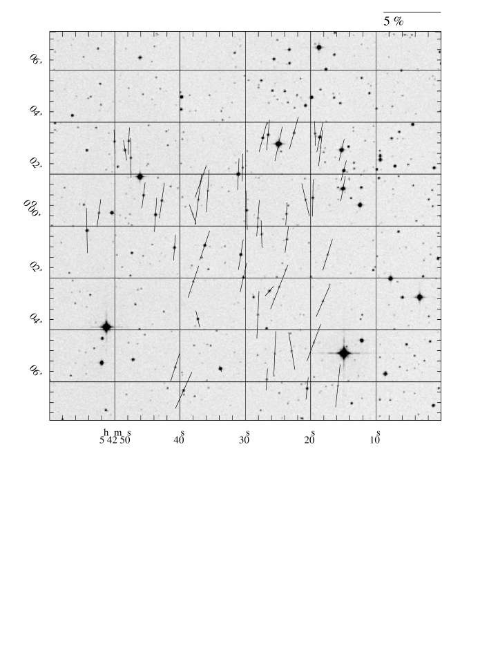
Polarimetry of Field 01. Upper panel: The observed polarization vectors overplotted on a DSS2 red image. The coordinates are B1950. Lower panel: The histogram of the corresponding position angles of the polarization, $\theta$. In the upper right corner, it is shown the average and the dispersion of the interstellar magnetic field used in the analysis. A Gaussian curve using these values is also depicted.

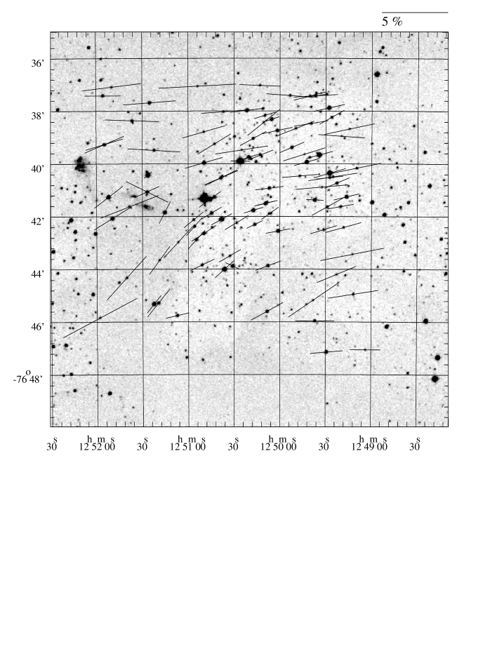
The same of Figure 1 for Field 03.

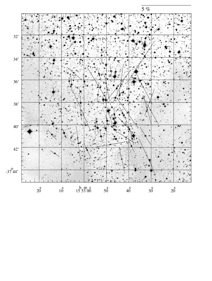
The same of Figure 1 for Field 04.

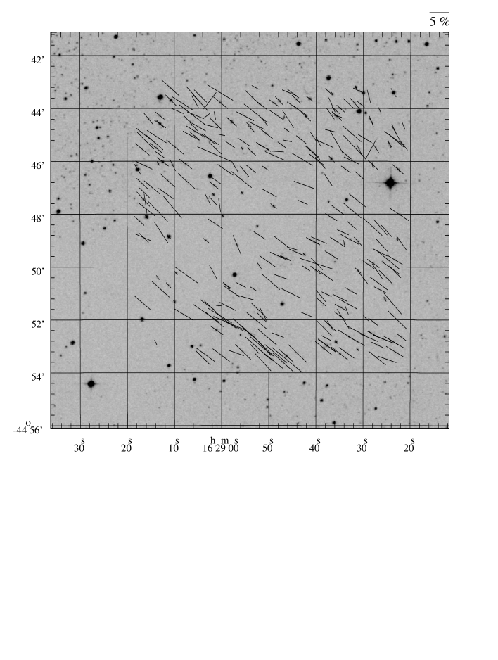
The same of Figure 1 for Field 05.

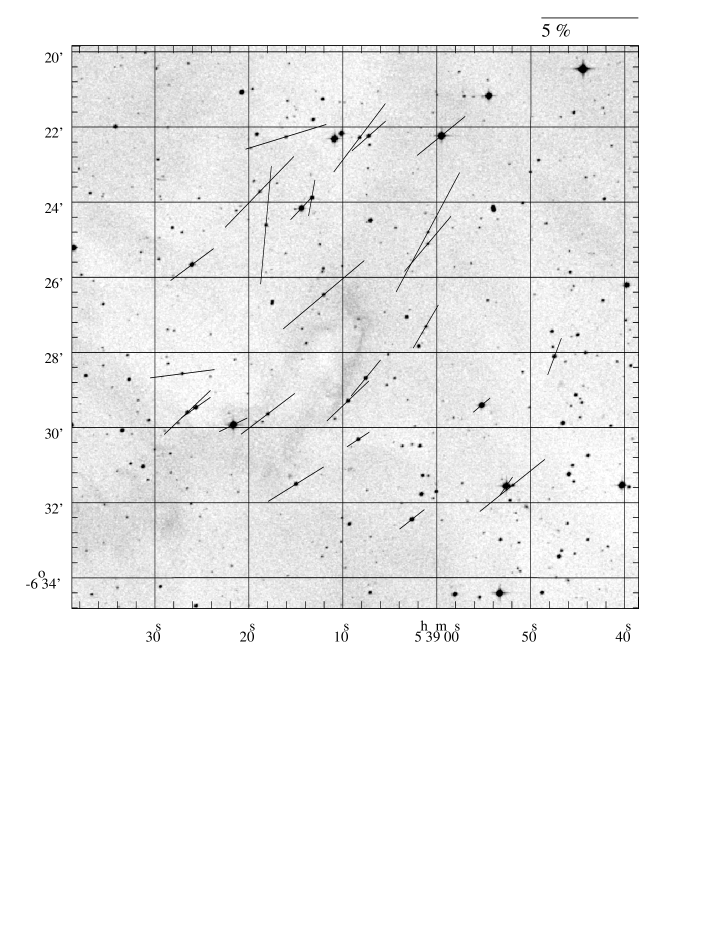
The same of Figure 1 for Field 06.

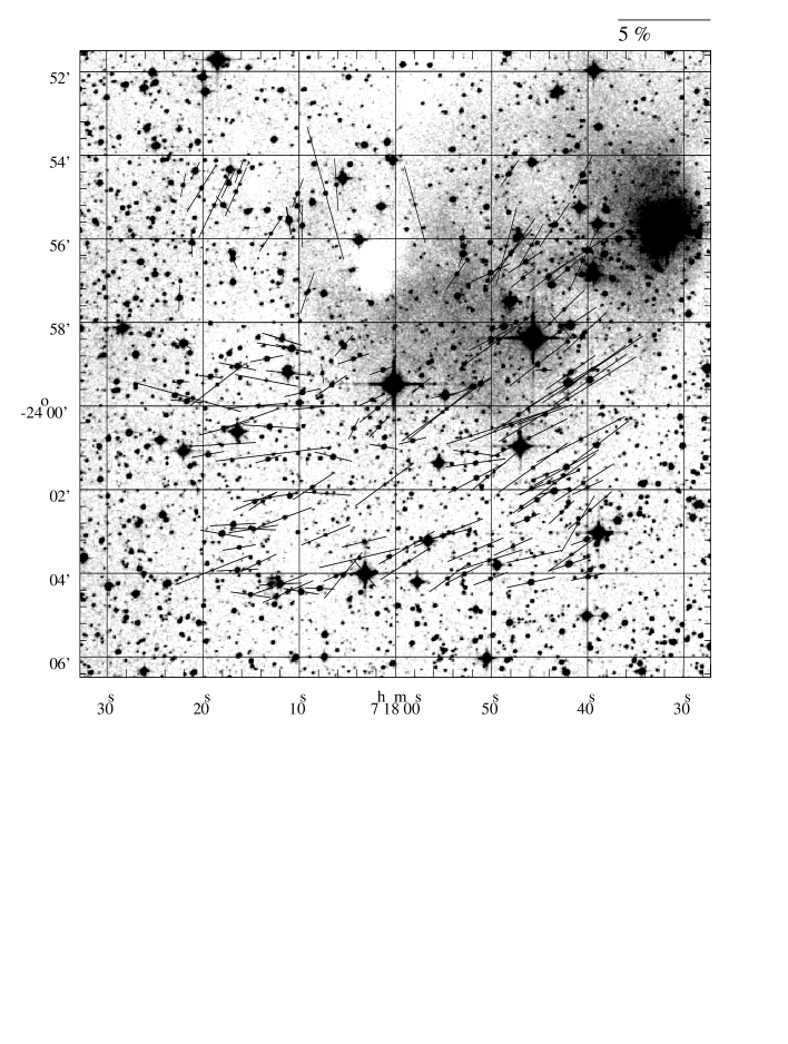
The same of Figure 1 for Field 07.

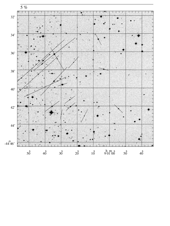
The same of Figure 1 for Field 08.

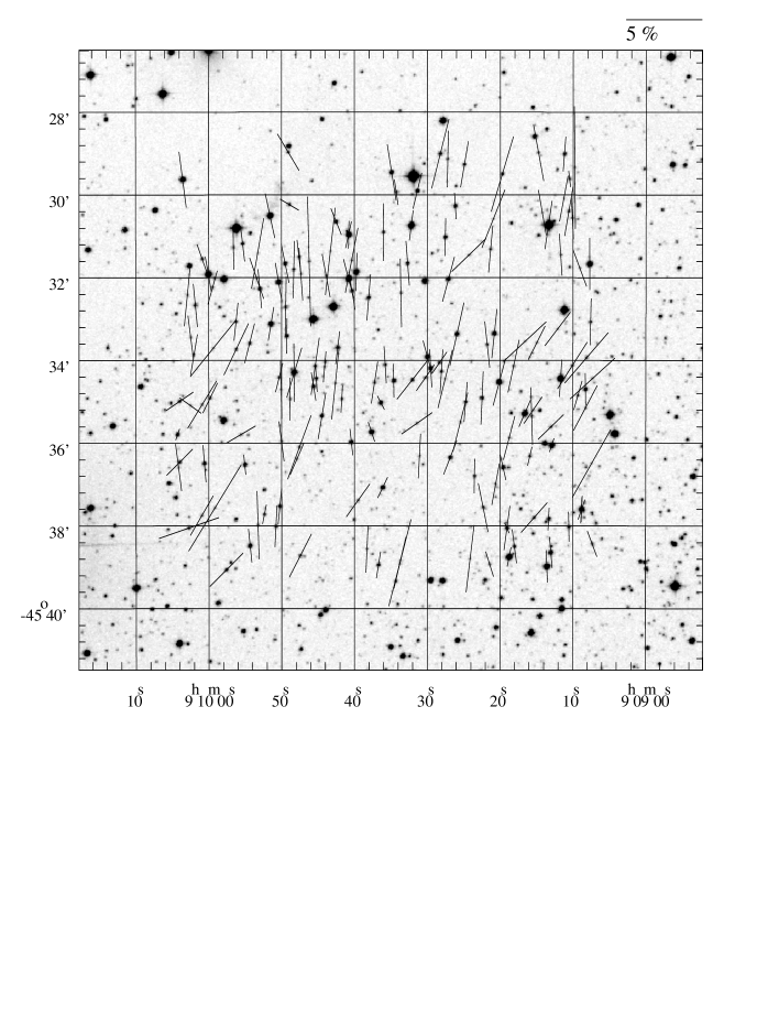
The same of Figure 1 for Field 09.

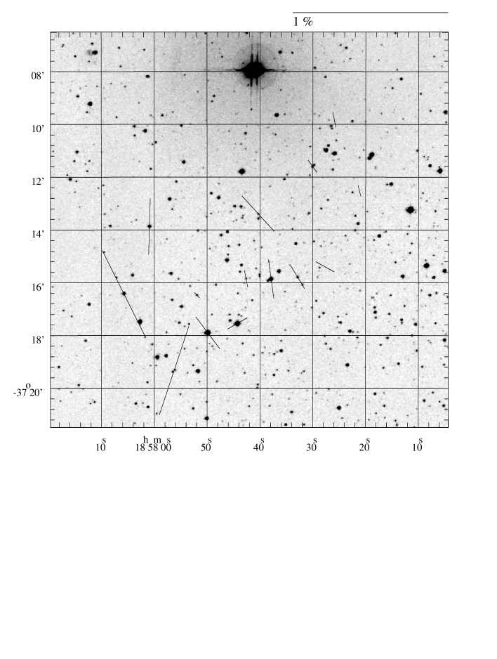
The same of Figure 1 for Field 10.

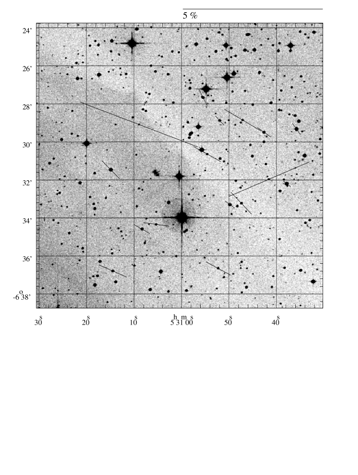
The same of Figure 1 for Field 11.

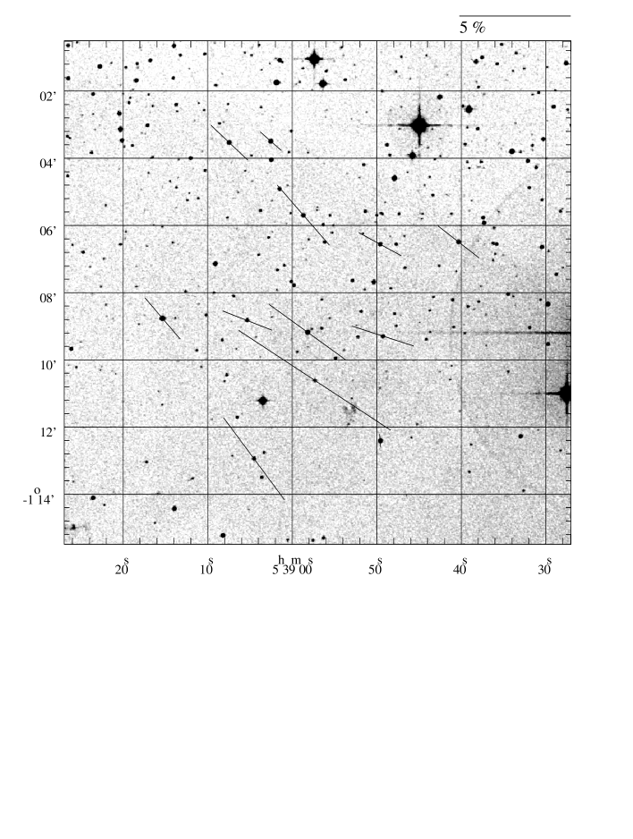
The same of Figure 1 for Field 12A.

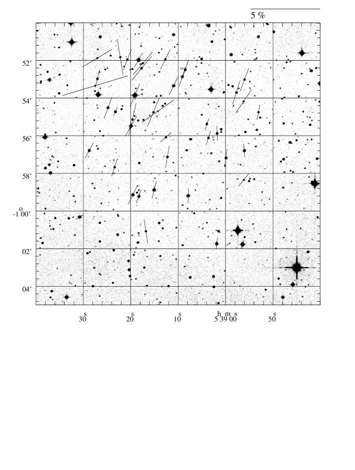
The same of Figure 1 for Field 12B.

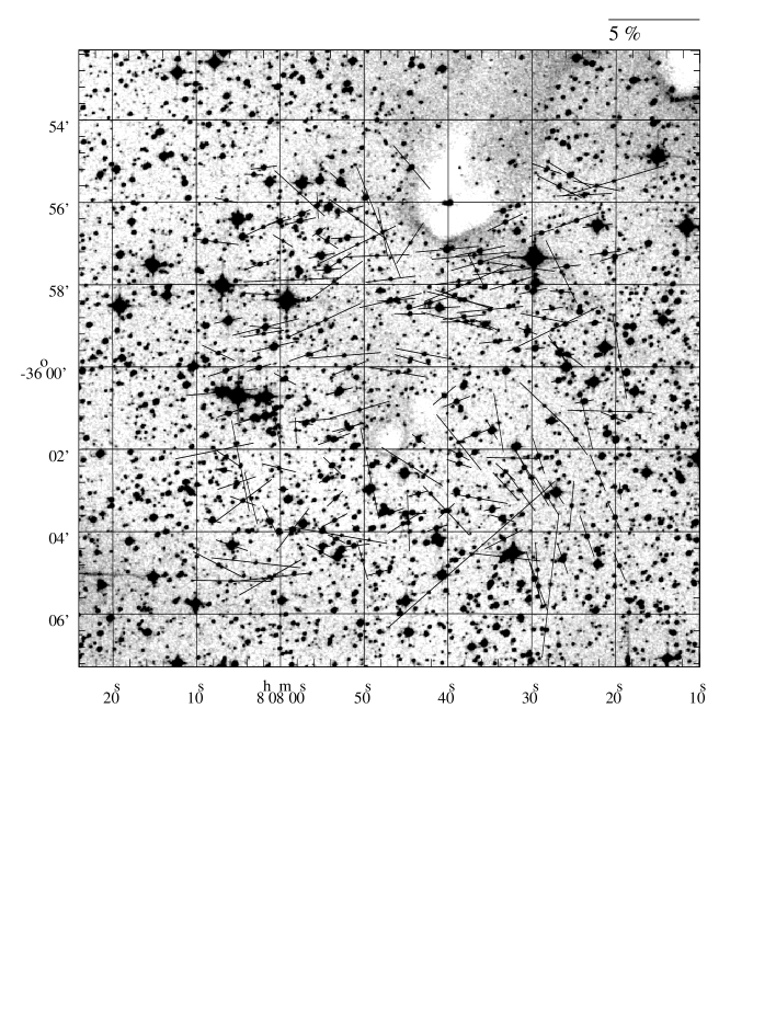
Figure 9: Polarimetry of Field 13. Upper panel: The observed polarization vectors overplotted on a DSS2 red image. The coordinates are B1950. Lower panel: The histogram of the corresponding position angles of the polarization, $\theta$. In the upper right corner, it is shown the average and the unbiased dispersion of the interstellar magnetic field used in the analysis. The solid line is the respective Gaussian curve. The dashed lines represent the two Gaussian fits used to separated the polarimetric components and the dot-dash line is the sum of these two components.

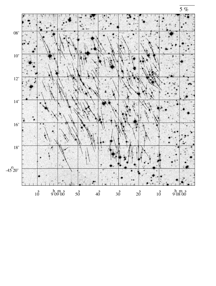
The same of Figure 1 for Field 14.

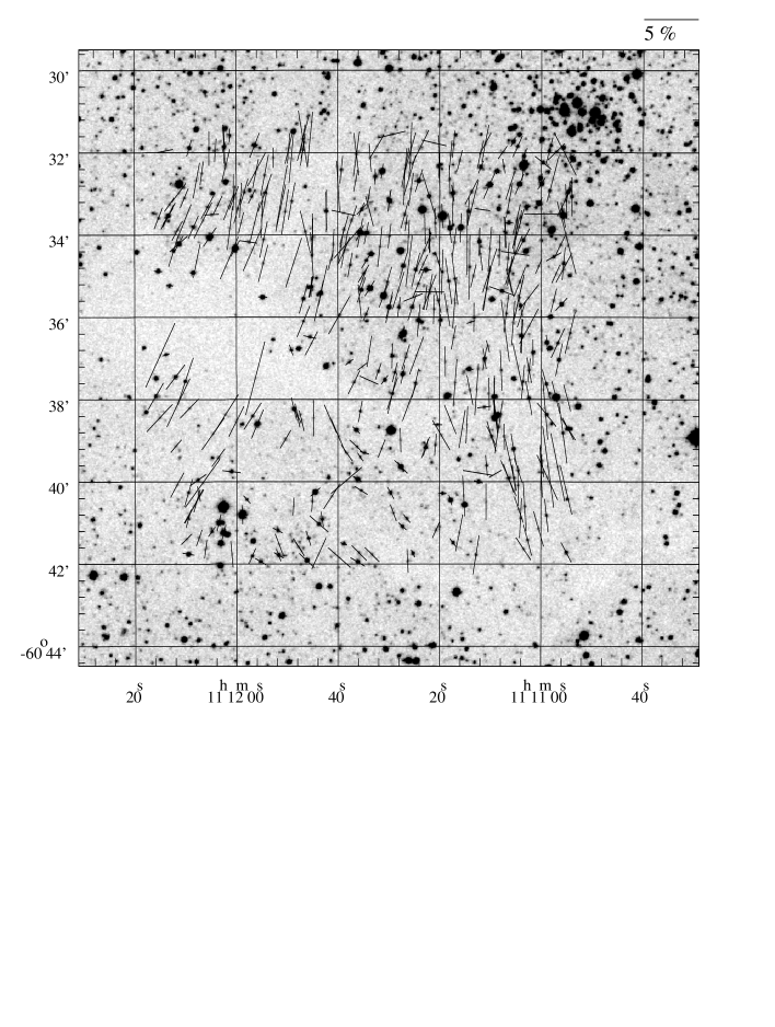
The same of Figure 1 for Field 16.

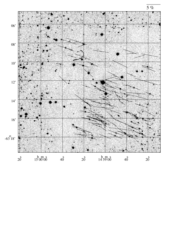
The same of Figure 1 for Field 18.

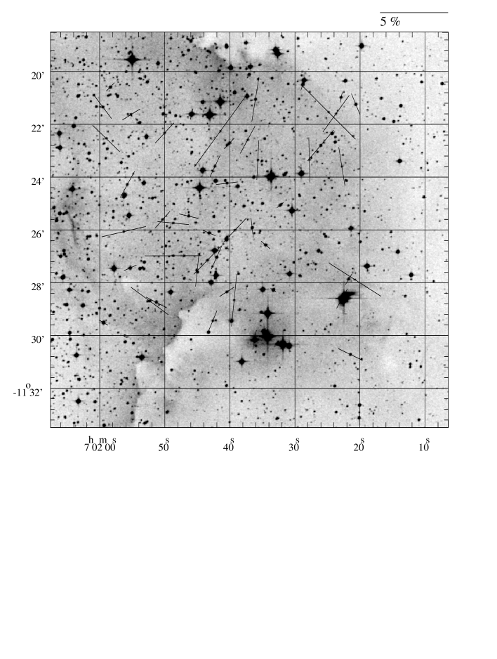
The same of Figure 1 for Field 19.

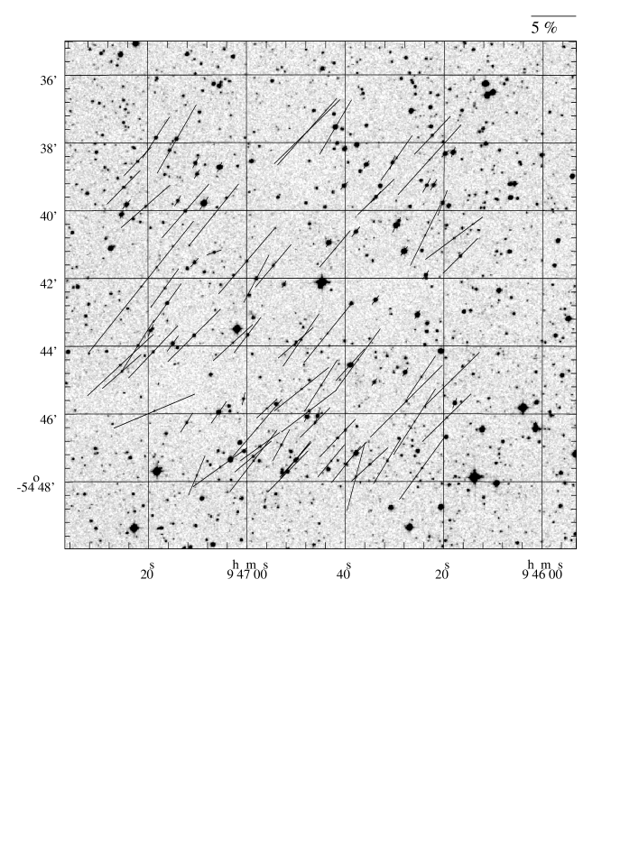
The same of Figure 1 for Field 20.

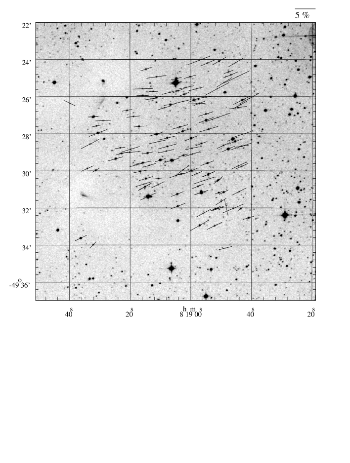
The same of Figure 1 for Field 21.

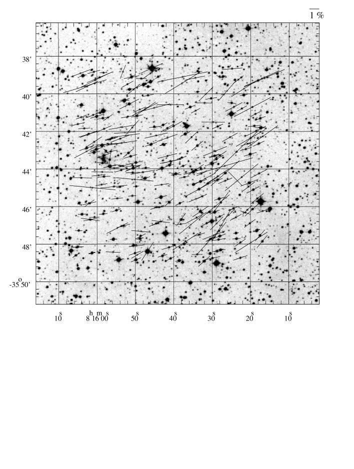
The same of Figure 1 for Field 22.

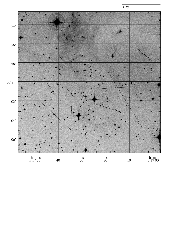
The same of Figure 1 for Field 23.

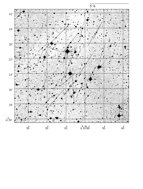
Figure 10: Polarimetry of Fields 24A e 24B. Upper left panel: The observed polarization vectors of Field 24A overplotted on a DSS2 red image. The coordinates are B1950. Upper right panel: The same for Field 24B. Lower panel: The histogram of the position angles of the polarization, $\theta$, of Fields 24A e 24B. In the upper right corner, it is shown the average and the dispersion of the interstellar magnetic field used in the analysis. A Gaussian curve using these values is also depicted.

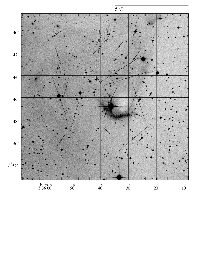
The same of Figure 1 for Field 25.

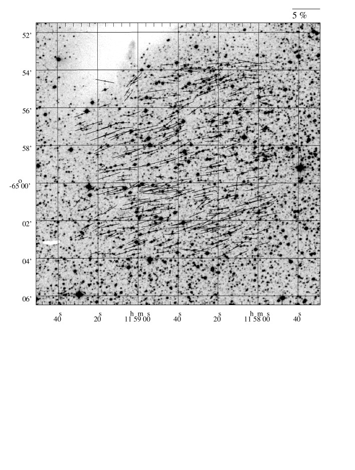
The same of Figure 1 for Field 26.

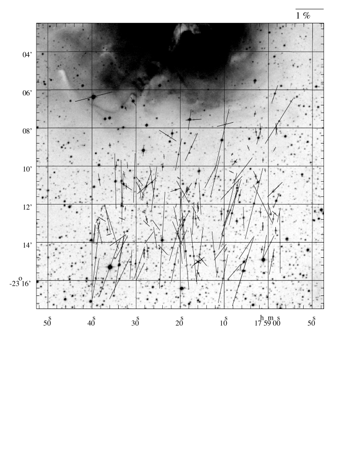
The same of Figure 1 for Field 27.

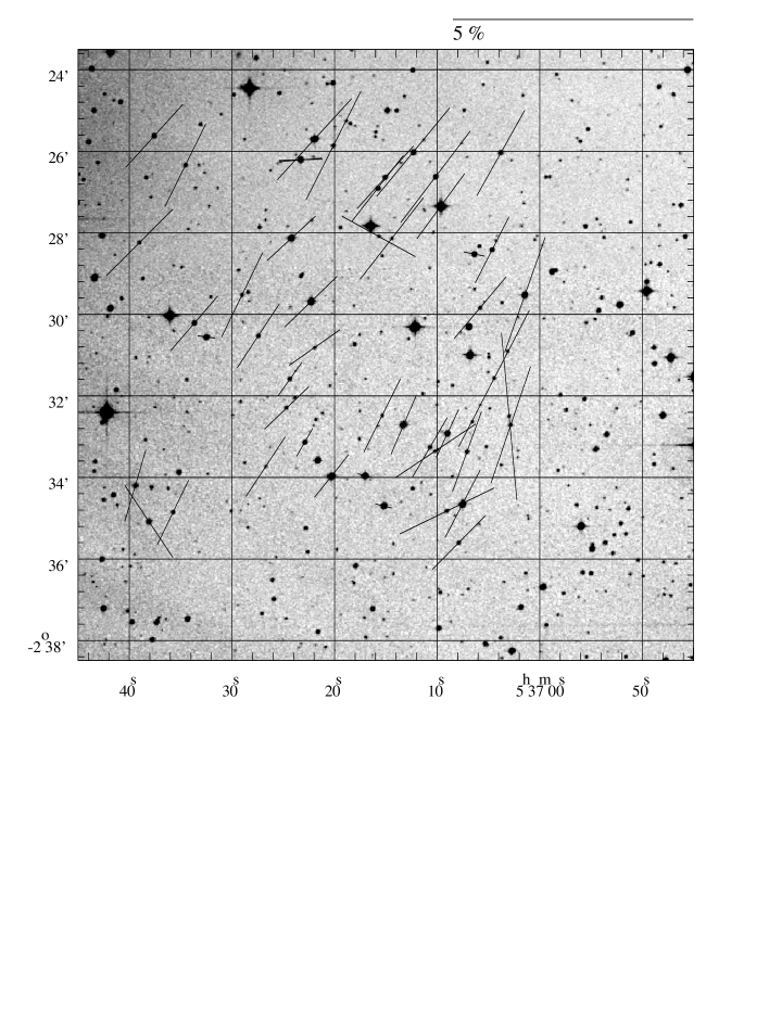
The same of Figure 1 for Field 28.

References

- Ábrahám et al. (2004a) Ábrahám, P., Kóspál, Á., Csizmadia, S., Kun, M., Moór, A. & Prusti, T. 2004, A&A, 428, 89
- Ábrahám et al. (2004b) Ábrahám, P., Kóspál, Á., Csizmadia, S., et al. 2004, A&A, 419, L39
- Alves et al. (2008) Alves, F. O., Franco, G. A. P., & Girart, J. M. 2008, A&A, 486, L13
- Anathpindika & Whitworth (2008) Anathpindika, S., & Whitworth, A. P. 2008, A&A, 487, 605
- Andrews et al. (2004) Andrews, S. M., Reipurth, B., Bally, J. & Heathcote, S. R. 2004, ApJ, 606, 353
- Avila et al. (2001) Avila, R., Rodríguez, L. F. & Curiel, S. 2001, Rev. Mexicana Astron. Astrofis., 37, 201
- Bally et al. (1994) Bally, J., Castets, A. & Duvert, G. 1994, ApJ, 423, 310
- Bally et al. (2002) Bally, J., Reipurth, B. & Aspin, C. 2002, ApJL, 574, L79
- Bally et al. (1999) Bally, J., Reipurth, B., Lada, C. J. & Billawala, Y. 1999, AJ, 117, 410
- Bastien et al. (1988) Bastien, P., Drissen, L., Menard, F., et al. 1988, AJ, 95, 900
- Beltrán et al. (2001) Beltrán, M. T., Estalella, R., Anglada, G., Rodríguez, L. F. & Torrelles, J. M. 2001, AJ, 121, 1556
- Benson & Myers (1989) Benson, P. J., & Myers, P. C. 1989, ApJS, 71, 89
- Berrilli et al. (1989) Berrilli, F., Ceccarelli, C., Liseau, R., et al. 1989, MNRAS, 237, 1
- Bohigas et al. (1993) Bohigas, J., Persi, P., Tapia, M. 1993, A&A, 267, 168
- Bourke (2001) Bourke, T. L. 2001, ApJL, 554, L91
- Brittain et al. (2007) Brittain, S., Rettig, T. W., Simon, T., et al. 2007, ApJL, 670, L29
- Brunt et al. (2009) Brunt, C. M., Heyer, M. H., & Mac Low, M.-M. 2009, A&A, 504, 883
- Caratti o Garatti et al. (2006) Caratti o Garatti, A. and Giannini, T. and Nisini, B. & Lorenzetti, D. 2006, A&A, 449, 1077
- Carballo & Eiroa (1992) Carballo, R. & Eiroa, C. 1992, A&A, 262, 295
- Carroll et al. (2010) Carroll, J. J., Frank, A., & Blackman, E. G 2010, ApJ, 722, 145
- Carroll et al. (2009) Carroll, J. J., Frank, A., Blackman, E. G., Cunningham, A. J., & Quillen, A. C. 2009, ApJ, 695, 1376
- Chandrasekhar & Fermi (1953) Chandrasekhar, S. & Fermi, E. 1953, ApJ, 118, 113
- Cohen (1990) Cohen, M. 1990, ApJ, 354, 701
- Cohen et al. (1984) Cohen, R. J., Rowland, P. R., & Blair, M. M. 1984, MNRAS, 210, 425
- Connelley et al. (2007) Connelley, M. S., Reipurth, B. & Tokunaga, A. T. 2007, AJ, 133, 1528
- Corporon & Reipurth (1997) Corporon, P., & Reipurth, B. 1997, Herbig-Haro Flows and the Birth of Stars, 182, 85P
- Crutcher et al. (2009) Crutcher, R. M., Hakobian, N., & Troland, T. H. 2009, ApJ, 692, 844
- Curran & Chrysostomou (2007) Curran, R. L., & Chrysostomou, A. 2007, MNRAS, 382, 699
- Davis et al. (1997) Davis, C. J., Ray, T. P., Eisloeffel, J. & Corcoran, D. 1997, A&A, 324, 263
- Dent et al. (1998) Dent, W. R. F., Matthews, H. E. & Ward-Thompson, D. 1998, MNRAS, 301, 1049
- Dobashi et al. (1998) Dobashi, K., Sato, F. & Mizuno, A. 1998, PASJ, 50, L15
- Dyck & Lonsdale (1979) Dyck, H. M., & Lonsdale, C. J. 1979, AJ, 84, 1339
- Eisloffel & Mundt (1997) Eisloffel, J. & Mundt, R. 1997, AJ, 114, 280
- Falceta-Gonçalves et al. (2008) Falceta-Gonçalves, D., Lazarian, A., & Kowal, G. 2008, ApJ, 679, 537
- Felli et al. (1998) Felli, M., Taylor, G. B., Neckel, T. & Staude, H. J. 1998, A&A, 329, 243
- Ferreira et al. (2006) Ferreira, J., Dougados, C., & Cabrit, S. 2006, A&A, 453, 785
- Forbrich & Preibisch (2007) Forbrich, J. & Preibisch, T. 2007, A&A, 475, 959
- Franco et al. (2010) Franco, G. A. P., Alves, F. O., & Girart, J. M. 2010, ApJ, 723, 146
- Giannini et al. (2004) Giannini, T., McCoey, C., Caratti o Garatti, A., et al. 2004, A&A, 419, 999
- Girart et al. (2006) Girart, J. M., Rao, R., & Marrone, D. P. 2006, Science, 313, 812
- Girart & Viti (2007) Girart, J. M. & Viti, S. 2007, A&A, 470, 633
- Graham (1986) Graham, J. A. 1986, ApJ, 302, 352
- Graham & Chen (1994) Graham, J. A. & Chen, W. P. 1994, AJ, 108, 2273
- Gredel (1994) Gredel, R. 1994, A&A, 292, 580
- Gyulbudaghian & May (2005) Gyulbudaghian, A. L. & May, J. 2005, Astrophysics, 48, 79
- Hartigan et al. (2005) Hartigan, P., Heathcote, S., Morse, J. A., Reipurth, B. & Bally, J. 2005, AJ, 130, 2197
- Hartmann & Kenyon (1996) Hartmann, L. and Kenyon, S. J. 1996, ARA&A, 34, 207
- Heckert & Zeilik (1981) Heckert, P. A., & Zeilik, M., II 1981, AJ, 86, 1076
- Heitsch et al. (2009) Heitsch, F., Ballesteros-Paredes, J., & Hartmann, L. 2009, ApJ, 704, 1735
- Heitsch et al. (2001) Heitsch, F., Zweibel, E. G., Mac Low, M.-M., Li, P., & Norman, M. L. 2001, ApJ, 561, 800
- Heyer & Graham (1990) Heyer, M. H. & Graham, J. A. 1990, PASP, 102, 117
- Hickel (2002) Hickel, G. R. 2002, Propriedades físicas de glóbulos cometários, PhD Thesis, INPE, Brazil
- Huélamo et al. (2007) Huélamo, N., Melo, C., Sterzik, M. F., Santos, N. C. & Mardones, D. 2007, A&A, 464, 625
- Jijina et al. (1999) Jijina, J., Myers, P. C. & Adams, F. C. 1999, ApJS, 125, 161
- Königl & Salmeron (2010) Königl, A., & Salmeron, R. 2010, arXiv:1004.1875
- Lefloch et al. (2002) Lefloch, B., Cernicharo, J., Rodríguez, L. F., et al. 2002, ApJ, 581, 335
- Li et al. (2011) Li, H.-B., Blundell, R., Hedden, A., et al. 2011, MNRAS, 411, 2067
- Li et al. (2009) Li, H.-B., Dowell, C. D., Goodman, A., Hildebrand, R., & Novak, G. 2009, ApJ, 704, 891
- Lis et al. (1999) Lis, D. C. and Menten, K. M. & Zylka, R. 1999, ApJ, 527, 856
- Liseau et al. (1992) Liseau, R., Lorenzetti, D., Nisini, B., Spinoglio, L., & Moneti, A. 1992, A&A, 265, 577
- Lorenzetti et al. (2002) Lorenzetti, D., Giannini, T., Vitali, F., Massi, F., & Nisini, B. 2002, ApJ, 564, 839
- Machida et al. (2006) Machida, M. N., Matsumoto, T., Hanawa, T., & Tomisaka, K. 2006, ApJ, 645, 1227
- Mader et al. (1999) Mader, S. L., Zealey, W. J., Parker, Q. A. & Masheder, M. R. W. 1999, MNRAS, 310, 331
- Magalhães et al. (1984) Magalhães, A. M., Benedetti, E., & Roland, E., 1984, PASP, 96, 383
- Magalhães et al. (1996) Magalhães, A. M., Rodrigues, C. V., Margoniner, V. E., Pereyra, A., & Heathcote, S., 1996, in ASP Conf. Ser. 97, Polarimetry of the Interstellar Medium, Eds. W. G. Roberge & D. C. B. Whittet (San Francisco:ASP), 118
- Matsumoto & Hanawa (2011) Matsumoto, T., & Hanawa, T. 2011, ApJ, 728, 47
- Matsumoto et al. (2006) Matsumoto, T., Nakazato, T., & Tomisaka, K. 2006, ApJ, 637, L105
- Matthews & Wilson (2000) Matthews, B. C., Wilson, C. D. 2000 ApJ, 531, 868
- McKee & Ostriker (2007) McKee, C. F., & Ostriker, E. C. 2007, ARA&A, 45, 565
- Ménard & Duchêne (2004) Ménard, F., & Duchêne, G. 2004, A&A, 425, 973
- Miesch & Bally (1994) Miesch, M. S. & Bally, J. 1994, ApJ, 429, 645
- Mouschovias & Ciolek (1999) Mouschovias, T. C., & Ciolek, G. E. 1999, NATO ASIC Proc. 540: The Origin of Stars and Planetary Systems, 305
- Mouschovias & Tassis (2010) Mouschovias, T. C., & Tassis, K. 2010, MNRAS, 409, 801
- Mundt et al. (1991) Mundt, R. and Ray, T. P. & Raga, A. C. 1991, A&A, 252, 740
- Myers et al. (1998) Myers, P. C., Adams, F. C., Chen, H., & Schaff, E. 1998, ApJ, 492, 703
- Myers & Goodman (1991) Myers, P. C., & Goodman, A. A. 1991, ApJ, 373, 509
- Nakamura & Li (2007) Nakamura, F., & Li, Z.-Y. 2007, ApJ, 662, 395
- Neckel & Staude (1995) Neckel, T. & Staude, H. J. 1995, ApJ, 448, 832
- Nielbock & Chini (2005) Nielbock, M. & Chini, R. 2005, A&A, 434, 585
- Nisini et al. (1996) Nisini, B., Lorenzetti, D., Cohen, M., et al. 1996, A&A, 315, L321
- Noriega-Crespo et al. (2004) Noriega-Crespo, A., Morris, P., Marleau, F. R., et al. 2004, ApJS, 154, 352
- O’Connell et al. (2004) O’Connell, B., Smith, M. D., Davis, C. J., et al. 2004, A&A, 419, 975
- Ogura (1990) Ogura, K. 1990, PASP, 102, 1366
- Ogura (1993) Ogura, K. 1993, MNRAS, 262, 735
- Ogura & Noumaru (1994) Ogura, K. & Noumaru, J. 1994, AJ, 108, 1427
- Ogura & Walsh (1991) Ogura, K. & Walsh, J. R. 1991, AJ, 101, 185
- Ogura & Walsh (1992) Ogura, K. & Walsh, J. R. 1992, ApJ, 400, 248
- Ostriker et al. (2001) Ostriker, E. C., Stone, J. M. & Gammie, C. F. 2001, ApJ, 546, 980
- Padoan et al. (2001) Padoan, P., Goodman, A., Draine, B. T., et al. 2001, ApJ, 559, 1005
- Padoan et al. (2009) Padoan, P., Juvela, M., Kritsuk, A., & Norman, M. L. 2009, ApJ, 707, L153
- Paltani (2004) Paltani, S. 2004, A&A, 420, 789
- Pelkonen et al. (2007) Pelkonen, V.-M., Juvela, M., & Padoan, P. 2007, A&A, 461, 551
- Pereyra (2000) Pereyra, A., 2000. Dust and Magnetic Fields in Dense Regions of the Interstellar Medium, PhD Thesis, Univ. São Paulo
- Pereyra & Magalhães (2004) Pereyra, A. & Magalhães, A. M. 2004, ApJ, 603, 584
- Pereyra & Magalhães (2007) Pereyra, A., Magalhães, A. M. 2007, ApJ, 662, 1014
- Persi et al. (1994) Persi, P., Ferrari-Toniolo, M., Marenzi, A. R., et al. 1994, A&A, 282, 233
- Piirola (1973) Piirola, V. A. 1973, A&A, 27, 383
- Pillai et al. (2006) Pillai, T., Wyrowski, F., Carey, S. J., & Menten, K. M. 2006, A&A, 450, 569
- Plume et al. (1997) Plume, R., Jaffe, D. T., Evans, N. J., II, Martin-Pintado, J., & Gomez-Gonzalez, J. 1997, ApJ, 476, 730
- Podio et al. (2006) Podio, L., Bacciotti, F., Nisini, B., Eislöffel, J., et al. 2006, A&A, 456, 189
- Poetzel et al. (1989) Poetzel, R., Mundt, R. & Ray, T. P. 1989, A&A, 224, L13
- Porras et al. (2007) Porras, A., et al. 2007, ApJ, 656, 493
- Press et al. (1986) Press, W. H., Flannery, B. P., Teukolsky, S. A. 1986, Numerical Recipes. The art of scientific computing., Cambridge University Press
- Prusti et al. (1993) Prusti, T., Bontekoe, T. R., Chiar, J. E., Kester, D. J. M. & Whittet, D. C. B. 1993, A&A, 279, 163
- Ray & Eisloeffel (1994) Ray, T. P., & Eisloeffel, J. 1994, A&A, 290, 605
- Reipurth (1989) Reipurth, B. 1989, A&A, 220, 249
- Reipurth (1994) Reipurth, B., 1994, A general catalogue of Herbig-Haro objects. Available at http://casa.colorado.edu/hhcat
- Reipurth (2000) Reipurth, B. 2000, AJ, 120, 3177
- Reipurth et al. (1998) Reipurth, B., Bally, J., Fesen, R. A., & Devine, D. 1998, Nature, 396, 343
- Reipurth & Cernicharo (1995) Reipurth, B. & Cernicharo, J. 1995, RMxAC, 1, 43
- Reipurth et al. (1993) Reipurth, B., Chini, R., Krugel, E., Kreysa, E. & Sievers, A. 1993, A&A, 273, 221
- Reipurth & Graham (1988) Reipurth, B. & Graham, J. A. 1988, A&A, 202, 219
- Reipurth & Heathcote (1991) Reipurth, B. & Heathcote, S. 1991, A&A, 246, 511
- Reipurth et al. (1997) Reipurth, B., Olberg, M., Gredel, R. & Booth, R. S. 1997, A&A, 327, 1164
- Rho et al. (2006) Rho, J., Reach, W. T., Lefloch, B. & Fazio, G. G. 2006, ApJ, 643, 965
- Rodrigues et al. (2007) Rodrigues, C. V., Hickel, G. R., Cerqueira, A. H., & Targon, C. G. 2007, AJ, 133, 2334
- Rodrigues et al. (2009) Rodrigues, C. V., Sartori, M. J., Gregorio-Hetem, J., & Magalhães, A. M. 2009, ApJ, 698, 2031
- Rodriguez & Reipurth (1994) Rodriguez, L. F. & Reipurth, B. 1994, A&A, 281, 882
- Rolph et al. (1990) Rolph, C. D., Scarrott, S. M. & Wolstencroft, R. D. 1990, MNRAS, 242, 109
- Saito et al. (2006) Saito, H., Saito, M., Moriguchi, Y., & Fukui, Y. 2006, PASJ, 58, 343
- Saito et al. (2007) Saito, H., Saito, M., Sunada, K., & Yonekura, Y. 2007, ApJ, 659, 459
- Schlegel et al. (1998) Schlegel, D. J., Finkerbeiner, D. P., Davis, M. 1998, ApJ, 500, 525
- Schwartz & Greene (2003) Schwartz, R. D. & Greene, T. P. 2003, AJ, 126, 339
- Sen et al. (2000) Sen, A. K., Gupta, R., Ramaprakash, A. N., & Tandon, S. N. 2000, A&AS, 141, 175
- Serkowski et al. (1975) Serkowski, K., Mathewson, D. L. & Ford, V. L. 1975, ApJ, 196, 261
- Shu et al. (1987) Shu, F. H., Adams, F. C., & Lizano, S. 1987, ARA&A, 25, 23
- Snell et al. (1980) Snell, R. L., Loren, R. B., & Plambeck, R. L. 1980, ApJ, 239, L17
- Stanke et al. (1999) Stanke, T., McCaughrean, M. J. & Zinnecker, H. 1999, A&A, 350, L43
- Strom et al. (1986) Strom, K. M., Strom, S. E., Wolff, S. C., Morgan, J., & Wenz, M. 1986, ApJS, 62, 39
- Sugitani et al. (2010) Sugitani, K., Nakamura, F., Tamura, M., et al. 2010, ApJ, 716, 299
- Sugitani et al. (2011) Sugitani, K., Nakamura, F., Watanabe, M., et al. 2011, ApJ, 734, 63
- Tamura & Sato (1989) Tamura, M., & Sato, S. 1989, AJ, 98, 1368
- Targon (2008) Targon, C. G. 2008, Master dissertation, available at http://mtc-m17.sid.inpe.br/col/sid.inpe.br/mtc-m17@80/2008/07.18.21.05/doc/publicacao.pdf
- Thi et al. (2006) Thi, W.-F., van Dishoeck, E. F., Dartois, E., et al. 2006, A&A, 449, 251
- Turnshek et al. (1990) Turnshek, D. A., Bohlin, R. C., Williamson II, et al. 1990, AJ, 99, 1243
- Velázquez & Rodríguez (2001) Velázquez, P. F. & Rodríguez, L. F. 2001, Rev. Mexicana Astron. Astrofis., 37, 261
- Wang et al. (2004) Wang, H., Mundt, R., Henning, T. & Apai, D. 2004, ApJ, 617, 1191
- Wu et al. (2002) Wu, J.-W., Wu, Y.-F., Wang, J.-Z. & Cai, K. 2002, CHJAA, 2, 33
- Yusef-Zadeh et al. (2005) Yusef-Zadeh, F., Biretta, J. & Wardle, M. 2005, ApJ, 624, 246
- Zweibel (1996) Zweibel, E. G. 1996, in ASP Conf. Ser. 97,Polarimetry of the Interstellar Medium, Eds. W. G. Roberge & D. C. B. Whittet (San Francisco:ASP), 486