Dynamics of Spin-Polarized Electron Liquid and Spin Pendulum

Abstract

We investigate the dynamics of spin-nonequilibrium electron systems for the case when normal electron collisions prevail over the other scattering processes and the ”hydrodynamic flow” regime is realized. The hydrodynamic equations for the electron liquid have been obtained and analyzed. We demonstrate that oscillations of the spin polarization are possible in a conducting ring with inhomogeneous magnetic properties. These low-decay oscillations are accompanied by the oscillations of the drift current in the ring. We demonstrate also that the spin polarization of the electron density may be revealed via the voltage between the ends of the open circuit with an inhomogeneous spin polarization. The effect may be observed both in the hydrodynamic and diffusive regimes.

Introduction. Last years, generation of nonequilibrium spin-polarized electron states in non-magnetic conductors and manipulation with them were in the focus of attention (see, e.g. [1]). A number of promising methods and schemes was proposed and discussed; the most of them operate under the conditions when electron-electron interactions are neglected. Effects of electron-electron scattering in the spin dynamics were considered in Refs. 2-4, but it was not for the case of hydrodynamic electron flow [5], when the electron-electron scattering dominates and the electron system may be considered as a liquid with its’ inherent effects.

Meanwhile, a hydrodynamic flow regime is quite real in a low-dimensional electron gas in heterostructures [6] (as well as, in electron systems over the liquid helium surface [7]). The main condition is the following. The transport electron mean free path should be determined by the ”normal” collisions that conserve the total momentum of the system of interacting particles. It may be electron-electron collisions (when the Umklapp processes are absent due to small sizes of the Fermi surfaces of low dimensional conductors) or electron-phonon collisions (when phonons are tightly coupled to the electron system). In other words, the condition $l_{N}<<l_{V}$ should be satisfied, where $l_{N}$ is the mean free path (m.f.p.) for the normal collisions, $l_{V}$ is m.f.p. for bulk collisions that do not conserve the quasi-momentum.

A hydrodynamic electron flow was observed experimentally in a high-mobility electron gas in (Al,Ga)As heterostructures [8] (see, also Ref .[9]) at 1,5 - 20 K. For that range of the electron temperatures the electron-electron m.f.p., $l_{ee}$, is much less than the electron m.f.p. determined by the collisions with imperfections of the heterostructure, $l_{i}$. Beside that, in the experiment [8] the phonon temperature was much lower than the electron temperature and collisions with phonons were unessential. The hydrodynamic regime breaks under increase of the temperature of the sample, because the electron-phonon m.f.p., $l_{ep}$, becomes less than $l_{ee}$, and phonons can remove effectively a momentum from the low-dimensional electron system being in a good acoustic contact with the surrounding media. If, in the experiment, it is possible to provide a weak contact with the surrounding media (that results in the conservation of the total momentum of the electron-phonon system), then the increasing of the temperature favors the hydrodynamic regime due to the decreasing of the normal m.f.p., $l_{N}\approx(l_{ee}^{-1}+l_{ep}^{-1})^{-1}$.

In the hydrodynamic flow regime, the state of the electron liquid is characterized by the velocity $\mathbf{u}(\mathbf{r})$ and its density $\rho(\mathbf{r})$. Naturally, when our electron system is spin-polarized, the densities of the spin components differ from each other. In this case the electron liquid is a two-component mixture and the density variables have the spin indexes, i.e. $\rho_{\sigma}(\mathbf{r})$. Meanwhile, in the leading approximation, the velocity $\mathbf{u}(\mathbf{r})$ is the same for the all spin components. The reason is that frequent collisions between electrons with different spins form a common drift of the electron system. Moreover, we have to regard the electron liquid as incompressible when the geometric size of a conductor is larger than the electron screening radius (which is comparatively small in metals and heterostructures) and the characteristic frequencies of the considered processes are less than the plasma frequency. We would like to emphasize that the incompressibility means here that the nonequilibrium addition to the electron density is vanishing (nevertheless, the equilibrium density may be inhomogeneous due to the reasons that are discussed below). Obviously, the incompressibility and the equal velocities of the spin components lead to the following simple fact. The total current through the channel cross-section, $I$, does not depend on the coordinate along the channel and it is distributed between the spin components in proportion to their densities. Thus, the current characteristics of the system are determined by the value of $I$.

As we demonstrate below, in the conducting ring with inhomogeneous magnetic properties the value of the total current undergoes low-decay harmonic oscillations which frequency depends on the characteristics of the inhomogeneity. The nature of these oscillations is the following. The drift in the spin-inhomogeneous ring causes appearing of a non-equilibrium spin polarization, i.e. an accumulation of the non-equilibrium densities of the spin-up and spin-down components occurs (while the total density is conserved). The accumulation exists until the moment when the drift is stopped due to the interaction of non-equilibrium electrons with a field that induces the inhomogeneity of the electron spectrum. But, electrons have the inertial masses and the process will evolve back. We named this oscillation process the ”spin pendulum”.

Note, the existence of the well-known hydrodynamic waves, which frequencies are less than the plasma frequency, is impossible here due to the Coulomb interaction. Consequently, ”spin pendulum-like” oscillations are the only possible oscillations of the system in this case.

The interesting spin-electrical effect related to the non-equilibrium spin polarization may be observed not only in the ring but in the open circuit as well. The skewed spin polarization causes a voltage between the ends of the open circuit and it allows easily registering of the spin polarization. Note, the spin-electrical effect in magnetoelectric materials in the equilibrium inhomogeneous state was discussed early in [10].

Note that the all aforementioned effects are possible both in the magnetic conductors, where densities of the spin components differs from each other initially (e.g., due to the exchange interaction), and in non-magnetic materials, where either spin separation is due to the Rashba effect [11], or it is caused by an external magnetic field. It is important that non-magnetic materials get magnetic properties due to the appearing of the induced non-equilibrium spin distribution. Consequently, the aforementioned steady-state and dynamic effects exist in them but it is the second-order effects in the spin non-equilibrium. In the case of a two-dimensional electron gas in heterostructures, the variation of magnetic properties can be induced by a non-uniform gate voltage applied, which affects the Rashba effect [12]; by a variation of the external magnetic field or by a space-dependent spin injection.

Spin hydrodynamics A time-dependent distribution function $f(\mathbf{r,p},t)$ for electrons at the position $\mathbf{r}$ and with the momentum $\mathbf{p}$ obeys the Boltzmann transport equation

$$\frac{\displaystyle\partial f}{\displaystyle\partial t}+\mathbf{v}\frac{\displaystyle\partial f}{\displaystyle\partial\mathbf{r}}=\frac{\displaystyle\partial(\varepsilon+e\varphi)}{\displaystyle\partial\mathbf{r}}\frac{\displaystyle\partial f}{\displaystyle\partial\mathbf{p}}+J(f).$$ (1)

The hydrodynamic equations can be derived from the Boltzmann transport equation by the method used in Refs. [13, 14], taking into account that the function $f(\mathbf{r,p},t)$ depends also on the spin index $\sigma$, which corresponds to the different spin components. It is assumed in Eq.(1) that the energy spectrum of the current carriers depends on the coordinates, momentum and spin index: $\varepsilon=\varepsilon(\mathbf{r},\mathbf{p},\sigma)$. The electrical potential $\varphi$ appears due to the space-dependent non-equilibrium spin density. $J(f)$ is the scattering term and $\mathbf{v}=\partial\varepsilon/\partial\mathbf{p}$ is the electron velocity.

Let us assume that momentum dissipation is vanishing and the normal scattering processes dominate, and the following conditions are fulfilled: $l_{N}/L<<1$ and $\omega\tau_{N}<<1$. Here $L$ is the characteristic geometric size of the system, $\omega$ is the characteristic frequency of the oscillation processes in the system, $\tau_{N}=l_{N}/v_{F}$ is the relaxation time corresponding to the normal collisions, and $v_{F}$ is the Fermi velocity. In this case we may expand Eq.(1) in series in these small parameters. In the leading approximation we obtain the following equation

$$J_{N}(f^{(0)})=0.$$ (2)

Here $J_{N}$ is the part of the collision term which corresponds to the normal collisions. The solution of Eq.(2) is the quasi-equilibrium drift distribution

$$f^{(0)}=n(\varepsilon_{\sigma}-\delta\mu_{\sigma}-\textbf{up}),\;n(z)=(e^{(z-\mu)/T}+1)^{-1},$$ (3)

where the drift velocity $\mathbf{u}$ and nonequilibrium additions to the chemical potential $\delta\mu_{\sigma}$ depend on the coordinates $\mathbf{r}$ and time $t$ (we neglect here the temperature variations). Following the method used in Refs. [13, 14] we analyzed the conditions of solvability up to the next two orders of series expansions and have obtained the following equations for $\delta\mu_{\sigma},\mathbf{u}$, and $\varphi$

$$\left\{\begin{aligned} \frac{\partial\delta\rho_{\sigma}}{\partial t}+\mathrm{div}{\rho_{0}}_{\sigma}\mathbf{u}=(\hat{D}+\hat{F})\delta\rho_{\sigma},\\ m\rho\frac{\partial\mathbf{u}}{\partial t}+\sum\limits_{\sigma}\rho_{\sigma}\nabla(\delta\mu_{\sigma}+e\varphi)=(\hat{V}+\hat{U})\mathbf{u},\\ \sum\limits_{\sigma}\delta\rho_{\sigma}=0,\\ \rho_{\sigma}=\rho_{\sigma}(\mu_{\sigma}).\end{aligned}\right.$$

Here $\rho_{\sigma}={\rho_{0}}_{\sigma}+\delta\rho_{\sigma}$ is the spin-dependent current density, and ${r_{0}}_{\sigma}$ is the equilibrium spin density. (Note that $\delta\rho_{\sigma}$ is the function on $\delta\mu_{\sigma}$, and, in the linear approximation, $\delta\rho_{\sigma}=\Pi_{\sigma}\delta\mu_{\sigma}$, where $\Pi_{\sigma}$ is the spin-dependent density of states on the Fermi surface.) $m\rho=\left(\frac{1}{h}\right)^{r}r^{-1}\sum\limits_{\sigma}\int p^{2}\left(-\frac{\partial n}{\partial\varepsilon}\right)d^{r}p$, $\rho=\sum\limits_{\sigma}\rho_{\sigma}$, where r is the dimensionality of the electron system. $\hat{D}$ is the diffusion operator; $\hat{F}$ is the spin-flip operator; the operator $\hat{V}$ relates to the viscosity and the operator $\hat{U}$ corresponds to the scattering with momentum dissipation (see, e.g. [13, 14]). Note that the specific forms of these operators are not important for us: the corresponding terms in Eqs.(Dynamics of Spin-Polarized Electron Liquid and Spin Pendulum-Dynamics of Spin-Polarized Electron Liquid and Spin Pendulum) are small enough and we use these terms only for the estimates.

Meanwhile, Eqs.(Dynamics of Spin-Polarized Electron Liquid and Spin Pendulum- Dynamics of Spin-Polarized Electron Liquid and Spin Pendulum) have a clear physical meaning. Equation (Dynamics of Spin-Polarized Electron Liquid and Spin Pendulum) describes the law of conservation of the number of colliding particles, while equation (Dynamics of Spin-Polarized Electron Liquid and Spin Pendulum) corresponds to the conservation of the total momentum. Equation (Dynamics of Spin-Polarized Electron Liquid and Spin Pendulum) is the result of incompressibility of the electron liquid with the Coulomb interaction. (To derive equations (4-5) in the form presented, we assume that electrons have a spherical Fermi surface.) Eqs. (Dynamics of Spin-Polarized Electron Liquid and Spin Pendulum-Dynamics of Spin-Polarized Electron Liquid and Spin Pendulum) are written in the linear approximation in the drift velocity $\mathbf{u}$, but the terms that contain $\delta\mu_{\sigma}$, $\delta\rho_{\sigma}$ are given in the explicit form under the assumption $\mathbf{u}\rightarrow 0$. This approximation is sufficient here since the non-linear effects will be considered for the case when the common drift is absent.

Neglecting both the viscosity of the electron liquid and momentum dissipation we rewrite Eq.(Dynamics of Spin-Polarized Electron Liquid and Spin Pendulum) in the following form ($\delta n=n(\varepsilon-\delta\mu_{\sigma})-n(\varepsilon)$)

$$m\rho\frac{\partial\mathbf{u}}{\partial t}+\nabla P+e\rho\nabla\varphi+\sum\limits_{\sigma}\int\frac{\nabla\varepsilon_{\sigma}\delta n}{h^{r}}d^{r}p=0,$$ (4)

$$P=\sum\limits_{\sigma}\int\frac{\mathbf{p}\,\mathbf{v}\,\delta n}{rh^{r}}\,d^{r}p,\quad\frac{\displaystyle\partial P}{\displaystyle\partial\delta\mu_{\sigma}}=\rho_{\sigma}.$$ (5)

Note that, integrating Eq.(4) by parts in the momentum space, we obtain Eq.(Dynamics of Spin-Polarized Electron Liquid and Spin Pendulum). Equation (4) is a natural generalization of the Euler equation [15] for the mixture of liquids interacting with an external electrical field and with the field that induces the inhomogeneity of the electron spectrum. $P(\delta\mu_{\sigma})$ is a non-equilibrium addition to the electron pressure.

In the case of a conducting ring, the electron pressure does not cause the net effect on the electrons, this is because $\oint\nabla Pdx=0$(if our conductor is homogeneous, pressure can be compensated by an electrical field, $\mathbf{\nabla}\varphi$). Meanwhile, the force $\mathbf{\nabla}\varepsilon_{\sigma}$ may cause a common drift in the ring as it acts on the electrons which are non-equilibrium on the spin. Figure 1 illustrates the physical picture arising in the conducting ring with the inhomogeneity of the equilibrium spin density and explains the nature of the total force a ting on the spin-nonequilibrium distribution caused by the electron drift along the inhomogeneous ring.

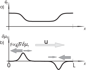
Figure 1: Equilibrium distribution of the spin density ${\rho_{0}}_{\uparrow}$ along the ring of length $L$ (Fig.1a). When electrons drift into the right (see Fig. 1b) the non-equilibrium spin-up potential $\delta\mu_{\uparrow}$ appears in the regions where the spin-up density ${\rho_{0}}_{\uparrow}$ varies. The total force is a sum of all forces acting on electrons and it is directed to the left. Consequently, it leads to the change of the drift direction.

Spin pendulum. Let us discuss the oscillation process described by Eqs. (Dynamics of Spin-Polarized Electron Liquid and Spin Pendulum-Dynamics of Spin-Polarized Electron Liquid and Spin Pendulum) which is related to the current $I=I_{0}e^{i\omega t}$, i.e. a spin pendulum. In the linear approximation we may solve the problem completely and find the frequency of the oscillations

$$\omega^{2}={\displaystyle\oint{\left(\frac{\rho_{\uparrow}}{\rho}\right)^{\prime}}^{2}\frac{1}{\Pi^{*}}dx}\left(\displaystyle\oint\frac{m}{\rho}dx\right)^{-1},\;\frac{\displaystyle 1}{\displaystyle\Pi^{*}}=\sum\limits_{\sigma}\frac{\displaystyle 1}{\displaystyle\Pi_{\sigma}}.$$ (6)

$$u=\frac{\displaystyle I}{\displaystyle es\rho},\quad\delta\mu_{\sigma}=i\frac{\displaystyle I}{\displaystyle es\omega\Pi_{\sigma}}\left(\frac{\displaystyle\rho_{\sigma}}{\displaystyle\rho}\right)^{\prime},$$ (7)

$$\quad e\varphi^{\prime}=-\frac{i}{\omega es}\left[\frac{\displaystyle m\omega^{2}}{\displaystyle\rho}+\sum\limits_{\sigma}\frac{\displaystyle\rho_{\sigma}}{\displaystyle\rho}\left(\frac{\displaystyle 1}{\displaystyle\Pi_{\sigma}}\left(\frac{\displaystyle\rho_{\sigma}}{\displaystyle\rho}\right)^{\prime}\right)^{\prime}\right]I$$

Here $x$ is the coordinate along the conducting channel, ”up arrow” corresponds to the one of spin components; $s$ is the cross-section of the channel which is assumed $x$-independent; strike denotes differentiation with respect to $x$, $L$ is the length of the conducting channel (i.e. the ring length, in our case).

As is evident from Eqs.(6-7), the oscillations exist only when the relative concentration of the spin components varies along the channel. The frequency of oscillations is proportional to the level of the magnetic inhomogeneity, $\alpha=({\rho_{\sigma}}_{max}-{\rho_{\sigma}}_{min})/\rho$, viz.

$$\omega\approx\alpha{\displaystyle v_{F}}{\displaystyle(LL_{1})}^{-1},$$ (8)

where $L_{1}$ is the characteristic scale of the spectrum inhomogeneity.

Initially, the oscillations of the spin-pendulum could be exited by the ”magnetic push” when an external magnetic field is switched on (much faster than $\omega^{-1}$) and an initial current $I=es\Phi/cm$ is induced (where $\Phi$ is the magnetic flux through the ring). Naturally, there are dissipation processes in the hydrodynamic flow, which we did not take into account. They lead to the damping of the spin-pendulum oscillations. It is easy to estimate the decay time

$$\tau_{d}\approx\left(\frac{e^{2}\rho sR}{mL}+\frac{D}{L_{1}^{2}}+\frac{1}{\tau_{sf}}\right)^{-1},$$ (9)

where $R$ is the electrical resistance of the homogeneous ring. The second term in the r.h.s. of Eq.(9) is related to the diffusion of the nonequilibrium spins through the inhomogeneous region. In the hydrodynamic regime the diffusion coefficient is determined by the normal collisions, i.e. $D\approx l_{N}v_{F}$. The third term in the r.h.s. of Eq.(9) corresponds the spin relaxation which is due to the spin-flip with the characteristic time $\tau_{sf}$. Note, as it follows from Eq.(9), the ”space-sharp” inhomogeneity (e.g., a sharp interface boundary between different magnetic materials) causes a very fast decay of the oscillations.

It seems interesting that there exists a possibility to keep the amplitude of the oscillations constant (like in an ordinary pendulum clock) owing to the magnetic connection of the ring with an energy-pumping cell.

Spin-electrical effect. Let us discuss now a spin-electrical effect in an open-ended homogeneous conductor. At ${\mathbf{u}}=0$ we obtain from Eqs. (4) - (7) the following potential difference between the open ends

$$\varphi(L) -\varphi(0)=\frac{e}{\rho}[P(0)-P(L)],$$ (10)

$$P(x) =\left(\rho_{\uparrow}-\frac{\rho_{\downarrow}\Pi_{\uparrow}}{\Pi_{\downarrow}}\right)\delta\mu_{\uparrow}+\left(\Pi_{\uparrow}-\frac{\rho_{\uparrow}}{\Pi_{\uparrow}}\frac{\partial\Pi_{\uparrow}}{\partial\mu_{\uparrow}}\right)\delta\mu_{\uparrow}^{2}+...$$ (11)

Eq. (11) yields the electron pressure as the expansion in series on the $\delta\mu$. The second order term is written in the form for the case of non-magnetic materials. All the quantities in the coefficients of $\delta\mu_{\uparrow}$ and $(\delta\mu_{\uparrow})^{2}$ are understood as the equilibrium state quantities. It is obvious from Eq.(10) that the difference between the non-equilibrium spin pressures at the ends of the circuit induces an electrical voltage that can be measured experimentally. The voltage exists during the lifetime $\tau_{\varphi}$ which is determined either by the spin relaxation due to the spin-flip processes or by the diffusion equalization of the spin concentration along the circuit, $\tau_{\varphi}\approx(\tau_{sf}^{-1}+D/L^{2})^{-1}$. The electrical charge $q\approx\Delta\varphi\tau_{\varphi}$ flows through the meter during this time. Let us discuss the case when the spin polarization is induced in a non-magnetic conductor due to the current spin injection from the magnetic material. Then, a voltmeter connected to the ends of the non-magnetic conductor will fix the electrical charge $q$ and indicate the non-equilibrium spin density be existed in the non-magnetic conductor.

We should note here that this ”spin-electrical” effect is not a specifically hydrodynamic effect. In the diffusion regime, when collisions that do not conserve momenta are dominated over normal collisions, we may write the continuity equations in the following form

$$\frac{\displaystyle\partial\delta\rho_{\sigma}}{\displaystyle\partial t}+\mathrm{div}\sigma_{\sigma}(\nabla(\delta\mu_{\sigma}+e\varphi))=0,$$ (12)

where $\sigma_{\sigma}$ is the contribution to the conductivity of the corresponding spin component, $\sigma=\sum\limits_{\sigma}\sigma_{\sigma}$. Consequently, taking into account Eq.(Dynamics of Spin-Polarized Electron Liquid and Spin Pendulum) we obtain the following equation for the case of homogeneous conductor

$$e\varphi(x)=\left(\frac{\sigma_{\downarrow}\Pi_{\uparrow}}{\Pi_{\downarrow}}-\sigma_{\uparrow}\right)\frac{\delta\mu_{\uparrow}}{\sigma}+\\ \left(\frac{\sigma_{\uparrow}}{\Pi_{\uparrow}}\frac{\partial\Pi_{\uparrow}}{\partial\mu_{\uparrow}}-\frac{\partial\sigma_{\uparrow}}{\partial\mu_{\uparrow}}\right)\frac{\delta\mu_{\uparrow}^{2}}{\sigma}+\ldots$$ (13)

Here, the second term in the r.h.s. of Eq.(19) is written for the case of non-magnetic conductors only.

Conclusion. In summary, the low-decay oscillations of the spin polarization with the frequency $\omega$ accompanied by the oscillations of the drift current may be induced in the conducting ring with inhomogeneous magnetic properties under the condition $\tau_{N}<<\omega^{-1}<<\tau_{d}$ (see Eq.(6, 9). In the case of the heterostructures, the inhomogeneity may be induced by the inhomogeneous Rashba splitting due to the space-dependent electrical field. Assuming that the splitting $\Delta p_{F}$ is small enough, i.e. $\Delta p_{F}/p_{F}<<1$, we obtain from Eq.(9) that $\omega=v_{F}[\frac{2}{L}\oint{(\frac{\Delta p_{F}}{p_{F}})^{\prime}}^{2}dx]^{1/2}$. In the case of a completely nonmagnetic and inhomogeneous ring the excitation of local spin polarization also induces non-linear ”spin-pendulum-like” oscillations, but the consideration of that goes beyond the framework of this paper. In the case of the open circuit, one may detect a non-equilibrium spin-polarization, measuring the voltage between the open ends of the circuit. It can be done both in the hydrodynamic and diffusion regimes.

Acknowledgements. The work was supported in part by NanoProgram of the NAS of Ukraine (Grant No. 3-026/2004) and by the joint Ukraine - Byelorussia Grant No. 10.01.006.

References

- [1] I. Z̆utić, J. Fabian, and S. Das Sarma, Rev. Mod. Phys., 76, 323
- [2] K. Flensberg, T.S. Jensen, N.A.Mortensen, Phys. Rev. B, 64, 245308 (2001). (2004).
- [3] R.N. Gurzhi, A.N. Kalinenko, A.I. Kopeliovich, A.V. Yanovsky, E.N. Bogachek, andUzi Landman, J. Supercond.: Inc. Nov. Magn., 16, 201 (2003).
- [4] R.N. Gurzhi, A.N. Kalinenko, A.I. Kopeliovich, A.V.Yanovsky, E.N. Bogachek, and Uzi Landman, Low Temp.Phys., 29, 606 (2003).
- [5] R.N. Gurzhi, Pis’ma Zh.Eksp.Teor.Fiz., 44, 771 (1963).
- [6] J.H. Davies, ”The Physics of low-dimensional semiconductors”, Cambridge University Press, 438 p., (1997).
- [7] V.A. Buntar’, Yu.Z. Kovdrya, V.N. Grigor’ev, Yu.P. Monarkha, and S.S. Sokolov, Sov. J. Low Temp. Phys. 13, 451, 1987 ]
- [8] M.J.M. de Jong, L.W. Molenkamp. Phys. Rev. B, 49, 5038 (1994); Phys. Rev. B, 51, 13389 (1995).
- [9] R.N. Gurzhi, A.N. Kalinenko, A.I. Kopeliovich, Phys. Rev. Lett., 74, 3872 (1995).
- [10] G.A. Smolenskii, I.E. Chupis, Sov. Phys. Usp. 25, 475, (1982).
- [11] E.I. Rashba, Sov. Phys. - Solid State, 2, 1109 (1960).
- [12] J. Nitta, T. Akazaki, H. Takayanagi, and T. Enoki, Phys. Rev. Lett., 78, 1335 (1997).
- [13] R.N. Gurzhi, V.M. Kontorovich, Zh. Eksp. Teor. Fiz., 55, 1105, 1968.
- [14] R.N. Gurzhi, V.M. Kontorovich, Fiz.Tverd.Tela, 11, 3109, 1969.
- [15] L.D. Landau and E.M. Lifshitz, Hydrodynamics, Pergamon Press, Oxford, 1987.