The CFHTLS-Strong Lensing Legacy Survey (SL2S): Investigating the group-scale lenses with the SARCS sample

Abstract

We present the Strong Lensing Legacy Survey - ARCS (SARCS) sample compiled from the final T0006 data release of the Canada-France-Hawaii Telescope Legacy Survey (CFHTLS) covering a total non-overlapping area of 159 deg². We adopt a semi-automatic method to find gravitational arcs in the survey that makes use of an arc-finding algorithm. The candidate list is pruned by visual inspection and ranking to form the final SARCS sample. This list also includes some serendipitously discovered lens candidates which the automated algorithm did not detect. The SARCS sample consists of 127 lens candidates which span arc radii $\sim 2\arcsec-18\arcsec$ within the unmasked area of $\sim$150 deg². Within the sample, 54 systems are promising lenses amongst which, we find 12 giant arcs (length-to-width ratio $\geq 8$). We also find 2 radial arc candidates in SL2SJ141447+544704. From our sample, we detect a systematic alignment of the giant arcs with the major axis of the baryonic component of the putative lens in concordance with previous studies. This alignment is also observed for all arcs in the sample and does not vary significantly with increasing arc radius. The mean values of the photometric redshift distributions of lenses corresponding to the giant arcs and all arcs sample are at $z\sim 0.6$. Owing to the large area and depth of the CFHTLS, we find the largest sample of lenses probing mass scales that are intermediate to cluster and galaxy lenses for the first time. We compare the observed image separation distribution (ISD) of our arcs with theoretical models. A two-component density profile for the lenses which accounts for both the central galaxy and the dark matter component is required by the data to explain the observed ISD. Unfortunately, current levels of uncertainties and degeneracies accommodate models both with and without adiabatic contraction. We also show the effects of changing parameters of the model that predict the ISD and that a larger lens sample might constrain relations such as the concentration-mass relation, mass-luminosity relation and the faint-end slope of the luminosity function.

1. INTRODUCTION

Gravitational lensing is the deflection of light coming from distant sources in the Universe, due to the gravitational potential of intervening structures (see reviews e.g. Blandford & Narayan, 1986, 1992; Kochanek, 2006). The last decade has seen the rise of a wide variety of applications of strong lensing such as the study of distant lensed galaxies with unprecedented magnification (e.g., Impellizzeri et al., 2008; Swinbank et al., 2009; Zitrin & Broadhurst, 2009; Richard et al., 2011), the constraints on substructure within lensing halos (e.g., More et al., 2009a; Suyu & Halkola, 2010; Vegetti et al., 2010a, b), accurate measurements of the Hubble constant (e.g., Coles, 2008; Suyu et al., 2010), constraints on the stellar initial mass function (e.g., Treu et al., 2010; Ferreras et al., 2010; Sonnenfeld et al., 2011), constraints on the slope of the inner density profile of the lensing halos (e.g., Treu & Koopmans, 2002a, b; Koopmans & Treu, 2003; Koopmans et al., 2006; More et al., 2008; Barnabè et al., 2009; Koopmans et al., 2009) and estimation of the fraction of dark matter in galaxy-scale halos (e.g., Gavazzi et al., 2007; Jiang & Kochanek, 2007; Grillo et al., 2010; , 2011; More et al., 2011a; Ruff et al., 2011).

Although strong lensing is a rare event, several surveys covering a wide sky area and deep enough imaging across different wavelengths, have resulted in the discovery of over 200 strong lens systems at galaxy scales from surveys such as, the Great Observatories Origins Deep Survey (, 2004), Cosmic Evolution Survey (COSMOS Faure et al., 2008; Jackson, 2008), Mediu Deep Survey (Ratnatunga et al., 1999) the Cosmic Lens All Sky Survey (CLASS, Myers et al., 2003) and the Sloan Lens ACS Survey (SLACS, Bolton et al., 2006) and about a few dozen lens systems at cluster scales such as, the Extended Medium Sensitivity Survey (EMSS, Luppino et al., 1999), the MAssive Cluster Survey (MACS, Ebeling et al., 2001), the Las Campanas Distant Cluster Survey (LCDCS, Zaritsky & Gonzalez, 2003) and the Red sequence Cluster Survey (RCS, Gladders et al., 2003, henceforth G03). Large imaging and spectroscopic surveys enable us to probe statistical properties of both dark matter and baryonic matter or constrain cosmological parameters with high accuracy. For instance, on galaxy scales, the SLACS sample has been used to study the average density profiles of lens galaxies up to redshift of $\sim$0.3 (e.g., Koopmans et al., 2006; Gavazzi et al., 2007; Koopmans et al., 2009; Auger et al., 2010), Falco et al. (1999) used the CfA-Arizona Space Telescope LEns Survey (CASTLES, Muñoz et al., 1998) sample to measure the mean extinction due to the interstellar medium of the lens galaxies, (2009) estimated the fraction of mass in compact objects within lens galaxies from the CASTLES, Wyithe (2004) constrained the bright end of the quasar luminosity function from the absence of lensed quasars at high redshift in the Sloan Digital Sky Survey (SDSS). On cluster scales, G03 found the observed abundance of giant arcs from the RCS is too high to be consistent with the predictions from the current standard cosmological model (see also Bartelmann et al., 1998; Li et al., 2005, 2006) and Zitrin et al. (2011) found some discrepancy between the predictions from the standard model and the observed distribution of Einstein radii from the MACS sample. However, the magnitude of these differences has been mitigated with subsequent studies (e.g., Horesh et al., 2005; Meneghetti et al., 2011).

As discussed above, the majority of the surveys in the past have primarily focused on studying galaxy-scale or cluster-scale structures. As a result, matter distribution in galaxies and galaxy clusters is relatively well-studied via both strong and weak lensing. A further improvement in our understanding has come from the use of complementary methods to lensing such as stellar kinematics, satellite kinematics and X-ray scaling relations. In contrast, little is known about galaxy groups which are intermediate to galaxies and galaxy clusters, typically corresponding to masses of $10^{12}-10^{14}~{}M_{\odot}$. Relatively fewer investigations have been carried out with galaxy groups e.g., study of intra-group medium with very low redshift X-ray sample (Helsdon & Ponman, 2000), study of mass-to-light ratios with the Canadian Network for Observational Cosmology 2 sample (Parker et al., 2005), study of faint end of the luminosity function of nearby compact groups (Krusch et al., 2006), study of concentration-mass ($c$-$M$) relation from the SDSS (Mandelbaum et al., 2008) via weak lensing, study of colors and star formation (e.g., Balogh et al., 2009, 2011), study of scaling relations of X-ray selected groups (Rines & Diaferio, 2010) and study of baryon fractions from the 2MASS (Dai et al., 2010). Since studies of groups are limited and we still do not have a detailed understanding of matter distribution, formation and evolution of galaxy groups. Being one of the important components in the hierarchical assembly of structures in the Universe, galaxy groups are much more massive than galaxy-scale halos and are concentrated enough to act as lenses. Furthermore, since galaxy groups are quite abundant compared to massive structures like galaxy clusters, the probability to find group scale lenses is also large. Hence, lensing can be successfully used to study group-scale halos.

The Strong Lensing Legacy Survey (SL2S, Cabanac et al., 2007) is a survey from the Canada-France-Hawaii Telescope Legacy Survey (CFHTLS). The design of the CFHTLS allows us to find large sample of group-scale lenses, which can be studied in detail upto high redshifts, for the first time. The SL2S is as a precursor to wide field imaging surveys such as the Dark Energy Survey, Large Synoptic Survey Telescope and Euclid. A combined study of SL2S galaxy-scale lenses with the SLACS sample have been used to show mild evolution of the slope of the average density profile of galaxies (Ruff et al., 2011) which is constrained by the strong lensing and stellar dynamics techniques. Disk galaxies are also a relatively less studied population especially at high redshifts. An automated search for edge-on disk lenses from the SL2S resulted in 18 candidates , out of which 3-5 are expected to be real lenses (Sygnet et al., 2010). A subset of the SL2S groups have been studied in detail using a combination of techniques such as strong lensing, group dynamics, weak lensing to probe the density profiles of the lensing groups (e.g., Limousin et al., 2009; Thanjavur et al., 2010; Verdugo et al., 2011).

In this paper, we present the SL2S-ARCS sample from the final T0006 release of the CFHTLS. In Section 2, we give an overview of the survey and procedure of sample selection, describe details of the algorithm, arcfinder (Alard, 2006) and present the final sample. In Section 3, we discuss some statistical results using the final sample. In Section 4, we summarize the survey and our main findings.

2. THE CFHTLS-SL2S ARCS SAMPLE

In this section, we give a brief overview of the survey from which we derive the lens sample. This is followed by a description of the semi-automatic process of selecting the candidates in the final sample. We also discuss how the algorithm, arcfinder works and the modifications implemented in the new arcfinder. Lastly, we present the final sample and report duplicate detections of some candidates from other surveys.

2.1. Survey Overview

CFHTLS is a photometric survey made with the Canada-France-Hawaii Telescope (CFHT) in five optical bands ($u^{*}g^{\prime}r^{\prime}i^{\prime}z^{\prime}$) using the wide-field imager MegaPrime with a field-of-view of 1 deg² on the sky and a pixel size of 0.186″. The WIDE and DEEP components of the CFHTLS are designed to carry out extragalactic research. These components are ideal for searching strong lens systems. The SL2S sample is compiled from the CFHTLS-WIDE encompassing a combined area of 171 deg² and CFHTLS-DEEP encompassing a combined area of 4 deg². However, taking into account the masked and overlapping areas, the effective area of the survey is 150.4 deg² (146.9 deg² for WIDE and 3.5 deg² for DEEP). The WIDE consists of four fields W1, W2, W3 and W4. The field W1 has the largest sky coverage of 63.65 deg². The fields W2 and W4 have similar sky coverages of 20.32 deg² and 20.02 deg², respectively. The field W3 has a sky coverage of 42.87 deg² and is more than twice as large as W2 and W4. The DEEP also consists of four fields D1 (located within the W1 field), D2, D3 and D4. Each of the deep fields covers an area of 1 deg². The DEEP images are produced in two image stacks D-25 and D-85. The former consists of 25% of the best seeing images and the latter consists of 85% of best seeing images. We use the D-25 images for searching lens candidates. Among the WIDE fields, $g$ band imaging is the deepest of all bands with a limiting magnitude of 25.47 and a mean seeing of 0.78″ whereas the $g$ band imaging of DEEP fields has nearly 10 times deeper exposures than the WIDE fields and the median seeing is $\sim 0.7\arcsec$. The zero point to convert flux to AB magnitude for all bands is 30. Further details of the T0006 release, which is the first complete release of the WIDE and DEEP, can be found on Terapix website.

2.2. Sample selection

The SL2S lens sample is compiled using two algorithms: ringfinder and arcfinder. The former aims at detecting galaxy-scale lenses by using color information. The SL2S RINGS sample will be presented and discussed in a separate paper (Gavazzi et al., in preparation). Here, we focus on the SL2S-ARCS (SARCS) sample created with the help of arcfinder, followed by visual inspection and screening of the candidates.

We define the SARCS sample such that lens systems with arc radius ($R_{\rm A}$) $\gtrsim 2\arcsec$ belong to the sample. The radius of the arc is defined as the distance of the lensed image from the putative lens galaxy which is roughly the Einstein radius. Typically, lensing halos with Einstein radius larger than 2″are very massive lenses with significant contribution from the environment of the primary lensing galaxy. Thus, the SARCS sample, predominantly, consists of group to cluster scale lenses. Lens systems with $R_{\rm A}<2\arcsec$, typically, form part of the RINGS sample. We note that a few lens systems are common to both SL2S samples since the cut on $R_{\rm A}$ is not a sharp limit imposed by the algorithms.

The SARCS sample from the CFHTLS is compiled in a three-step process. The first step is to run the arc-detection algorithm called arcfinder. We choose to run the arcfinder on the $g$-band image since most of the lensed images correspond to galaxies with high star formation that have little emission at redder wavelengths. Also, focusing on g-band prevents from detecting high redshift g-dropouts. However, we plan to search for g-dropout arcs which are brighter in the $i$ band. These results will be presented in a separate paper.

At the end of the first step, we produce a list of arc candidates with various parameters. The next step is applying a cut-off on arc properties such as the area, the peak flux count, the radius of curvature and reject candidates within masked area. These cuts allow a significant reduction in false detections at the cost of losing some real arc candidates. In the third step, visual inspection and classification are carried out to grade the quality of the candidates. Note that the final SARCS sample consists of candidates that are detected by the arcfinder and/or by visual inspection.

2.3. Automatic detection of arcs: arcfinder

With the advent of several large imaging surveys, searching for lens systems visually is a subjective and time expensive exercise which may not be easily repeatable. Hence, several algorithms have been devised in the last few years to automate the process of lens detection as much as possible. The algorithms, usually, focus on a specific target population, for example, algorithms to detect the lensed sources such as quasars via the quasar time variability (Kochanek et al., 2006) based on the difference imaging technique of Alard & Lupton (1998), spectrum-based algorithms such as the one used by Bolton et al. (2004) to form the SLACS sample following the technique of Warren et al. (1996) or lens-modelling robots that assesses the probability of a bright red galaxy being a lens (Marshall et al., 2009). Since groups to cluster scale lenses form arc-like lensed images, there are a few arc-finders in the literature (e.g., Lenzen et al., 2004; Horesh et al., 2005; Seidel & Bartelmann, 2007) that aim at detecting elongated arc-like images.

The arcfinder (Alard, 2006) is a generic algorithm that can be used to detect elongated and curved features in an image. The algorithm uses pixel intensities from a standard FITS image to trace the structure of a feature. Multiple thresholds are applied to the structural properties of the feature to select an arc candidate. The reader is referred to Alard (2006) for the details of the algorithm. Below, we describe the algorithm along with some modifications implemented in the newer version (V2.0) which is used to compile the SARCS sample.

Figure 1.— Flowchart showing the arcfinder algorithm.

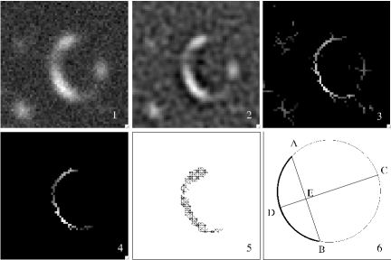
Figure 2.— Outputs of arcfinder at various stages of the execution (panels 1-5) using a mock arc image. Panel 1 - original image with the mock arc, panel 2 - smoothed image, panel 3 - (disconnected) pixels with elongation estimator values higher than a threshold, panel 4 - connected pixels above thresholds that belong to the arc and panel 5 - the reconstructed shape of the final arc. The image is 11.3″on the side. Schematic diagram for measuring length of an arc (panel 6).

We show a flowchart to illustrate the various steps involved in the algorithm (see Fig. 1) and step through an example of a mock arc image (see Fig. 2).

• We run the arcfinder on images of 19354$\times$19354 pixels which corresponds to a single MEGACAM pointing. For such large images, the assumption of Gaussian distribution for the noise holds well. Assuming a Gaussian distribution for the noise in the input image (panel 1 of Fig. 2), the noise $\sigma$ is calculated in the first step. Most of the arcs are unresolved with the ground-based telescopes like CFHT and are limited by the size of the point spread function (PSF).

• Convolving the image with a smoothing kernel, with a size of the order of the PSF, can help damp the noise and enhance the detection of arcs. Hence, the input image is smoothed with a Mexican-hat filter in the next step (panel 2 of Fig. 2).

  The Mexican-hat band-pass filter with scale $b$ is given by

  $$M(x,y)=e^{-\bar{r}^{2}}-0.5e^{-\frac{\bar{r}^{2}}{2}}\,,$$ (1)

  where $b^{2}=3$ pixels and

  $$\bar{r}=\frac{\sqrt{x^{2}+y^{2}}}{b}\,.$$ (2)

• Now, we define a local estimator of elongation for every pixel in the smoothed image. This is calculated by using the flux from all pixels within a window centered on every pixel. The size of the window is chosen to be a few times the PSF size. We consider a square window of side W centered on the pixel at (x,y). Using the second order moments of brightness distribution within the window, the local direction of the elongation of the feature is calculated. This direction is then used to align the feature along the x-axis to determine the local axis ratio, similar to a length-to-width ratio, within the window. The elongation estimator is defined as follows

  $$Q(x,y)=\frac{1}{W}\frac{F_{\rm X}}{F_{\rm Y_{\rm max}}}\,,$$ (3)

  where $F_{\rm X}$ is the integrated flux of the single central row of pixels and $F_{\rm Y_{\rm max}}$ is the maximum of the integrated flux values calculated from single columns of pixels within the window. If $F_{\rm X}$ and $F_{\rm Y_{\rm max}}$ are above $(W+1)0.75\sigma$ (threshold 1 in Fig. 1 and Table 1), then the estimator $Q(x,y)$ is assigned to the pixel (x,y) at the center of the window else the pixel is assigned a value of 0. Likewise, the estimator is calculated for every pixel in the image (see panel 3 of Fig. 2).

  Table 1 Thresholds used in the final selection of the SARCS candidates.

  Step	Parameters and Thresholds
  Smooth	W=9, $b^{2}=3.0$
  Detect	W=11, Th1=11*0.75$\sigma$
  Connect	W=9, Th2=1.25
  	W=9, Th4=0.5S1,0.3S2
  Properties	Final Thresholds
  Area	$55<~{}{\rm A}~{}<500$ (pix)
  peak counts	$<50$ (ADU s-1)
  mean counts	$2\sigma<~{}{\rm SB}~{}<50$ (ADU s-1 pix-1)
  length	$>7$ (pix)
  width	$1.5\leq~{}{\rm w}~{}\leq 8$ (pix)
  curvature	$r_{c}<100$ and $r_{c}>1000$ (pix)

• In the following step, we attempt to connect the pixels that possibly belong to the candidate arc. A pixel is accepted if the estimator value from the image in panel 3 is $>1.25$ (threshold 2 in Fig. 1 and Table 1). The estimator is set to 0 as soon as a pixel is connected in the prior step to avoid repetitive checking of connected pixels. Iterating the above steps over the image allows tracing of the primary shape of the arc. If the number of connected pixels is more than 10 (threshold 3) then the properties of arcs such as the length, peak flux and surface brightness are calculated. The panel 4 shows the image with connected pixels which, for the case at hand, consists of one candidate only. The estimator is particularly suited for recovering pixels along the length of the arc. In order to connect the pixels along the width of the arc, we use the input and smoothed images (panels 1 and 2, respectively). Using arcs with length $>7$ pixels, we apply surface brightness thresholds on pixel values from images in panels 1 and 2 in order to accept pixels belonging to the arc (threshold 4, see Fig. 1 and Table 1) and construct the arc fully.

• In the last step, if the candidate arc satisfies thresholds on the arc properties such as the width ($\geq 1.5$ and $\leq$8 pixels), area ($>25$ pixels), surface brightness ($>2\sigma$) and peak flux ($<500$ ADU/s/pixel) which correspond to threshold 5 in Fig. 1, then the arc is accepted (see panel 5 in Fig. 2).

• In the following, we describe how the arc properties are measured. The area of the arc is the total number of pixels belonging to the final arc. The length of the arc is calculated by assuming that the candidate arc is similar to an arc of a circle. We first find the extreme ends of the arc, connect them with a chord labeled AB in the panel 6 of Fig. 2. From the midpoint E of chord AB, we draw a line perpendicular to the chord and find its intersection D with the arc. The lengths ED and AB uniquely identify the circle to which the arc belongs and as well as the length of the arc. The width of the arc is defined as the ratio of the area to the length of the arc. The radius of the circle going through the arc is used as a proxy for the curvature of the arc.

In the algorithm, the use of a second image at another wavelength and a mask file are optional. The algorithm, in its current version, merely prints the values of the pixels belonging to the candidate arc from the image 2 and/or the mask file, if provided. This allows us to optionally screen the candidate arcs based on their color and/or masking information. For the SARCS sample, we made use of the mask option only and further restricted the parameter space of the output list of arcs by introducing more strict cuts on some of the arc properties. The Table 1 lists the final set of thresholds which are satisfied by the SARCS candidates detected by arcfinder.

The components enclosed by the dashed line in the Fig. 1 are the sections of the algorithm that have been improved. This includes the way in which the pixels belonging to the arc are connected and the way the properties of the arcs are measured. In the earlier version of the algorithm, a candidate arc is accepted at the final stage only if it satisfies a certain threshold on the curvature of the arc. This feature has been removed and the option of using mask information is introduced in the V2.0. The values for all the different thresholds are tuned from an initial sample of CFHTLS arcs, found visually or from the previous version of arcfinder, based on an early release of the data. Furthermore, all the thresholds can now be set during the execution of the algorithm.

The arcfinder V2.0 finds $\sim 1.5\times$ more detections, most of which arise due to spikes and halos near stars. However, the use of masks removes these false detections thereby making the number of detections comparable or less than the output of the earlier version. The modified arcfinder is over 3 times faster than the earlier version. We have also recently parallelized the algorithm which enables us to achieve even faster computation on shared memory platforms. The arcfinder V2.0 is available upon request to the author.

Finally, we note that the existing algorithms are far from perfect and almost always require manual intervention. Attempts to increase the completeness of the sample almost always leads to a corresponding increase in the rate of false positives. In light of these issues, citizen science projects such as the Galaxy Zoo (Lintott et al., 2008) might be a better tool, for the time being, in identifying lens systems not detected by the algorithms. These projects, in turn, could be used to calibrate and improve existing algorithms. We are currently pursuing the feasibility of such a project.

2.4. SARCS sample

After the automatic detection and screening, about 1000 candidates/deg² are visually inspected. This is reduced to a total sample of 413 candidates which is further considered for ranking by three people. The individually assigned ranks are from 1 to 4 with 1 being the least likely to 4 being the almost certain lens system. We present the 127 lens candidates which are ranked 2 or higher (average of the ranks by three people) and which have $R_{\rm A}\gtrsim 2\arcsec$. All of the 127 candidates are listed in Table LABEL:tab:all that gives the ID, lens position, lens magnitudes in AB, lens redshifts with 1$\sigma$ uncertainties, arc radii, ranks, the type indicating whether the candidates are primarily detected via the arcfinder and the field name in which the candidate is located. For the calculation of arc radii in physical units, we use flat cosmology with following parameters ($\Omega_{m},\Omega_{\Lambda},H_{0}$)=(0.3,0.7,100 km s^-1 Mpc^-1). The symbol A stands for detection by arcfinder and V implies candidate is found serendipitously. A total of 54 candidates are good to best systems (that is, rank of 3 and above) and are shown in the Fig. 3 and Fig. 4. Out of the total sample, 27 systems have been or are being followed up for further analyses (see Table 3) and most of them are confirmed lens systems, 5 systems are very likely lenses and rest of the 96 are possible lenses. The Table 3 does not report information about any archival data on any of the lens candidates.

One of the deep fields, D2, has an overlap with the COSMOS (Scoville et al., 2007), a photometric survey of 1.8 deg² in the $I$ band (limiting magnitude of 26.5) with the Advanced Camera Survey (ACS) on HST. We find two of the SARCS candidates common to the lens sample of COSMOS (Faure et al., 2008). The SARCS candidates with IDs SA78 and SA83 are known COSMOS candidates and the rest of the 6 candidates within the COSMOS field are new (see Table LABEL:tab:all with Field labelled as D2). For comparison, we also show the ACS images of the SARCS candidates in Fig. 5 from the COSMOS archive. The W3 field overlaps with one of the 22 individual fields of the RCS survey which covers a combined area of $\sim$90 deg². The overlapping RCS field has a lensing cluster, RCS 1419.2+5326 at $z=0.64$. This cluster is also detected in the SARCS sample identified by SA102 (see Table LABEL:tab:all).

Table 2 Characteristics of lens candidates from the SARCS sample.

ID	RA	Dec	$g$	$r$	$i$	$z_{\rm phot}$	$R_{\rm A}$		Rank	Type	Field
	hms	dms	mag	mag	mag		″	$h^{-1}$Kpc
SA1	02:01:21.89	$-$09:15:15.09	22.06	20.58	19.90	0.46$\pm$0.02	2.2	9.0	2.0	A	W1
SA2	02:02:10.50	$-$11:09:11.68	19.79	18.48	17.80	0.48$\pm$0.02	5.0	20.9	3.7	A	W1
SA3	02:02:38.87	$-$06:34:56.12	20.89	19.91	19.54	0.37$\pm$0.03	2.2	7.9	2.0	A	W1
SA4	02:03:02.84	$-$08:21:14.25	21.96	20.57	19.99	0.14$\pm$0.07	2.4	4.1	2.0	V	W1
SA5	02:03:12.61	$-$10:47:07.95	22.02	20.55	19.52	0.62$\pm$0.03	3.0	14.3	2.3	V	W1
SA6	02:03:20.43	$-$07:34:50.78	21.69	20.36	19.45	0.59$\pm$0.03	5.0	23.2	3.3	A	W1
SA7m	02:03:49.98	$-$09:42:53.51	17.84	16.73	16.18	0.25$\pm$0.02	5.0	13.7	3.3	A	W1
SA8	02:04:54.51	$-$10:24:02.48	19.52	18.18	17.68	0.33$\pm$0.02	10.8	35.9	2.7	A	W1
SA9	02:05:03.15	$-$11:05:46.63	21.54	20.17	19.16	0.62$\pm$0.03	3.3	15.7	3.0	V	W1
SA10	02:06:48.47	$-$06:57:01.33	20.95	19.60	18.90	0.49$\pm$0.06	3.2	13.5	3.0	A	W1
SA11	02:08:15.66	$-$07:24:57.81	21.98	20.55	19.49	0.62$\pm$0.02	4.3	20.4	2.0	A	W1
SA12	02:08:16.87	$-$09:36:52.69	22.16	20.85	19.60	0.74$\pm$0.03	3.4	17.4	3.7	A	W1
SA13	02:08:41.61	$-$07:01:28.07	19.85	18.70	18.20	0.29$\pm$0.03	3.5	10.7	2.0	V	W1
SA14	02:09:29.33	$-$06:43:11.26	20.47	19.15	18.57	0.45$\pm$0.02	3.2	12.9	3.7	A	W1
SA15	02:09:57.67	$-$03:54:57.08	21.41	19.98	19.27	0.43$\pm$0.03	3.9	15.3	2.3	V	W1
SA16	02:10:26.57	$-$04:46:41.59	21.77	20.79	20.24	0.55$\pm$0.03	1.9	8.5	2.0	A	W1
SA17	02:10:51.59	$-$03:52:52.64	21.79	20.84	19.91	0.73$\pm$0.04	1.9	9.7	2.0	V	W1
SA18	02:11:08.66	$-$10:12:13.86	19.81	18.44	17.89	0.38$\pm$0.02	2.0	7.3	2.3	A	W1
SA19	02:11:18.49	$-$04:27:29.20	23.13	22.48	21.43	1.19$\pm$0.07	3.5	20.3	3.3	A	W1
SA20	02:12:20.52	$-$09:38:44.10	23.48	22.18	20.88	0.77$\pm$0.03	2.4	12.4	2.0	A	W1
SA21G	02:13:24.52	$-$07:43:54.82	24.11	23.73	23.18	0.80$\pm$0.16	2.8	14.7	4.0	V	W1
SA22	02:14:08.07	$-$05:35:32.39	20.98	19.42	18.69	0.48$\pm$0.02	7.1	29.7	4.0	A	W1
SA23G	02:14:11.24	$-$04:05:02.71	22.11	20.92	19.88	0.74$\pm$0.04	1.9	9.7	4.0	A	W1
SA24	02:15:23.03	$-$07:36:23.56	23.64	22.08	20.89	1.05$\pm$0.02	3.7	21.0	2.7	A	W1
SA25	02:15:52.36	$-$07:21:01.32	21.50	20.06	19.29	0.48$\pm$0.02	2.8	11.7	2.0	A	W1
SA26m	02:16:04.66	$-$09:35:06.65	21.68	20.26	19.09	0.69$\pm$0.02	16.4	81.6	2.7	V	W1
SA27mG	02:16:24.03	$-$09:57:39.09	17.29	16.35	15.90	0.18$\pm$0.02	2.8	5.9	3.3	A	W1
SA28	02:16:31.19	$-$07:31:57.13	21.90	20.89	19.80	0.86$\pm$0.04	2.4	12.9	2.3	A	W1
SA29	02:16:46.84	$-$09:18:16.74	21.73	20.53	19.48	0.72$\pm$0.03	2.4	12.1	2.5	V	W1
SA30	02:16:49.25	$-$07:03:23.80	21.04	19.54	18.85	0.45$\pm$0.02	5.6	22.6	3.7	A	W1
SA31m	02:17:23.76	$-$10:15:50.30	18.68	17.53	17.03	0.27$\pm$0.02	3.2	9.3	2.3	V	W1
SA32	02:17:39.56	$-$10:33:19.93	22.94	22.05	21.04	1.05$\pm$0.05	1.9	10.8	2.3	A	W1
SA33m	02:18:07.29	$-$05:15:36.16	22.54	21.21	20.18	0.42$\pm$0.03	2.4	9.3	3.7	V	W1
SA34	02:18:14.39	$-$10:06:02.30	21.20	20.57	20.27	0.46$\pm$0.03	2.8	11.4	2.0	A	W1
SA35	02:19:09.86	$-$04:01:43.32	21.43	19.95	19.27	0.45$\pm$0.02	4.3	17.3	2.3	A	W1
SA36	02:19:56.42	$-$05:27:59.21	20.48	19.38	18.84	0.35$\pm$0.04	3.0	10.4	3.0	V	W1
SA37	02:20:43.11	$-$10:52:16.45	22.81	21.68	20.48	0.79$\pm$0.03	2.2	11.5	2.7	A	W1
SA38	02:20:56.43	$-$07:43:11.71	22.91	21.56	20.51	0.71$\pm$0.03	2.4	12.1	2.3	A	W1
SA39	02:21:51.18	$-$06:47:32.66	21.34	20.18	19.16	0.72$\pm$0.03	5.2	26.3	4.0	V	W1
SA40	02:23:15.41	$-$06:29:06.40	21.20	20.02	19.21	0.55$\pm$0.06	1.9	8.5	3.0	A	W1
SA41	02:23:18.33	$-$10:58:48.46	21.57	20.29	19.53	0.52$\pm$0.04	6.1	26.6	2.0	A	W1
SA42	02:24:00.92	$-$03:46:25.83	23.12	22.04	20.92	0.98$\pm$0.05	2.6	14.5	2.7	A	W1
SA43	02:24:05.01	$-$04:47:07.00	20.00	18.68	18.10	0.36$\pm$0.04	4.3	15.1	2.0	A	D1
SA44	02:24:34.96	$-$04:11:35.02	24.01	23.03	22.06	0.68$\pm$0.04	1.9	9.4	2.7	V	D1
SA45	02:24:35.26	$-$04:01:57.86	22.49	21.21	20.13	1.13$\pm$0.07	3.5	20.1	2.0	V	D1
SA46	02:24:39.06	$-$04:00:45.16	20.75	19.33	18.62	0.43$\pm$0.05	3.2	12.6	3.0	V	D1
SA47	02:24:59.25	$-$04:01:03.77	24.05	22.83	21.70	0.80$\pm$0.04	1.9	10.0	3.0	V	D1
SA48zG	02:25:11.04	$-$04:54:33.54	18.72	17.57	17.03	0.33$\pm$0.01	2.8	9.3	3.7	A	D1
SA49	02:25:38.74	$-$04:03:20.36	22.09	20.64	19.52	0.62$\pm$0.06	4.3	20.4	2.0	A	D1
SA50	02:25:46.13	$-$07:37:38.52	20.99	19.50	18.60	0.54$\pm$0.02	5.8	25.8	4.0	V	W1
SA51	02:26:07.15	$-$04:27:26.26	19.36	18.44	17.97	0.17$\pm$0.05	3.7	7.5	2.0	V	D1
SA52	02:27:20.22	$-$07:49:20.19	21.31	19.81	19.00	0.53$\pm$0.03	2.1	9.3	2.0	V	W1
SA53	02:27:59.21	$-$09:07:29.86	20.71	19.87	19.42	0.55$\pm$0.03	3.9	17.5	2.0	A	W1
SA54	02:28:32.05	$-$09:49:45.44	20.25	18.74	18.07	0.45$\pm$0.02	6.3	25.4	2.7	V	W1
SA55	02:29:17.36	$-$05:54:05.54	19.67	18.30	17.73	0.38$\pm$0.03	2.6	9.5	3.0	A	W1
SA56	02:30:39.96	$-$03:50:28.06	22.36	21.89	21.32	0.27$\pm$0.02	2.1	6.1	2.0	A	W1
SA57	02:31:06.46	$-$05:55:04.63	21.68	20.20	19.46	0.52$\pm$0.03	3.7	16.1	2.0	A	W1
SA58	02:32:23.77	$-$08:50:38.37	22.05	20.76	20.09	0.46$\pm$0.04	2.6	10.6	2.0	A	W1
SA59	02:33:07.05	$-$04:38:38.21	21.56	20.66	19.62	0.79$\pm$0.03	1.9	9.9	2.0	A	W1
SA60	02:35:01.61	$-$09:58:32.76	21.78	20.24	19.07	0.70$\pm$0.03	4.7	23.5	2.7	A	W1
SA61	08:48:23.66	$-$04:07:15.29	21.17	19.63	18.85	0.51$\pm$0.02	7.4	32.0	2.7	A	W2
SA62	08:50:07.72	$-$01:23:53.30	22.23	20.92	20.35	0.37$\pm$0.04	3.5	12.5	2.7	A	W2
SA63	08:52:07.18	$-$03:43:16.28	20.91	19.33	18.61	0.48$\pm$0.02	5.0	20.9	3.3	V	W2
SA64	08:52:08.36	$-$04:05:28.36	21.62	20.26	19.59	0.43$\pm$0.03	2.4	9.4	2.0	A	W2
SA65	08:54:25.14	$-$03:14:53.11	24.89	24.53	22.84	0.98$\pm$0.10	1.9	10.6	2.7	A	W2
SA66m	08:54:46.55	$-$01:21:37.08	19.34	17.88	17.28	0.48$\pm$0.11	4.8	20.1	4.0	A	W2
SA67	08:55:59.92	$-$04:09:17.76	21.06	19.60	18.90	0.45$\pm$0.02	2.1	8.5	3.0	A	W2
SA68	08:57:26.91	$-$02:42:26.64	19.91	18.44	17.80	0.42$\pm$0.02	2.8	10.8	2.3	A	W2
SA69	08:57:35.96	$-$01:01:12.55	21.03	20.57	20.29	0.05$\pm$0.23	2.4	1.6	2.3	A	W2
SA70	08:57:49.10	$-$01:13:00.73	19.99	18.81	18.26	0.29$\pm$0.03	3.9	11.9	2.0	A	W2
SA71m	08:58:48.83	$-$02:39:25.79	19.16	18.23	17.83	0.36$\pm$0.10	3.7	13.0	3.0	V	W2
SA72	08:59:14.55	$-$03:45:14.85	22.01	20.75	19.67	0.74$\pm$0.03	4.5	23.0	4.0	A	W2
SA73m	08:59:54.54	$-$01:32:13.39	20.87	19.47	18.85	0.66$\pm$1.06	4.3	21.0	2.0	A	W2
SA74	09:00:50.10	$-$02:30:54.15	20.52	19.23	18.65	0.36$\pm$0.02	3.2	11.3	2.0	V	W2
SA75	09:02:20.42	$-$02:30:57.28	22.76	21.97	21.41	0.63$\pm$0.04	3.0	14.4	2.3	A	W2
SA76G	09:04:07.97	$-$00:59:52.85	22.03	21.18	20.22	0.77$\pm$0.04	2.4	12.4	3.3	A	W2
SA77	09:05:29.75	$-$02:03:17.70	20.94	19.47	18.80	0.42$\pm$0.02	2.4	9.3	2.0	A	W2
SA78C	09:59:39.17	+02:30:43.98	22.72	21.20	19.92	0.74$\pm$0.06	3.2	16.4	3.0	V	D2
SA79	09:59:42.43	+02:29:56.10	23.10	21.64	20.32	0.76$\pm$0.04	3.5	18.1	3.0	V	D2
SA80	09:59:55.98	+02:19:01.79	23.30	22.19	21.06	1.00$\pm$0.04	2.4	13.5	3.3	A	D2
SA81	10:01:33.74	+02:21:35.35	21.96	20.71	20.08	0.69$\pm$0.05	3.0	14.9	2.0	V	D2
SA82	10:01:47.79	+02:22:06.55	22.92	21.44	20.20	0.69$\pm$0.05	3.5	17.4	2.7	V	D2
SA83C	10:02:11.22	+02:11:39.46	23.64	22.02	20.77	0.89$\pm$0.05	2.6	14.1	4.0	V	D2
SA84	10:02:11.67	+02:29:55.24	22.81	21.55	20.56	0.77$\pm$0.05	1.9	9.9	3.0	A	D2
SA85	10:02:14.85	+02:37:36.47	23.51	22.20	21.15	0.65$\pm$0.05	2.1	10.2	3.0	V	D2
SA86	13:56:49.33	+55:27:07.00	20.41	18.86	18.21	0.46$\pm$0.03	3.7	15.1	2.5	A	W3
SA87	13:57:25.48	+53:17:43.96	20.52	19.03	18.15	0.54$\pm$0.02	3.5	15.6	3.0	A	W3
SA88	13:59:47.26	+55:35:37.57	23.40	22.63	21.57	0.87$\pm$0.04	2.2	11.9	2.3	A	W3
SA89	14:00:40.17	+56:07:49.41	20.47	19.08	18.48	0.42$\pm$0.03	3.7	14.3	3.0	A	W3
SA90	14:01:10.46	+56:54:20.51	20.89	19.42	18.57	0.53$\pm$0.03	3.7	16.3	3.7	A	W3
SA91	14:01:44.90	+53:02:09.62	22.01	20.50	19.61	0.56$\pm$0.03	3.0	13.6	3.7	A	W3
SA92G	14:01:56.39	+55:44:46.78	20.79	19.40	18.70	0.50$\pm$0.03	2.8	12.0	2.0	V	W3
SA93	14:02:47.90	+57:08:52.04	23.70	22.75	21.68	1.22$\pm$0.04	3.2	18.6	2.0	A	W3
SA94	14:03:51.68	+57:23:50.41	24.08	22.48	21.72	0.51$\pm$0.03	0.0	0.0	2.7	A	W3
SA95G	14:04:54.46	+52:00:24.70	20.10	18.66	17.88	0.49$\pm$0.03	2.2	9.3	2.7	A	W3
SA96m	14:05:54.33	+54:45:48.68	19.50	18.18	17.49	0.41$\pm$0.03	2.8	10.7	3.0	V	W3
SA97	14:08:13.82	+54:29:08.12	20.28	18.79	18.04	0.48$\pm$0.02	8.0	33.4	4.0	A	W3
SA98	14:11:20.53	+52:12:09.91	20.16	18.75	17.93	0.52$\pm$0.03	18.4	80.3	2.0	A	W3
SA99m	14:13:55.43	+53:43:44.72	19.03	17.83	17.26	0.29$\pm$0.03	2.4	7.3	2.0	A	W3
SA100	14:14:47.19	+54:47:03.59	21.19	19.67	18.45	0.63$\pm$0.02	14.7	70.3	3.7	A	W3
SA101	14:16:44.52	+56:42:16.18	22.99	21.41	19.94	1.29$\pm$0.16	3.5	20.5	2.0	A	W3
SA102R	14:19:12.17	+53:26:11.44	21.83	20.30	19.11	0.69$\pm$0.02	9.9	49.2	3.7	A	W3
SA103mG	14:19:17.25	+51:17:28.63	20.78	19.50	18.72	0.47$\pm$0.03	4.1	16.9	3.0	V	W3
SA104	14:21:02.56	+52:29:42.51	17.74	16.79	16.33	0.18$\pm$0.01z	11.7	24.9	2.0	A	D3
SA105	14:21:18.35	+52:50:22.37	21.40	19.89	19.14	0.47$\pm$0.05	2.8	11.6	3.0	V	D3
SA106	14:22:58.34	+51:24:39.50	22.78	21.75	20.80	0.74$\pm$0.04	1.9	9.7	2.5	A	W3
SA107	14:23:49.27	+57:26:33.90	23.20	22.15	21.21	0.69$\pm$0.06	2.2	10.9	2.0	A	W3
SA108	14:25:44.27	+57:07:24.47	25.45	23.87	22.53	0.86$\pm$0.04	4.5	24.2	2.7	A	W3
SA109	14:26:08.04	+57:45:23.90	20.56	19.49	18.99	0.39$\pm$0.03	3.2	11.9	2.0	A	W3
SA110m	14:28:10.54	+56:39:48.36	17.67	16.76	16.30	0.80$\pm$0.28	4.1	21.5	2.3	A	W3
SA111	14:28:34.82	+52:13:06.44	22.28	20.75	19.94	0.52$\pm$0.03	5.0	21.8	2.7	A	W3
SA112	14:30:00.65	+55:46:47.97	21.58	20.02	19.12	0.55$\pm$0.02	4.3	19.3	4.0	A	W3
SA113	14:31:39.77	+55:33:22.81	21.83	20.57	19.42	0.71$\pm$0.03	3.0	15.1	3.0	V	W3
SA114	14:31:52.67	+57:28:36.73	22.87	21.52	20.19	0.83$\pm$0.03	3.5	18.6	2.3	A	W3
SA115	14:34:03.87	+51:21:36.07	19.98	18.66	18.06	0.39$\pm$0.02	2.6	9.6	2.0	A	W3
SA116	14:34:34.69	+56:59:20.17	21.19	19.63	18.74	0.57$\pm$0.02	4.1	18.7	2.7	A	W3
SA117m	22:01:51.79	+04:10:08.42	18.53	17.73	17.19	0.43$\pm$0.04	7.3	28.7	2.7	A	W4
SA118m	22:02:01.66	+01:47:09.57	18.82	17.63	17.07	0.30$\pm$0.02	5.0	15.6	3.0	A	W4
SA119G	22:03:29.03	+02:05:18.89	21.24	19.99	19.37	0.38$\pm$0.04	2.6	9.5	4.0	V	W4
SA120G	22:05:06.92	+01:47:03.71	21.20	19.91	19.15	0.46$\pm$0.06	2.1	8.6	2.0	A	W4
SA121	22:06:42.03	+04:11:30.85	21.20	19.81	18.88	0.62$\pm$0.03	3.7	17.6	3.0	A	W4
SA122	22:13:06.93	$-$00:30:37.05	21.19	19.98	18.81	0.69$\pm$0.02	2.8	13.9	3.0	A	W4
SA123	22:13:31.85	+00:48:36.14	23.37	21.87	20.56	1.00$\pm$0.03	4.8	26.9	4.0	A	W4
SA124	22:14:09.57	$-$17:30:56.23	22.63	21.08	19.85	0.83$\pm$0.05	7.4	39.4	4.0	V	D4
SA125	22:14:18.82	+01:10:33.85	20.31	19.24	18.84	0.74$\pm$0.08	0.0	0.0	3.0	A	W4
SA126	22:17:29.38	$-$00:38:36.60	19.93	18.94	18.32	0.78$\pm$0.02	1.9	9.9	2.0	A	W4
SA127	22:21:43.74	$-$00:53:02.89	19.36	17.98	17.35	0.39$\pm$0.02	4.7	17.4	3.3	V	W4
m: This galaxy falls within the masked region as per the catalog from which the magnitudes and the redshift are extracted. z: The magnitudes and/or redshift are not from the Coupon et al. catalog instead are measured by the author using sextractor and/or zebra (Feldmann et al., 2006), respectively. C: This lens is identified in both D2 and COSMOS fields. Note that other lenses within D2 have not been reported in the COSMOS lens sample (Faure et al., 2008). R: This lens is also found in the RCS (see G03). G: This lens is also a part of the SL2S-RINGS sample.

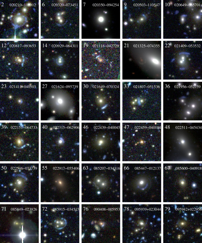
Figure 3.— The SARCS sample showing the 54 promising lens systems with rank of 3 and above. All color cutouts are made from CFHT imaging in $g,r$ and $i$ bands. The cutouts are $\sim$30″on the side. The candidate SA78 is known as COSMOS 5939+3044.

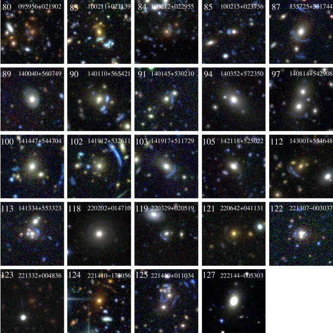
Figure 4.— Continue Fig. 3. The candidates SA83 and SA102 are known as COSMOS 0211+1139 and RCS 1419.2+5326, respectively.

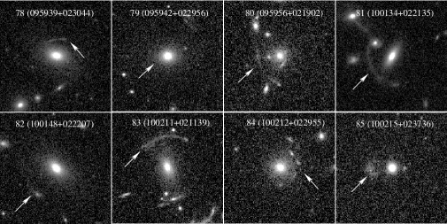
Figure 5.— HST $I$-band (F814W) imaging of the SARCS lens candidates within the D2 field extracted from the COSMOS archive. The IDs and co-ordinates are labelled for each system. The arrows point towards the putative lensed arcs. The arc in SA79 is too faint to be visible in the $I$-band HST image shown here. All candidates are new detections except SA78 (COSMOS ID - 5939+3044) and SA83 (COSMOS ID - 0211+1139). The images are 6″on the side. North is up and East is left.

Table 3 SARCS candidates with follow-up information from the SL2S collaboration.

RA	DEC	Reference	$z_{l}$, $z_{s}$	Comment
02:09:57.67	$-$03:54:57.08	VM	–, –	V, H
02:13:24.52	$-$07:43:54.82	–	0.72, –	K, V, H
02:14:08.07	$-$05:35:32.39	L09,V11	0.444,	V, H
		VM	1.023$\pm$0.001/1.7$\pm$0.1
02:14:11.24	$-$04:05:02.71	M11,VM	0.609, –	K, V, H
02:16:49.25	$-$07:03:23.80	VM	–, –	V, H
02:18:07.29	$-$05:15:36.16	M11	0.647, –	V, H
02:19:56.42	$-$05:27:59.21	VM	–, –	V, H
02:21:51.18	$-$06:47:32.66	L09,VM	0.618,	V, H
02:25:11.04	$-$04:54:33.54	R11	0.238, 1.199	K, H
02:25:46.13	$-$07:37:38.52	L09	0.511,	G
08:52:07.18	$-$03:43:16.28	VM	–, –	V, H
08:54:46.55	$-$01:21:37.08	L09,L10	0.3530$\pm$0.0005,1.2680$\pm$0.0003	K, V, H
08:58:48.83	$-$02:39:25.79	–	–, –	H
08:59:14.55	$-$03:45:14.85	L09,VM	0.647, –	V, H
09:04:07.97	$-$00:59:52.85	–	–, –	H
10:02:11.22	+02:11:39.46	–	–, –	H
14:08:13.82	+54:29:08.12	L09	0.416, –	S, H
14:14:47.19	+54:47:03.59	–	–, –	H
14:19:12.17	+53:26:11.44	–	–, –	H
14:19:17.25	+51:17:28.63	–	–, –	H
14:30:00.65	+55:46:47.97	T10	0.497$\pm$0.001, 1.435$\pm$0.001	G, H
14:31:39.77	+55:33:22.81	T10	0.669$\pm$0.001, –	G, H
22:03:29.03	+02:05:18.89	–	–, –	H
22:13:06.93	$-$00:30:37.05	L09	–, –	H
22:13:31.85	+00:48:36.14	L09	–, –	H
22:14:18.82	+01:10:33.85	–	–, –	H
22:21:43.74	$-$00:53:02.89	L09	0.334, –	S, H

3. RESULTS AND DISCUSSION

In the following subsections, we describe the main findings from the SARCS sample and constraints on average properties of the lens population using statistical properties of the arcs. Note that many of the lens candidates are not confirmed lenses yet and hence, the results should be taken as indicative. Firstly, based on the photometric redshifts of the lenses, we study the lens redshift distribution. Subsequently, we discuss about the abundance of giant arcs and presence of radial arcs in the sample. Finally, we measure the azimuthal distribution and image separation distribution of the arcs and argue their importance as diagnostics for understanding the matter distribution of the lenses, statistically.

3.1. Lens redshift distribution

Figure 6.— Redshift distributions of the lens galaxies from the SARCS sample. The solid histogram corresponds to lenses from the whole sample whereas the dashed histogram corresponds to lenses with giant arcs only. The respective means of their redshift distributions are $z=0.58\pm 0.22$ and $z=0.64\pm 0.19$ where the uncertainties indicate 68% confidence level.

The lenses producing giant arcs (e.g. length-to-width ratio $\geq 10$) consist of clusters which lie at the high end of the halo mass function. The redshift distribution and abundance of such massive clusters depend on the parameters of a cosmological model. Bartelmann et al. (1998) estimated that most of the lensing clusters giving rise to giant arcs should peak at around $z\sim 0.3-0.4$ for the currently accepted standard cosmological model.

We use the CFHTLS photometric redshift catalogs (Coupon et al., 2009) which are generated from the code le phare (Ilbert et al., 2006) to calculate the SARCS lens redshift distribution. The accuracy on the redshifts of galaxies in the WIDE with magnitudes $i<21.5$ is $\sigma_{\Delta z/(1+z)}~{}\sim~{}0.037$ and with magnitudes $22.5<i<23.5$ is $\sigma_{\Delta z/(1+z)}~{}\sim~{}0.08$. In Fig. 6, we show the redshift distribution for all the lenses in the SARCS sample (solid histogram) and for lenses consisting of giant arcs only (dashed histogram). In the appendix B, we describe how we estimated the mean and 1$\sigma$ uncertainty given the redshift measurement errors (see Table LABEL:tab:all). We find that the mean of the lens redshift distribution for the SARCS sample is $z=0.58\pm 0.22$ and that for the sample of giant arcs is $z=0.64\pm 0.19$. We note that the mean of the giant arcs sample is at a higher redshift compared to the peak expected from Bartelmann et al. (1998) but certainly consistent within 2$\sigma$ confidence interval. For comparison, the RCS sample G03 finds that most of the lenses with giant arcs have redshifts upwards of $\sim 0.6$.

We make a qualitative comparison of the redshift distributions of the lens populations from other surveys in the literature (not shown in the figure). However, we note that these surveys have significantly different selection functions and hence, quantitative conclusions should not be drawn. The distribution of lens sample from CASTLES peaks between 0.3 and 0.4 which is lower than the mean redshift of the SARCS sample. CASTLES has a large enough sample of lenses but is not homogeneously selected. Nevertheless, the peaks are consistent within 2$\sigma$ (assuming an error of 0.05) in spite of the differences in the sample selection. The COSMOS lens sample (Faure et al., 2008), on the other hand, is fairly homogeneous but the sample size of confirmed lenses is relatively small. COSMOS has a bimodal lens redshift distribution with a minimum at $\sim 0.5-0.6$. This is in stark contrast with the redshift distribution of SARCS (see Fig. 6).

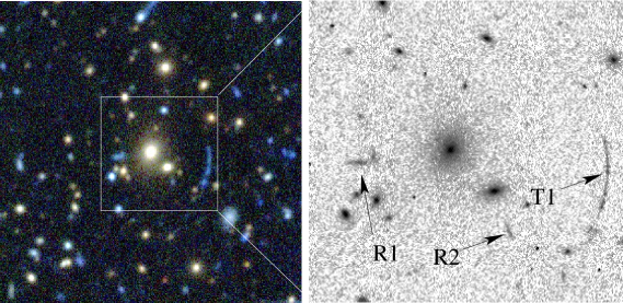
Figure 7.— The CFHTLS $gri$ image of SL2SJ141447+544704 (SA100) on the left and HST F606W ($V$ band) image on the right. The high resolution of HST suggests two radial arc candidates labeled as R1 and R2 whereas the tangential arc labeled as T1 is a confirmed lensed arc. The CFHTLS image is 74.4″on the side and the HST image is $\sim$28.3″on the side.

3.2. Giant and radial arcs

Here, we report detections of giant and radial arcs from our sample. The arcs, both radial and tangential, produced in massive clusters are conventionally referred to as giant arcs, if their length-to-width ($l/w$) ratio is larger than about 8 or 10. For a (non-singular) circularly symmetric projected density profile, the inverse magnification matrix of a lensed image has two eigenvectors, one in the radial and the other in the tangential direction. If the radial eigenvalue becomes 0, then the arcs are magnified and stretched radially with respect to the center of the lens and are called radial arcs. If the tangential eigenvalue becomes 0, then the arcs are magnified and stretched tangentially and are called tangential arcs.

3.2.1 Giant arcs

The statistics of giant arcs allow detection of clusters at the massive end of halo mass function that are rare. The statistics of such rare massive structures is sensitive to the cosmological model of the Universe. Hence, several attempts have been made to predict the giant arcs statistics (e.g., Bartelmann et al., 1998; Wambsganss et al., 2004; Dalal et al., 2004, henceforth, D04) that suggested a large discrepancy compared to the observed abundance of arcs from a well-defined cluster population (e.g., Luppino et al., 1999; Gonzalez et al., 2001; Gladders et al., 2003; Li et al., 2005, 2006). However, the discrepancy has been substantially diminished due to more realistic assumptions such as using a realistic source redshift distribution and improved predictions which consider the contribution of central galaxy or substructure within the halos (e.g., Meneghetti et al., 2000, 2003; Horesh et al., 2005).

We present the abundance of giant arcs in our sample which could be tested with predictions from realistic simulations by taking into account the observational limitations. Within a total unmasked area of $\sim$150 deg², 8 of the arcs have $l/w$ of $\sim$10 or above. Additionally, 4 more arcs have $l/w~{}\sim~{}8$ which are included in the sample of giant arcs because these appear to be broken either due to noise or due to a satellite galaxy. Since one of the giant arcs is from the DEEP, we use rest of the 11 giant arcs from the WIDE data for comparison with RCS. We use the primary sample of RCS which has roughly similar depth compared to WIDE data. The primary RCS lens sample has 6 arcs with $l/w\geq 8$ found within a total area of 90 deg² G03. Therefore, the RCS sample has $0.07\pm 0.03$ arcs deg^-2 which is consistent with the $0.07\pm 0.02$ arcs deg^-2 from the SARCS sample.

3.2.2 Radial arcs

The radial arcs are formed when the source falls on the radial caustic (see Appendix A). The size of the radial caustic and hence, the cross-section to form radial arcs depends on the slope of inner regions of the density profile of the lens (e.g., Hattori et al., 1999). The statistics of radial arcs can thus, be used to constrain the slope of the central density profiles of clusters and thereby, allow a better understanding of the nature of dark matter (Molikawa & Hattori, 2001). More thorough investigations have been carried out to test the effects of realistic assumptions of properties such as lens ellipticity, source size and ellipticity on the statistics of radial and tangential arcs (e.g., Keeton, 2001; Oguri, 2002). Sand et al. (2005) used archival HST (WFPC2) data on various lensing cluster samples to do a systematic study of the number ratio of radial to tangential arc statistics. They accounted for the effects due to the central galaxy in the expected number ratio and placed loose constraints on the slope of the average inner density profile of the dark matter. They underlined the need of larger observational datasets to further explore effects of substructure, mass of the central galaxy and homogeneity of the sample.

We report detections of radial arc candidates in the SARCS sample during the visual inspection. We found 1 candidate which appears like a radial arc in the system SL2SJ141447+544704 (SA100 in Table LABEL:tab:all). This lens system also has a giant tangential arc (T1) with the same color as the radial arc (R1, see the left panel of Fig. 7). The subsequent HST observation in the F606W band shows another radial arc candidate (R2, see right panel of Fig. 7). The nature of the radial arc candidates needs to be verified with spectroscopy and mass modeling since these could be blue edge-on disk galaxies. Radial arcs are usually faint and are overshadowed by the bright central galaxies near which they are formed. Nevertheless, we argue that a follow-up imaging of the promising SARCS candidates at high resolution will help in creating a homogeneous sample of radial and tangential arcs which could provide crucial insights in understanding the density distributions in the inner regions of the lens systems.

3.3. Galaxy-arcs orientation

In this section, we quantify the angular distribution of arcs with respect to the major axis of the ellipticity of the lensing halo. D04 suggested that triaxial dark matter halos, when acting as lenses, usually form lip caustics (e.g., Hattori et al., 1999) and the formation of giant arcs tends to be at the ends of the lip caustics. Using numerical simulations, they showed that the giant arcs are oriented very close to the major axis of the dark matter halo. If a central galaxy is further added to the halo, then it appeared to isotropize the angular distribution of arcs to a small extent. In order to compare these predictions to the observations, D04 measured the angular distribution of giant arcs from the EMSS cluster sample under the assumption that the ellipticity of the lensing galaxy is a good representation of the ellipticity of the underlying DM halo. They found that most of the giant arcs had an orientation of $<$ 45 deg consistent with their predictions.

We use the same definition as that used in D04 for the orientation of the arcs, that is, the angle between the major axis of the lens galaxy and the line connecting the center of the lens galaxy to the midpoint of the arc. The measurement of orientation of real arcs tends to be somewhat subjective since there exists an ambiguity in defining the extent of the arc which is required to find the midpoint of the arc. The midpoint of the arc and its orientation from the major axis of the lens is calculated manually. When there is a single dominant lensing galaxy we measure the position angle (PA) of the major axis of the lens galaxy with sextractor (Bertin & Arnouts, 1996) otherwise we adopt the following strategy. If there are two or three (nearly collinear) lens galaxies with similar colors and brightness, then the PA of the ellipticity is assumed to be along the line joining the lens galaxies. If a circle going through the arc encloses multiple lens galaxies with comparable brightness but no obvious elongation, then such system is rejected. If one of the lens galaxies is predominantly brighter than the companion galaxies, then the ellipticity of the dominant galaxy is assumed to reflect the overall ellipticity of the gravitational potential and hence, of the caustics.

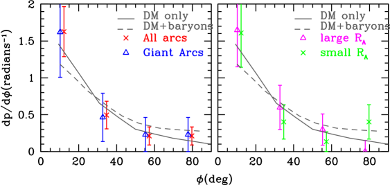
Figure 8.— Angular distribution of arcs with respect to the lens galaxy. The data points in both the panels are from the SARCS sample. In the right panel, the “all arcs” sample is divided into small and large $R_{\rm A}$. The expected curves for dark matter (DM) only (solid) and DM+$3\times 10^{12}h^{-1}M_{\odot}$ (dashed) are taken from D04 which are calculated from the cluster sample of GIF simulation (Kauffmann et al., 1999).

After applying the above selection cuts, we are left with 36 all arc candidates and 11 giant arcs with an average ranking $>2.5$. The angular distribution of the giant arcs from the SARCS sample is shown in the left panel of Fig. 8. We compare the observed distribution to the expected distributions from D04 which correspond to two cases: a) for dark matter only lensing halo (solid curve) and b) a dark matter halo to which a galaxy of $3\times 10^{12}h^{-1}M_{\odot}$ is added (dashed curve). The distribution of giant arcs from our sample appears to follow the expected trend although it is not possible to distinguish between the two cases. We also show the distribution of orientation of all arc candidates (see left panel of Fig. 8) which seems to follow the expected anisotropy. This extends the result obtained by D04 to groups-scale lens systems. Furthermore, we split the all arcs sample into a small $R_{\rm A}$ ($<5\arcsec$) and large $R_{\rm A}$ ($>=5\arcsec$) samples to see the dependence of the angular distribution on the Einstein radius (or the arc radius). The choice of cut at 5″is arbitrary. The baryonic matter tends to make the matter distribution in halos more spherical at the center. Therefore, the angular distribution of arcs for the sample with smaller $R_{\rm A}$ is expected to be more isotropic compared to the sample with large $R_{\rm A}$. However, we do not find any clear differences in the angular distribution of small and large $R_{\rm A}$ for the SARCS sample within the uncertainties (see the right panel of Fig. 8). We note that these measurements may have some systematic errors due to the orientation dependence of the selection function. Ambiguities also exist in the definition of the orientation in few cases, especially when multiple candidate lens galaxies are involved. In addition, the current analysis consists of lens candidates as opposed to confirmed lens systems. Therefore, our conclusions should be treated more of a qualitative nature.

3.4. Image separation distribution

The image separation distribution (ISD) is sensitive to the halo mass, abundance of the lens population, the mass distribution in the lens and the source redshift. Therefore, the ISD measured from galaxy to cluster scales contains information about the cosmological parameters and various scaling relations between galaxy properties and halo mass. Hitherto, the ISD has been measured either at small image separations ($\theta$) primarily, with lens samples such as CASTLES (e.g., Keeton et al., 2000; Khare, 2001) and CLASS (e.g., Kochanek & White, 2001; Oguri, 2006) or at large $\theta$ with cluster-scale lenses, for example, the MACS sample (Zitrin et al., 2011). With the SARCS sample, we can probe the intermediate mass regime corresponding to group scale lenses. The SARCS sample is selected based on the presence of elongated arc-like features and is not directly biased towards selecting a specific lens population. The ISD measured from the lens samples is referred to as the observed ISD and the ISD calculated from various models is referred to as the expected/predicted ISD throughout this paper.

3.4.1 Model for the expected distribution

In the past, the expected ISD was computed with models consisting of either galaxy dominated (e.g., Turner et al., 1984) or dark matter dominated lensing halos (e.g., Narayan & White, 1988). However, since the density profile of dark matter is known to be affected due to the presence of baryons at the center, the need for a more complex model to explain the observed ISD was pointed out by Keeton et al. (1998) and demonstrated by subsequent studies (e.g., Porciani & Madau, 2000; Kochanek & White, 2001; Oguri, 2006, henceforth, O06). We follow the framework developed in O06 and Oguri et al. (2002) to calculate the expected ISD in order to compare it with the observed ISD from the SARCS sample. We also adopt the cosmology used in O06 which constitutes of the following cosmological parameters: $\Omega_{m}=0.3$, $\Omega_{\Lambda}=0.7$ and $\sigma_{8}=0.9$. We describe in detail how each of the model parameters are calculated before proceeding to the comparison of various models.

The probability for a source at redshift, $z_{s}$ to get lensed with image separation greater than $\theta$ is given by

$$P(>\theta;z_{s}) = \int_{0}^{z_{s}}{\rm d}z_{l}\frac{{\rm d}\chi}{{\rm d}z_{l}}\int_{0}^{\infty}{\rm d}M\,n(M,z_{l})$$ (4)

$$\times \sigma_{{\rm lens}}\,\Theta(M-\tilde{M})\,,$$

where $\chi$ is the comoving distance and $z_{l}$ is the redshift of the lens, $M$ corresponds to the halo mass, $n(M,z_{l})$ is the halo mass function, $\tilde{M}$ is the minimum halo mass that causes an image separation equal to $\theta$, and $\Theta$ is the Heaviside step function. The biased lensing cross section, $\sigma_{\rm lens}$ is measured in comoving units and is given by

$$\sigma_{\rm lens}=\pi y_{r}^{2}\xi_{0}^{2}B(z_{s})\,,$$ (5)

where $y_{r}\xi_{0}$ corresponds to the radius of the outermost caustic in the lens plane and it depends on the matter density distribution around the lens. The quantity $B(z_{s})$ denotes the magnification bias which causes sources, fainter than the limiting magnitude of the survey, to be detected in the sample. It is the ratio of the number of sources that can be potentially lensed into an image with luminosity $L$ to the number of sources that have an intrinsic luminosity $L$. In general, the magnification bias depends upon the luminosity of the source and under the assumption of spherical symmetry, it is given by

$$B(z_{s},L)=\frac{1}{\pi y_{r}^{2}\,\Phi(z_{s},L)\,{\rm d}L}\int_{0}^{y_{r}}dy\,2\pi y\,\Phi\Big{(}z_{s},\frac{L}{\mu(y)}\Big{)}\frac{{\rm d}L}{\mu(y)}\,,$$ (6)

where $\Phi(z_{s},L)$ is the true source luminosity function and $\mu(y)$ is the lensing magnification at an angular position $y$ inside the caustic. Under the assumption of a power-law luminosity function which does not evolve with redshift, the luminosity dependence of the magnification bias drops out.

Differentiating both sides of Eq. 4, we obtain the differential probability

$$\bigg{|}\frac{{\rm d}P}{{\rm d}\theta}\bigg{|}=\int_{0}^{z_{s}}{\rm d}z_{l}\frac{{\rm d}\chi}{{\rm d}z_{l}}\int_{0}^{\infty}\frac{{\rm d}M}{{\rm d}\theta}\,n(M,z_{l})\,\sigma_{{\rm lens}}\,\delta[M-\tilde{M}(\theta)]$$

$$=\int_{0}^{z_{s}}{\rm d}z_{l}\,\frac{{\rm d}\chi}{{\rm d}z_{l}}\,n(\tilde{M}[\theta],z_{l})\,\sigma_{{\rm lens}}\frac{{\rm d}\tilde{M}}{{\rm d}\theta}\,,$$ (7)

which can be directly related to the ISD of the observed lens sample.

In O06, the above equation is used to predict the ISD resulting from different components in a given halo. To use the above equation, we have to specify the distribution of mass inside a halo and the halo mass function. The former allows us to calculate $\tilde{M}(\theta)$ and the biased cross section for lensing. For the latter, O06 assumed the then state-of-the-art calibration of the mass function given by Sheth & Tormen (1999). For the mass distribution inside a halo, O06 considered the following different components.

• At the center of the dark matter halo, the matter density is dominated by the central galaxy and the total matter distribution is very close to that of a singular isothermal sphere (SIS). This distribution is given in terms of the one-dimensional velocity dispersion ($\sigma_{\rm vel}$) such that $\rho(r)~{}\propto~{}\sigma^{2}_{\rm vel}/r^{2}$. Following Sect 2.3.1 of Oguri et al. (2002), we calculate the size of the radial caustic ($y_{r}\xi_{0}$) in comoving coordinates, the total magnification of the lensed images and the relation between the velocity dispersion and the image separation for the SIS mass distribution. To relate the mass of the halo to the velocity dispersion of the central galaxy, O06 used galaxy scaling relations. They adopted the halo mass-luminosity relation from Vale & Ostriker (2004) using the abundance matching technique and the Faber-Jackson relation obtained by Bernardi et al. (2003) using SDSS galaxies to relate the luminosity to the velocity dispersion of the galaxy. Following Cooray & Milosavljević (2005), they also included a log-normal scatter in the halo mass-luminosity relation with a scatter of 0.25 dex (see also More et al., 2009b, 2011b).

• On large scales, the distribution of dark matter follows the Navarro-Frenk-White (NFW, Navarro et al., 1997) profile given by

  $$\rho(r)=\frac{\rho_{s}}{(r/r_{s})(1+r/r_{s})^{2}}\,.$$ (8)

  where the scale radius $r_{s}=R_{\rm vir}/c$, the concentration parameter $c$ is related to the mass $M$ with a considerable scatter. O06 used the mean relation between concentration and mass of Bullock et al. (2001), given by

  $$\bar{c}=\frac{10}{1+z}\left(\frac{M}{M_{*}}\right)^{-0.13}\,.$$ (9)

  The distribution of concentrations at fixed halo mass is assumed to be log-normal with a scatter of $0.3$ dex. For the NFW case, we calculate the caustic size, the magnification and the relation between halo mass and the image separation numerically. We defer the details of our procedure to calculate these quantities to the appendix A.

  

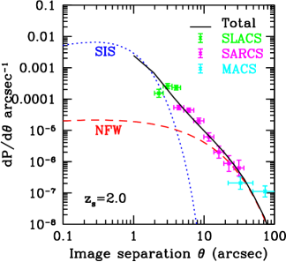
  Figure 9.— Image separation distribution. Theoretically calculated image separation distribution curves for SIS profile (dotted), NFW profile (dashed) and total profile (solid) following the O06 model. The data points from the SLACS (green), SARCS sample (magenta) and MACS (cyan) where the vertical bars indicate Poissonian errors and horizontal bars show the bin width. As discussed in Sect. 3.4.2, we multiply the ISDs of the lens samples by their respective $P(>\theta_{\rm cut})$.

• In addition to the above two simple profiles, O06 also considered a combined total profile which included the central galaxy, the dark matter halo and the effect of adiabatic contraction (AC) of dark matter in response to the baryonic component of the galaxy at the center. In this case, O06 assumed the central galaxy to have a Hernquist profile (Hernquist, 1990), given by

  $$\rho(r)=\frac{M_{b}}{2\pi}\frac{1}{(r/r_{b})(r_{b}+r)^{3}}\,.$$ (10)

  where $M_{b}$ is the stellar mass of the galaxy and $r_{b}$ is a core radius. The stellar mass $M_{b}$ was obtained using the halo mass-luminosity relation found by Vale & Ostriker (2004) and adopting a constant mass-to-light ratio of $3.0h_{70}M_{\odot}/L_{\odot}$. The scaling relations of Bernardi et al. (2003) can be used to obtain the effective radius $R_{0}$ as a function of the luminosity of the galaxy which is related to the core radius of the Hernquist profile such that $r_{b}=0.551R_{0}$. The AC is carried out using the analytical formalism presented by Gnedin et al. (2004). Having specified the total dark matter distribution, the caustic size, the magnification and the relation between halo mass and the image separation need to be calculated numerically. We describe the procedure we use, in the appendix A.

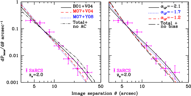
Figure 10.— Image separation distribution. Theoretical curves for the total profile, shown with solid black line, are the same as in Fig. 9. Left: Adopting the $c$-$M$ relation of M07 (dashed) steepens the total profile. The dotted curve, with $M$-$L$ relation of Y08 and $c$-$M$ relation of M07, steepens further but negligibly. The total profile without the AC (dashed-dotted) is also shown. Right: The effect of varying $\alpha_{\rm LF}$ on the ISD is shown for the total profile. The total profile without any bias (long dashed) is independent of $\alpha_{\rm LF}$. Changes in various model parameters have degenerate effects on the expected ISD. The current uncertainties on the data do not have further constraining power on the tested model parameters. All the theoretical curves are multiplied by the P($>\theta_{\rm 3.7\arcsec}$) since the SARCS sample consists of lenses with $\theta>3.7\arcsec$.

O06 assumed the background source population to lie at a redshift of $z_{s}=2$, and the source luminosity function, $\Phi(z_{s},L)\propto L^{-2.1}$ appropriate for the radio survey CLASS (Myers et al., 2003; Rusin & Tegmark, 2001) . We are able to reproduce the expected ISDs from O06, given by Eq. 3.4.1, for all the three density distributions mentioned above. The expected ISDs corresponding to these three density distributions are shown in Fig. 9.

3.4.2 Observed distribution

The observed ISD is calculated by logarithmically binning the image separations of 125 SARCS candidates with $\theta_{\rm cut}\geq 20$ pixels (that is, $>3.7\arcsec$) and an average ranking of 2 and above. The image separation for each lens candidate is taken as twice the Einstein radius or roughly the arc radius which is the distance between the candidate lensed image and the center of respective lens galaxy. Let $\theta-d\theta=\theta_{\rm l}$ and $\theta+d\theta=\theta_{\rm h}$, then the observed ISD is given by

$$\bigg{|}\frac{dP_{\rm lens}}{d\theta}\bigg{|}_{\rm obs}=\frac{P(>\theta_{\rm h})-P(>\theta_{\rm l})}{2d\theta}$$

$$=\frac{N(>\theta_{\rm h})-N(>\theta_{\rm l})}{N(>\theta_{\rm cut})2d\theta}\,.$$ (11)

where the total number of observed lenses is $N(>\theta_{\rm cut})$. While comparing their theoretical predictions ($dP/d\theta$) to the observed ISDs from the CLASS sample, O06 assumed an arbitrary normalization for their data points. Instead we note that,

$$P_{\rm lens}(>\theta) = \frac{N_{\rm lens}(>\theta)}{N_{\rm lens}(>\theta_{\rm cut})}$$ (12)

$$= \frac{N_{\rm lens}(>\theta)}{N_{\rm src}}\frac{N_{\rm src}}{N_{\rm lens}(>\theta_{\rm cut})}\,,$$

$$= \frac{P(>\theta)}{P(>\theta_{\rm cut})}\,,$$

$$\implies\bigg{|}\frac{dP}{d\theta}\bigg{|} = \bigg{|}\frac{dP_{\rm lens}}{d\theta}\bigg{|}\,P(>\theta_{\rm cut})\,.$$ (13)

To facilitate a direct comparison of the observed ISD to the theoretical expectation from O06 (see Eq. 3.4.1), we multiply Eq. 11 by $P(>\theta_{\rm cut})$. The quantity $P(>\theta_{\rm cut})$ is obtained by integrating Eq. 3.4.1 from $\theta_{\rm cut}$ to $\infty$. The SARCS data points are shown in magenta in Fig. 9. The vertical error-bars are calculated assuming Poisson number statistics and the horizontal bars show the bin width.

The SARCS data points demonstrate that the average density profile of the halos, giving rise to the intermediate $\theta$ values ($\sim 3\arcsec-12\arcsec$), is best represented by a combined profile for the main galaxy and the dark matter halo as opposed to a pure SIS or pure NFW profile. It is clear from the Fig. 9 that the SARCS sample follows a steeper ISD at the intermediate scales compared to halos with NFW profile and shallower than halos with only SIS profile.

It is interesting to compare the SARCS sample with the SLACS and MACS samples which span the lower end and higher end of the ISD, respectively. These samples also have different selection functions compared to the SARCS sample. We apply the same procedure to calculate the observed ISD for SLACS and MACS data points shown in Fig. 9. Intriguingly, the SLACS data points lie in the regime where the SIS density profile just ceases to be dominant. Although the SLACS sample appears to be incomplete by a factor of 2 to 3 in the lowest $\theta$ bin, the ISD of SLACS could be seen as an extrapolation of the ISD from the SARCS sample. As expected, the MACS sample is nearly consistent with either the NFW or total profile. Assuming that incompleteness is the only major factor in the ISD of SLACS, the expected ISD corresponding to the total profile best matches the SLACS, SARCS and MACS samples combined.

We note that we have not accounted for any effects due to purity or incompleteness of the SARCS sample in this paper. We suspect that the completeness of the sample as a function of the image separation is not severely affected due to the selection function. We are currently investigating this issue and the results will be presented in a forthcoming paper.

3.4.3 Tests with varying models

Here, we test the effects of varying the different components of the O06 model and compare against the observed ISD. Since different models have different values of $P(>\theta_{\rm cut})$, we predict $dP_{\rm lens}/d\theta$ from each model and compare it with the observed ISD in Fig. 10. We test only for image separations spanning the observed $\theta$ values. In the Fig. 9 and both the panels of Fig. 10, the solid line represents the same ISD corresponding to the total two-component profile which accounts for the contraction of the dark matter. First, we test the influence of excluding the AC while computing the total profile. This has the effect of making the expected ISD shallower as shown by the dashed-dotted curve in the left panel of Fig. 10. Prima facie, the AC model fits the data better than the model without AC. However, as we show below, there are other degeneracies in the model which prevent us from ruling out the “no AC” model at high significance.

Next, we test the effect of using different $c$-$M$ relations on the ISD. For example, we use the $c$-$M$ relation by Macciò et al. (2007, henceforth, M07) instead of that given by Bullock et al. (2001). The $c$-$M$ relation of M07 is roughly 15-20% lower than that of Bullock et al. (2001). The combined profile using the $c$-$M$ relation of M07 is shown by the dashed curve in the left panel of Fig. 10. Within the current statistical limits on the data, both the $c$-$M$ relations appear plausible, although the data appears to slightly favor the $c$-$M$ relation of M07. Since the $c$-$M$ relations differ significantly at small and large image separations, we will need additional samples of galaxy or cluster-scale lenses to test between the different $c$-$M$ relations.

We also test the effect of using a more recent determination of the $M$-$L$ relation obtained by Yang et al. (2008, henceforth, Y08) from a sample of SDSS groups along with the $c$-$M$ relation of M07 for the combined total profile. The $M$-$L$ relation of Y08 differ by $\sim$0.2 dex from that of Vale & Ostriker (2004) at the intermediate mass regime which is the regime of interest. This appears to cause a very negligible change in the predicted ISD.

We try to quantify the effect of varying the slope of the source luminosity function at the faint-end. We show the effect on the combined profile of O06 and vary the power law index, $\alpha_{\rm LF}$ of the source luminosity function, $\Phi(z_{s},L)\propto L^{\alpha_{\rm LF}}$. This influences the lens cross-section via the magnification bias. The solid curve in Fig. 10 shows the expected ISD using the fiducial value of $\alpha_{\rm LF}=-2.1$, while the dotted and short dashed curves show the ISD in the right panel, corresponding to $\alpha_{\rm LF}$ equal to -1.7 and -1.2, respectively. It is evident from the figure that the observed ISD can be used to constrain the slope of the luminosity function, if the statistical error bars could be reduced.

We note that the magnification bias factor in the biased lens cross-section is calculated assuming that the background sources are point sources such as quasars. However, the background sources corresponding to the lensed arcs are mostly galaxies with extended surface brightness and their magnification bias could be negligible (e.g., Narayan & Wallington, 1993). Therefore, we calculate the ISD assuming no bias, that is, by substituting $B(z_{\rm s})=1$ in Eq. 5. The long dashed curve in the right panel of Fig. 10 shows the ISD without the bias.

The data is consistent with all of the above tested models within the uncertainties. The various scaling relations from our model, that are tested here, have degenerate effects on the expected ISD. For example, varying the $c$-$M$ relation has the same effect as changing the slope of the luminosity function or excluding AC. However, constraints from independent observations such as dynamics and strong lensing could be used to determine the $c$-$M$ relation. This will allow us to better constrain the slope of the luminosity function or make more robust statements about AC.

For all the theoretical calculations, we have assumed $z=2$ for the source redshift. We checked the effect of adopting different source redshifts, $z_{s}=1.5$ and $z_{s}=3.0$ on the predicted ISD. We found that using a higher (lower) source redshift causes the predicted ${\rm d}P/{\rm d}\theta$ to be larger (smaller) by roughly a constant factor at all values of $\theta$. However, the predicted ${\rm d}P_{\rm lens}/{\rm d}\theta$ is not affected because the corresponding increase (decrease) in $P(>\theta_{\rm cut})$ almost perfectly cancels out the increase (decrease) in ${\rm d}P/{\rm d}\theta$. This implies that the expected ISD would not be drastically different had we accounted for the distribution of source redshifts instead of assuming a single value for the source redshift.

4. SUMMARY

We have presented the SARCS sample from the completed CFHTLS-WIDE and CFHTLS-DEEP covering a combined unmasked area of $\sim$150 deg² in the sky. The lens sample is compiled through a semi-automatic technique consisting of using arcfinder algorithm, followed by visual inspection and ranking of the candidates. We briefly described the working of the arcfinder (Alard, 2006) and the modifications implemented in the newer version of the algorithm. Although the arcfinder V2.0 is faster, there is still scope for improving the algorithm in terms of increasing the purity without compromising the completeness of the arc detections.

We have compiled a total of 127 candidates in the SARCS sample, out of which 38 are found serendipitously. From the complete sample, 54 are promising lens systems (ranking of 3 and above). A total of 31 systems are almost certain or confirmed systems, out of which 27 systems have been followed-up via techniques such as spectroscopy, high-resolution imaging and/or lens mass modeling. We found 2 radial arc candidates in the SARCS sample and both of them are located in the system SA100. The second radial arc is clearly identified from the high resolution HST imaging only. Our sample may have more radial arcs which could be discovered with high resolution imaging. With statistics of radial and tangential arcs from a homogeneous and a larger sample of lenses, interesting constraints could be placed on the slope of inner density profiles of the dark matter distribution.

We have discovered a total of 12 giant arcs ($l/w\geq 8$) in our sample. Statistics with giant arcs is considered to be a good probe of cluster properties or cosmological parameters but not an easy one. We have presented the redshift distributions of the lens galaxies with giant arcs and all arcs in the SARCS sample using the photometric redshifts and found to have mean values at $z\sim 0.6$. This is somewhat higher than the expected peak at redshift of $0.3-0.4$ (Bartelmann et al., 1998) but consistent within the uncertainties. Note that the predictions need to be revised with improved simulations and more realistic assumptions. We also calculated the angular distribution of giant arcs which are sensitive to the ellipticity of the halo. We found an anisotropy in the orientation of arcs in our sample consistent with that seen in simulated lens clusters (e.g. see D04). In addition, the angular distribution of all arcs from the SARCS sample exhibits similar anisotropy. This anisotropy appears to hold at all arc radii within the current uncertainties albeit needs to be verified with a sample of confirmed lenses. Thus, we have extended this result to group scale halos, observationally. It would be interesting to check if lensed arcs in simulated group scale halos also show a similar anisotropy in their azimuthal distribution and what constraints could be placed on the baryonic physics important in the inner few Kpcs which is probed by these lensed arcs.

We followed the formalism of O06 to calculate the expected ISD in order to compare it with the observed ISD from SARCS sample. We first reproduced the results of O06 and then introduced variations in different scaling relations used in their model. The SARCS sample allowed, for the first time, to probe the intermediate mass regime corresponding to group-scale halos via the ISD. We showed that the density profile of the halos are well-reproduced by a combined profile (NFW and Hernquist) at the group-scales, which is consistent with the predictions. Given the uncertainties in the data and the degeneracies in the model, both the models that account for or exclude the role of AC are consistent with the observed ISD. With the availability of larger statistics of confirmed lenses and understanding of the sample selection function, the distinction between models with and without AC would be possible.

Next, we varied the $c$-$M$ relation, the halo mass-luminosity relation, the slope of a power-law source luminosity function and the source redshift. We found that given the current uncertainties in the observed ISD, the $c$-$M$ relations of both Bullock et al. (2001) and the more recent, Macciò et al. (2007), are plausible. The expected ISD does not vary significantly and fits the data well, if the halo mass-luminosity relations have an uncertainty of $\sim 0.2$ dex. Following O06, we adopted a power-law index of $\alpha_{\rm LF}=-2.1$ for the background source luminosity function to account for the magnification bias. We further tested the effect of varying the $\alpha_{\rm LF}$ on the expected ISD and found to be consistent with the data. However, within the uncertainties, the data is also consistent, if no magnification bias is assumed. We did not test the effects of any evolution of the luminosity function or any other functional form such as a broken power law.

We found that varying the model parameters have degenerate effects on the ISD, for instance, changing the $c$-$M$ relation and changing the slope of the luminosity function, $\alpha_{\rm LF}$. Therefore, using priors from independent methods on one of these relations could help in constraining the others via the observed ISD. Since the background sources are assumed to be at a redshift of 2, we tested the effect of varying the source redshift. The expected ISD (${\rm d}P_{\rm lens}/{\rm d}\theta$) is not affected by choosing different redshifts (z${}_{s}=1,2,3$) between the range we tested.

As described above, we have used arcs statistics to probe the average density profiles of group-scale lenses and we have shown the possibility to use arcs statistics in constraining some scaling relations. However, the models assumed in our work are simplistic and will need refinement as the lens samples become larger with upcoming surveys. On the observational side, understanding the selection effects will also become crucial, if the model parameters need to be constrained with high accuracy. We hope to address some of these important issues in future studies.

Appendix A A. NUMERICAL DETERMINATION OF LENSING QUANTITIES

We describe how we numerically determined the relation between the halo mass and the image separation, the size of radial caustic and the position dependent magnification for general spherically symmetric mass distributions. These are used in the calculation of the expected ISD in the two of the models we tested, namely, the NFW and the total (NFW and Hernquist) profiles.

Let the position of the lens in the plane of the sky be the origin of the coordinate system. The lensing equation relates the true angular position, ${\boldsymbol{\beta}}$, of the background source to the observed angular position of its image, ${\boldsymbol{\theta}}$ in the plane of the sky, such that

$${\boldsymbol{\beta}}={\boldsymbol{\theta}}-{\boldsymbol{\alpha}}({\boldsymbol{\theta}})\,,$$ (A1)

where ${\boldsymbol{\alpha}}$ is the scaled deflection angle. In case of a spherically symmetric density distribution for the lens, the deflection angle ${\boldsymbol{\alpha}}$ lies along the same direction as $\theta$, and the lens equation can be written as

$${\boldsymbol{\beta}}={\boldsymbol{\theta}}-\frac{\alpha(\theta)}{\theta}{\boldsymbol{\theta}}\,,$$ (A2)

where the quantities in normal face are the magnitudes of the corresponding vectors in bold face. The relation between the deflection angle $\alpha$ and the magnitude of the image position $\theta$ is given by

$$\alpha(\theta)=\frac{4GM(<D_{l}\theta)}{c^{2}D_{l}\theta}\,,$$ (A3)

where $D_{l}$ is the angular diameter distance to the lens and $M(<D_{l}\theta)$ denotes the projected lens mass within a physical radius of size $\xi=D_{l}\theta$, which can be obtained using the following equation

$$M(<\xi)=2\pi\int_{0}^{\xi}R^{\prime}{\rm d}R^{\prime}\int_{0}^{R_{\rm max}}2\,\rho\left(\sqrt{z^{2}+R^{\prime 2}}\right)dz\,,$$ (A4)

where $R_{\rm max}=\sqrt{R_{\rm vir}^{2}-\xi^{2}}$ and $R_{\rm vir}$ is the virial radius.

Figure 11.— Source position as a function of image position for spherically symmetric lens density distribution. The center of the lens potential is at the origin. RC is the location of the radial caustic and TCC is the location of the tangential critical curve which corresponds to the Einstein radius.

In Fig. 11, we show the generic shape of how $\beta$ and $\theta$ are related to each other for a spherically symmetric mass distribution which has a finite density at the center (non-singular). For large values of $\beta$, $\theta\approx\beta$ corresponding to the weak lensing regime. As the source approaches the lens in projection, i.e as $\beta\rightarrow 0$, the source position $\beta$ corresponds to multiple values of $\theta$ referred to as the strong lensing regime. The first instance of this is when the source is at the radial caustic (labeled as RC in Fig. 11) and here, the numerical derivative of $\beta$ with respect to $\theta$ is zero. When $\beta\approx 0$, $\theta$ corresponds to the Einstein radius ($\theta_{E}$) which is the location of the tangential critical curve (see TCC in Fig. 11). The image separation is approximately equal to $2\theta_{E}$.

The magnification of the lensed image at $\theta$ is given by the determinant of

$$\mu(\theta)=\left|\frac{\partial{\boldsymbol{\beta}}}{\partial{\boldsymbol{\theta}}}\right|^{-1}\,.$$ (A5)

In component notation, the required derivative is given by

$$\frac{\partial\beta_{i}}{\partial\theta_{j}} = \delta_{ij}\left(1-\frac{\alpha}{\theta}\right)-\frac{\partial}{\partial\theta}\left(\frac{\alpha}{\theta}-1\right)\frac{\partial\theta}{\partial\theta_{j}}\theta_{i}$$ (A6)

$$= \delta_{ij}\frac{\beta}{\theta}+\frac{\partial}{\partial\theta}\left(\frac{\beta}{\theta}\right)\frac{\theta_{i}\theta_{j}}{\theta}$$ (A7)

$$= \delta_{ij}\frac{\beta}{\theta}+\left(\frac{\partial\beta}{\partial\theta}-\frac{\beta}{\theta}\right)\frac{\theta_{i}\theta_{j}}{\theta^{2}}\,.$$ (A8)

The inverse of the determinant of the above equation simplifies to

$$\mu(\theta)=\frac{\theta}{\beta}\frac{\partial\theta}{\partial\beta}\,.$$ (A9)

To summarize, given a spherically symmetric density distribution $\rho(r)$, we first obtain the value of $\beta$ for different values of $\theta$ using equations A2-A4. We use cubic splines to approximate the function $\beta(\theta)$. The value of $\beta$ which corresponds to the local extrema of this function gives the angular size of the radial caustic. The image separation is given by two times the value of $\theta$ when $\beta=0$. The mass within this angular image separation can be calculated using Equation A4. Finally, the magnification as a function of $\theta$ can be obtained using Equation A9. The required derivative is calculated by using the cubic spline fit. The magnification bias can thus be calculated using Equation 6.

Appendix B B. MEASUREMENT OF THE PEAK OF THE REDSHIFT DISTRIBUTION

Consider a lensing galaxy with true redshift $z_{t}$ for which the photometric redshift estimate is $z_{i}\pm\sigma_{i}$. Let us assume that the true redshifts of the lens population follow a Gaussian distribution, $G(\bar{z}_{t},\sigma_{t}^{2})$, with the mean and variance given by $\bar{z}_{t}$ and $\sigma_{t}^{2}$, respectively. The probability that the estimated redshift of the lens galaxy is equal to $z_{i}$, is then given by

$$P(z_{i}|G) = \int P(z_{i}|z_{t})P(z_{t}|G)dz_{t}\,,$$ (B1)

$$= \frac{1}{2\pi}\int\frac{1}{\sigma_{i}\sigma_{t}}{\rm exp}\left[-\left(\frac{(z_{i}-z_{t})^{2}}{2\sigma_{i}^{2}}+\frac{(z_{t}-\bar{z}_{t})^{2}}{2\sigma_{t}^{2}}\right)\right]dz_{t}\,.$$ (B2)

Rewriting the factor inside the exponential as a quadratic in $z_{t}$ and completing the square yields

$$P(z_{i}|G)=\frac{1}{2\pi\sigma_{i}\sigma_{t}}{\rm exp}\left[\frac{-(z_{i}-\bar{z}_{t})^{2}}{2(\sigma_{i}^{2}+\sigma_{t}^{2})}\right]\int{\rm exp}\left[\frac{-\big{[}z_{t}-\tilde{z}\big{]}^{2}}{2}\left(\frac{1}{\sigma_{i}^{2}}+\frac{1}{\sigma_{t}^{2}}\right)\right]dz_{t}\,,$$ (B4)

where $\tilde{z}=(\sigma_{i}^{2}+\sigma_{t}^{2})^{-1}(z_{i}\sigma_{i}^{-2}+{\bar{z}}_{t}\sigma_{t}^{-2})$. Carrying out the integral gives

$$P(z_{i}|G) = \frac{1}{\sqrt{2\pi(\sigma_{i}^{2}+\sigma_{t}^{2})}}{\rm exp}\left[\frac{-(z_{i}-\bar{z}_{t})^{2}}{2(\sigma_{i}^{2}+\sigma_{t}^{2})}\right]\,.$$ (B5)

Since the determinations of the photometric redshifts of lens galaxies are independent of each other, the combined likelihood for the data, given our model, can be written as $\mathscr{L}=\prod_{i=1}^{N}P(z_{i}|G)$. The posterior distribution for our model parameters given the data is then given by Bayes’ theorem

$$P(\bar{z}_{t},\sigma_{t}^{2}|z_{i},\sigma_{i})\propto\mathscr{L}\,P(\bar{z}_{t},\sigma_{t}^{2})$$ (B6)

We assume uninformative priors on the parameters $\bar{z}_{t}$ and $\sigma_{t}^{2}$ and sample from the above posterior distribution using a Monte Carlo Markov Chain. We quote the mean of the redshift distribution and the 68 percent confidence interval on it using the samples from the chain.

References

- Alard & Lupton (1998) Alard, C., & Lupton, R. H. 1998, ApJ, 503, 325
- Alard (2006) Alard, C. 2006, arXiv:astro-ph/0606757
- Auger et al. (2010) Auger, M. W., Treu, T., Bolton, A. S., et al. 2010, ApJ, 724, 511
- Balogh et al. (2009) Balogh, M. L., et al. 2009, MNRAS, 398, 754
- Balogh et al. (2011) Balogh, M. L., et al. 2011, MNRAS, 412, 2303
- Barnabè et al. (2009) Barnabè, M., Czoske, O., Koopmans, L. V. E., et al. 2009, MNRAS, 399, 21
- Bartelmann et al. (1998) Bartelmann, M., Huss, A., Colberg, J. M., Jenkins, A., & Pearce, F. R. 1998, A&A, 330, 1
- Bernardi et al. (2003) Bernardi, M., et al. 2003, AJ, 125, 1866
- Bertin & Arnouts (1996) Bertin, E., & Arnouts, S. 1996, A&AS, 117, 393
- Blandford & Narayan (1986) Blandford, R., & Narayan, R. 1986, ApJ, 310, 568
- Blandford & Narayan (1992) Blandford, R. D., & Narayan, R. 1992, ARA&A, 30, 311
- Bolton et al. (2004) Bolton, A. S., Burles, S., Schlegel, D. J., Eisenstein, D. J., & Brinkmann, J. 2004, AJ, 127, 1860
- Bolton et al. (2006) Bolton, A. S., Burles, S., Koopmans, L. V. E., Treu, T., & Moustakas, L. A. 2006, ApJ, 638, 703
- Bullock et al. (2001) Bullock, J. S., Kolatt, T. S., Sigad, Y., Somerville, R. S., Kravtsov, A. V., Klypin, A. A., Primack, J. R., & Dekel, A. 2001, MNRAS, 321, 559
- Cabanac et al. (2007) Cabanac, R. A., et al. 2007, A&A, 461, 813
- Coles (2008) Coles, J. 2008, ApJ, 679, 17
- Cooray & Milosavljević (2005) Cooray, A., & Milosavljević, M. 2005, ApJ, 627, L89
- Coupon et al. (2009) Coupon, J., et al. 2009, A&A, 500, 981
- Dai et al. (2010) Dai, X., Bregman, J. N., Kochanek, C. S., & Rasia, E. 2010, ApJ, 719, 119
- Dalal et al. (2004) Dalal, N., Holder, G., & Hennawi, J. F. 2004, ApJ, 609, 50
- Ebeling et al. (2001) Ebeling, H., Edge, A. C., & Henry, J. P. 2001, ApJ, 553, 668
- Falco et al. (1999) Falco, E. E., et al. 1999, ApJ, 523, 617
- (23) Fassnacht, C. D., Moustakas, L. A., Casertano, S., et al. 2004, ApJ, 600, L155
- Faure et al. (2008) Faure, C., et al. 2008, ApJS, 176, 19
- (25) Faure, C., Anguita, T., Alloin, D., et al. 2011, A&A, 529, A72
- Feldmann et al. (2006) Feldmann, R., et al. 2006, MNRAS, 372, 565
- Ferreras et al. (2010) Ferreras, I., Saha, P., Leier, D., Courbin, F., & Falco, E. E. 2010, MNRAS, 409, L30
- Gavazzi et al. (2007) Gavazzi, R., Treu, T., Rhodes, J. D., Koopmans, L. V. E., Bolton, A. S., Burles, S., Massey, R. J., & Moustakas, L. A. 2007, ApJ, 667, 176
- Gladders et al. (2003) Gladders, M. D., Hoekstra, H., Yee, H. K. C., Hall, P. B., & Barrientos, L. F. 2003, ApJ, 593, 48
- Gnedin et al. (2004) Gnedin, O. Y., Kravtsov, A. V., Klypin, A. A., & Nagai, D. 2004, ApJ, 616, 16
- Gonzalez et al. (2001) Gonzalez, A. H., Zaritsky, D., Dalcanton, J. J., & Nelson, A. 2001, ApJS, 137, 117
- Grillo et al. (2010) Grillo, C., Eichner, T., Seitz, S., Bender, R., Lombardi, M., Gobat, R., & Bauer, A. 2010, ApJ, 710, 372
- Hattori et al. (1999) Hattori, M., Kneib, J., & Makino, N. 1999, Progress of Theoretical Physics Supplement, 133, 1
- Helsdon & Ponman (2000) Helsdon, S. F., & Ponman, T. J. 2000, MNRAS, 315, 356
- Hernquist (1990) Hernquist, L. 1990, ApJ, 356, 359
- Horesh et al. (2005) Horesh, A., Ofek, E. O., Maoz, D., Bartelmann, M., Meneghetti, M., & Rix, H.-W. 2005, ApJ, 633, 768
- Ilbert et al. (2006) Ilbert, O., et al. 2006, A&A, 457, 841
- Impellizzeri et al. (2008) Impellizzeri, C. M. V., McKean, J. P., Castangia, P., Roy, A. L., Henkel, C., Brunthaler, A., & Wucknitz, O. 2008, Nature, 456, 927
- Jackson (2008) Jackson, N. 2008, MNRAS, 389, 1311
- Jiang & Kochanek (2007) Jiang, G., & Kochanek, C. S. 2007, ApJ, 671, 1568
- Kauffmann et al. (1999) Kauffmann, G., Colberg, J. M., Diaferio, A., & White, S. D. M. 1999, MNRAS, 303, 188
- Keeton et al. (1998) Keeton, C. R., Kochanek, C. S., & Falco, E. E. 1998, ApJ, 509, 561
- Keeton et al. (2000) Keeton, C. R., Christlein, D., & Zabludoff, A. I. 2000, ApJ, 545, 129
- Keeton (2001) Keeton, C. R. 2001, ApJ, 562, 160
- Khare (2001) Khare, P. 2001, ApJ, 550, 153
- Kochanek & White (2001) Kochanek, C. S., & White, M. 2001, ApJ, 559, 531
- Kochanek et al. (2006) Kochanek, C. S., Mochejska, B., Morgan, N. D., & Stanek, K. Z. 2006, ApJ, 637, L73
- Kochanek (2006) Kochanek, C. S. 2006, Saas-Fee Advanced Course 33: Gravitational Lensing: Strong, Weak and Micro,
- Koopmans & Treu (2003) Koopmans, L. V. E., & Treu, T. 2003, ApJ, 583, 606 91
- Koopmans et al. (2006) Koopmans, L. V. E., Treu, T., Bolton, A. S., Burles, S., & Moustakas, L. A. 2006, ApJ, 649, 599
- Koopmans et al. (2009) Koopmans, L. V. E., Bolton, A., Treu, T., et al. 2009, ApJ, 703, L51
- Krusch et al. (2006) Krusch, E., Rosenbaum, D., Dettmar, R.-J., et al. 2006, A&A, 459, 759
- Lenzen et al. (2004) Lenzen, F., Schindler, S., & Scherzer, O. 2004, A&A, 416, 391
- Li et al. (2005) Li, G.-L., Mao, S., Jing, Y. P., et al. 2005, ApJ, 635, 795
- Li et al. (2006) Li, G. L., Mao, S., Jing, Y. P., et al. 2006, MNRAS, 372, L73
- Limousin et al. (2009) Limousin, M., et al. 2009, A&A, 502, 445
- Limousin et al. (2010) Limousin, M., Jullo, E., Richard, J., et al. 2010, A&A, 524, A95
- Lintott et al. (2008) Lintott, C. J., Schawinski, K., Slosar, A., et al. 2008, MNRAS, 389, 1179
- Luppino et al. (1999) Luppino, G. A., Gioia, I. M., Hammer, F., Le Fèvre, O., & Annis, J. A. 1999, A&AS, 136, 117
- Macciò et al. (2007) Macciò, A. V., Dutton, A. A., van den Bosch, F. C., Moore, B., Potter, D., & Stadel, J. 2007, MNRAS, 378, 55
- Mandelbaum et al. (2008) Mandelbaum, R., Seljak, U., & Hirata, C. M. 2008, JCAP, 8, 6
- Marshall et al. (2009) Marshall, P. J., Hogg, D. W., Moustakas, L. A., et al. 2009, ApJ, 694, 924
- (63) Mediavilla, E., et al., 2009, ApJ, 706, 1451
- Meneghetti et al. (2000) Meneghetti, M., Bolzonella, M., Bartelmann, M., Moscardini, L., & Tormen, G. 2000, MNRAS, 314, 338
- Meneghetti et al. (2003) Meneghetti, M., Bartelmann, M., & Moscardini, L. 2003, MNRAS, 346, 67
- Meneghetti et al. (2011) Meneghetti, M., Fedeli, C., Zitrin, A., Bartelmann, M., Broadhurst, T., Gottlöber, S., Moscardini, L., & Yepes, G. 2011, A&A, 530, A17
- Molikawa & Hattori (2001) Molikawa, K., & Hattori, M. 2001, ApJ, 559, 544
- More et al. (2008) More, A., McKean, J. P., Muxlow, T. W. B., Porcas, R. W., Fassnacht, C. D., & Koopmans, L. V. E. 2008, MNRAS, 384, 1701
- More et al. (2009a) More, A., McKean, J. P., More, S., Porcas, R. W., Koopmans, L. V. E., & Garrett, M. A. 2009, MNRAS, 394, 174
- More et al. (2009b) More, S., van den Bosch, F. C., Cacciato, M., et al. 2009, MNRAS, 392, 801
- More et al. (2011a) More, A., Jahnke, K., More, S., Gallazzi, A., Bell, E. F., Barden, M., Häußler, B. 2011, ApJ, 734, 69
- More et al. (2011b) More, S., van den Bosch, F. C., Cacciato, M., et al. 2011, MNRAS, 410, 210
- Muñoz et al. (1998) Muñoz, J. A., Falco, E. E., Kochanek, C. S., Lehár, J., McLeod, B. A., Impey, C. D., Rix, H.-W., & Peng, C. Y. 1998, Ap&SS, 263, 51
- Myers et al. (2003) Myers, S. T., et al. 2003, MNRAS, 341, 1
- Narayan & White (1988) Narayan, R., & White, S. D. M. 1988, MNRAS, 231, 97P
- Narayan & Wallington (1993) Narayan, R., & Wallington, S., 1993, Liege International Astrophysical Colloquia, 31, 217
- Navarro et al. (1997) Navarro, J. F., Frenk, C. S., & White, S. D. M. 1997, ApJ, 490, 493
- Oguri et al. (2002) Oguri, M., Taruya, A., Suto, Y., & Turner, E. L. 2002, ApJ, 568, 488
- Oguri (2002) Oguri, M. 2002, ApJ, 573, 51
- Oguri (2006) Oguri, M. 2006, MNRAS, 367, 1241
- Parker et al. (2005) Parker, L. C., Hudson, M. J., Carlberg, R. G., & Hoekstra, H. 2005, ApJ, 634, 806
- Porciani & Madau (2000) Porciani, C., & Madau, P. 2000, ApJ, 532, 679
- Ratnatunga et al. (1999) Ratnatunga, K. U., Griffiths, R. E., & Ostrander, E. J. 1999, AJ, 117, 2010
- Richard et al. (2011) Richard, J., Kneib, J.-P., Ebeling, H., et al. 2011, MNRAS, 414, L31
- Rines & Diaferio (2010) Rines, K., & Diaferio, A. 2010, AJ, 139, 580
- Ruff et al. (2011) Ruff, A. J., Gavazzi, R., Marshall, P. J., Treu, T., Auger, M. W., & Brault, F. 2011, ApJ, 727, 96
- Rusin & Tegmark (2001) Rusin, D., & Tegmark, M. 2001, ApJ, 553, 709
- Sand et al. (2005) Sand, D. J., Treu, T., Ellis, R. S., & Smith, G. P. 2005, ApJ, 627, 32
- Scoville et al. (2007) Scoville, N., Aussel, H., Brusa, M., et al. 2007, ApJS, 172, 1
- Seidel & Bartelmann (2007) Seidel, G., & Bartelmann, M. 2007, A&A, 472, 341
- Sheth & Tormen (1999) Sheth, R. K., & Tormen, G. 1999, MNRAS, 308, 119
- Sonnenfeld et al. (2011) Sonnenfeld, A., Treu, T., Gavazzi, R., et al. 2011, arXiv:1111.4215
- Suyu & Halkola (2010) Suyu, S. H., & Halkola, A. 2010, A&A, 524, A94
- Suyu et al. (2010) Suyu, S. H., Marshall, P. J., Auger, M. W., Hilbert, S., Blandford, R. D., Koopmans, L. V. E., Fassnacht, C. D., & Treu, T. 2010, ApJ, 711, 201
- Swinbank et al. (2009) Swinbank, A. M., Webb, T. M., Richard, J., et al. 2009, MNRAS, 400, 1121
- Sygnet et al. (2010) Sygnet, J. F., Tu, H., Fort, B., & Gavazzi, R. 2010, A&A, 517, A25
- Thanjavur et al. (2010) Thanjavur, K., Crampton, D., & Willis, J. 2010, ApJ, 714, 1355
- Treu & Koopmans (2002a) Treu, T., & Koopmans, L. V. E. 2002, ApJ, 575, 87
- Treu & Koopmans (2002b) Treu, T., & Koopmans, L. V. E. 2002, MNRAS, 337, L6
- Treu et al. (2010) Treu, T., Auger, M. W., Koopmans, L. V. E., Gavazzi, R., Marshall, P. J., & Bolton, A. S. 2010, ApJ, 709, 1195
- Turner et al. (1984) Turner, E. L., Ostriker, J. P., & Gott, J. R., III 1984, ApJ, 284, 1
- Vale & Ostriker (2004) Vale, A., & Ostriker, J. P. 2004, MNRAS, 353, 189
- Verdugo et al. (2011) Verdugo, T., Motta, V., Muñoz, R. P., Limousin, M., Cabanac, R., & Richard, J. 2011, A&A, 527, A124
- Vegetti et al. (2010a) Vegetti, S., Czoske, O., & Koopmans, L. V. E. 2010, MNRAS, 407, 225
- Vegetti et al. (2010b) Vegetti, S., Koopmans, L. V. E., Bolton, A., Treu, T., & Gavazzi, R. 2010, MNRAS, 408, 1969
- Wambsganss et al. (2004) Wambsganss, J., Bode, P., & Ostriker, J. P. 2004, ApJ, 606, L93
- Warren et al. (1996) Warren, S. J., Hewett, P. C., Lewis, G. F., et al. 1996, MNRAS, 278, 139
- Wyithe (2004) Wyithe, J. S. B. 2004, MNRAS, 351, 1266
- Yang et al. (2008) Yang, X., Mo, H. J., & van den Bosch, F. C. 2008, ApJ, 676, 248
- Zaritsky & Gonzalez (2003) Zaritsky, D., & Gonzalez, A. H. 2003, ApJ, 584, 691
- Zitrin & Broadhurst (2009) Zitrin, A., & Broadhurst, T. 2009, ApJ, 703, L132
- Zitrin et al. (2011) Zitrin, A., Broadhurst, T., Barkana, R., Rephaeli, Y., & Benítez, N. 2011, MNRAS, 410, 1939