Periodic magnetorotational dynamo action as a prototype of
nonlinear magnetic field generation in shear flows

Abstract

The nature of dynamo action in shear flows prone to magnetohydrodynamic instabilities is investigated using the magnetorotational dynamo in Keplerian shear flow as a prototype problem. Using direct numerical simulations and Newton’s method, we compute an exact time-periodic magnetorotational dynamo solution to the three-dimensional dissipative incompressible magnetohydrodynamic equations with rotation and shear. We discuss the physical mechanism behind the cycle and show that it results from a combination of linear and nonlinear interactions between a large-scale axisymmetric toroidal magnetic field and non-axisymmetric perturbations amplified by the magnetorotational instability. We demonstrate that this large-scale dynamo mechanism is overall intrinsically nonlinear and not reducible to the standard mean-field dynamo formalism. Our results therefore provide clear evidence for a generic nonlinear generation mechanism of time-dependent coherent large-scale magnetic fields in shear flows and call for new theoretical dynamo models. These findings may offer important clues to understand the transitional and statistical properties of subcritical magnetorotational turbulence.

I Introduction

The generation of coherent, system-scale magnetic fields in flows of electrically conducting fluids is a long-standing magnetohydrodynamics (MHD) problem which has so far mostly been analyzed in terms of linear, kinematic mean-field dynamo action (Moffatt, 1977). Mean-field effects have in particular long been invoked to explain the origin of magnetic cycles in MHD rotating shear flows (Parker, 1955; Brandenburg and Subramanian, 2005). However, there is currently no mathematical theory and only little physical understanding of mean-field dynamos in parameter regimes (kinetic and magnetic Reynolds numbers) typical of laboratory dynamo experiments and natural MHD shear flows. Overall, the physical nature of dynamo action in such flows remains a mostly open question, with critical implications for geophysics and astrophysics.

Studying the dynamics of shear flows prone to the development of various local three-dimensional (3D) MHD instabilities is one of the most promising avenues of research on this problem. Numerical simulations of this class of flows have explicitly demonstrated their potential for coherent dynamo action (Brandenburg et al., 1995; Hawley et al., 1996; Drecker et al., 2000; Spruit, 2002; Cline et al., 2003; Braithwaite, 2006; Rincon et al., 2007; Lesur and Ogilvie, 2008a; Davis et al., 2010; Tobias et al., 2011), and it has occasionally been pointed out that their dynamics differs markedly from that of kinematic mean-field dynamos, as magnetic field amplification does not proceed exponentially in time and requires finite-amplitude magnetic perturbations coupling dynamically to fluid motions. Identifying the physical mechanisms underlying this behaviour is of prime importance to improve our understanding of dynamo action.

It has recently been realized that these instability-driven (Spruit, 2002; Cline et al., 2003) or subcritical dynamos in shear flows (Rincon et al., 2007, 2008; Rempel et al., 2010) bear many similarities to the hydrodynamic transition to turbulence of shear flows (Hamilton et al., 1995; Waleffe, 1997; Faisst and Eckhardt, 2004; Hof et al., 2006; Eckhardt et al., 2007), a fundamentally nonlinear process whose dynamics involves a variety of hydrodynamic coherent structures such as equilibria, travelling waves (Waleffe, 1998; Faisst and Eckhardt, 2003; Wedin and Kerswell, 2004; Gibson et al., 2009) or limit cycles (Kawahara and Kida, 2001; Toh and Itano, 2003; Viswanath, 2007; Halcrow et al., 2009). This naturally raises the question of the existence and dynamical relevance of coherent structures in MHD shear flows. Most importantly for dynamo theory, could time-dependent large-scale dynamo action in such flows be explained in terms of 3D nonlinear dynamo cycles ? Besides, if nonlinear dynamo cycles exist for this kind of systems, what can be learned from them regarding how turbulence originates and develops in MHD shear flows ?

The problem of magnetorotational (MRI) dynamo action in Keplerian flow (often referred to as “zero net flux MRI”), encountered in the context of astrophysical accretion disks Balbus and Hawley (1998), is particularly interesting to address these questions, as direct numerical simulations display pseudo-cyclic magnetic dynamics (Brandenburg et al., 1995; Lesur and Ogilvie, 2008a; Davis et al., 2010) and indicate that transition to sustained MHD turbulence is intrinsically 3D and nonlinear Hawley et al. (1996). Besides, numerical MRI dynamo turbulence seems to have finite lifetime and to be structured around a chaotic saddle (Rempel et al., 2010), much like hydrodynamic turbulence in pipe flow (Faisst and Eckhardt, 2004; Hof et al., 2006). The search for coherent MRI dynamo structures such as nonlinear cycles is still in its infancy, though. Progress on these matters is not only desirable from a general dynamo perspective, it would also shed light on the transitional properties of MRI turbulence (Fromang et al., 2007) and on its dynamical properties (saturation, transport) in fully developed regimes.

The only exact MRI dynamo structure known as yet is a nonlinear equilibrium in Keplerian MHD plane Couette flow with walls (Rincon et al., 2007), and it only exists for a limited range of parameters. In this work, we report the first accurate calculation of a 3D nonlinear MRI dynamo limit cycle at moderate (transitional) kinetic and magnetic Reynolds numbers using numerical techniques similar to those used for computing nonlinear hydrodynamic cycles in plane Couette flow (Viswanath, 2007). The study of this nonlinear MRI dynamo cycle enables us to investigate in detail the essential physical mechanisms underlying sustained time-dependent MRI dynamo action. In particular, we show that the cycle dynamics is not amenable to a standard mean-field dynamo description, thereby providing clear and detailed evidence for a fully nonlinear mechanism of coherent magnetic field generation in shear flows prone to MHD instabilities.

The paper is organized as follows. In Sect. II, we introduce the theoretical framework and numerical methods used in the study. In Sect. III, we discuss the physical principles of the MRI dynamo and describe our strategy to excite large-scale, coherent recurrent dynamics in direct numerical simulations. Section IV is devoted to the presentation and detailed analysis of the main result of the paper, namely the discovery of a nonlinear MRI dynamo cycle computed thanks to a Newton algorithm. A discussion (Sect. V) of the results and of their possible implications for dynamo theory, astrophysics and research on hydrodynamic shear flows concludes the paper.

II Theoretical and numerical framework

II.1 The shearing sheet

We use the shearing sheet approach to differentially rotating flows (Goldreich and Lynden-Bell, 1965), whereby a cylindrically symmetric differential rotation profile is approximated locally by a linear shear flow $\boldsymbol{U}_{s}=-Sx\,\boldsymbol{e}_{y}$ and a uniform rotation rate $\boldsymbol{\Omega}=\Omega\,\boldsymbol{e}_{z}$. For a Keplerian flow, $\Omega=(2/3)\,S$. Here, $(x,y,z)$ are respectively the shearwise, streamwise and spanwise directions (radial, azimuthal and vertical in accretion disks). The geometry of the shearing sheet is represented in Fig. 1. To comply with dynamo terminology, we refer to the $(x,z)$ projection of vector fields as their poloidal component and to their $y$ projection as their toroidal component. “Axisymmetric” fields have no $y$ dependence. For readers familiar with hydrodynamic plane Couette flow, non-axisymmetric perturbations in our problem correspond to “streamwise-dependent” perturbations in plane Couette flow.

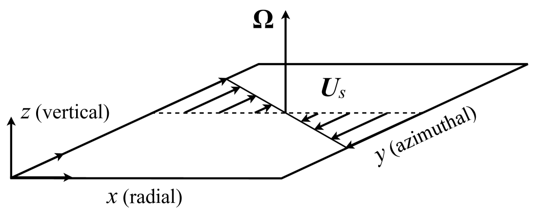
Figure 1: Geometry of the shearing sheet. For a Keplerian flow, the vorticity of $\boldsymbol{U}_{s}$ is anti-aligned with the rotation vector.

We consider incompressible velocity perturbations $\boldsymbol{u}$ and magnetic field $\boldsymbol{B}$ whose evolutions obey the 3D dissipative MHD equations in an unstratified shearing sheet:

$$\frac{\partial\,\boldsymbol{u}}{\partial t}-Sx\,\frac{\partial\,\boldsymbol{u}}{\partial y}+\boldsymbol{u}\cdot\boldsymbol{\nabla}{\,\boldsymbol{u}} = -2\,\Omega\times\boldsymbol{u}+S\,u_{x}\,\boldsymbol{e}_{y}-\boldsymbol{\nabla}{\,\Pi}$$ (1)

$$+\boldsymbol{B}\cdot\boldsymbol{\nabla}{\boldsymbol{B}}+\nu\Delta\,\boldsymbol{u}\,,$$

$$\frac{\partial\boldsymbol{B}}{\partial t}-Sx\,\frac{\partial\boldsymbol{B}}{\partial y}=-SB_{x}\,\boldsymbol{e}_{y}+\boldsymbol{\nabla}\times{\left(\boldsymbol{u}\times\boldsymbol{B}\right)}+\eta\Delta\boldsymbol{B}\,,$$ (2)

$$\boldsymbol{\nabla}\cdot{\boldsymbol{u}}=0\,,\,\,\,\,\boldsymbol{\nabla}\cdot{\boldsymbol{B}}=0\,.$$ (3)

The kinetic and magnetic Reynolds numbers are defined according to $\mathrm{Re}=SL^{2}/\nu$ and $\mathrm{Rm}=SL^{2}/\eta$, where $\nu$ and $\eta$ are the constant kinematic viscosity and magnetic diffusivity and $L$ is a typical scale of the spatial domain considered. $\Pi$ is the total pressure (including magnetic pressure) and $\boldsymbol{B}$ is expressed as an equivalent Alfvén velocity. In the following, velocity and magnetic field amplitudes are measured with respect to $SL$, while times are measured with respect to the inverse of the shearing rate $S^{-1}$.

II.2 Strategy for capturing cycles

Eqs. (1)-(3) are often implemented numerically using the cartesian shearing box model described in Sect. II.3 below. In the regime of Keplerian differential rotation, MRI dynamo action has been found in a large number of independent direct numerical simulations of this kind (Brandenburg et al., 1995; Hawley et al., 1996; Fleming et al., 2000; Fromang et al., 2007; Lesur and Ogilvie, 2008a), sometimes in the form of pseudo-cyclic dynamics. Our strategy to capture a nonlinear MRI dynamo cycle in this regime follows that used in Ref. Viswanath (2007) to compute nonlinear cycles in hydrodynamic plane Couette flow. First, we tried to excite pseudo-cyclic dynamics in direct shearing box numerical simulations (DNS) by devising initial conditions inspired by our partial knowledge of the underlying physics. Once this was achieved, we attempted to converge to a cycle using a Newton solver seeded with a well-chosen DNS snapshot and an estimate for the cycle period. The first part of this program is described in Sect. III. Convergence to a cycle using Newton’s method is presented in Sect. IV. The numerical methods for achieving this result are explained below.

II.3 Numerical method for direct numerical simulations

The numerics presented in this paper are done in the incompressible cartesian shearing box framework, which assumes simple spatial periodicity in the $y$ and $z$ directions and shear-periodicity in the $x$ direction. The latter amounts to assuming that a linear shear flow is constantly imposed and that all quantities are periodic in a sheared Lagragian frame. This approximation is justified in the context of centrifugally supported differentially rotating flows, such as astrophysical accretion flows. Simulations of this kind are also sometimes referred to as homogeneous shear flow turbulence simulations (see e.g. Ref. (Pumir, 1996; Gualtieri et al., 2002)).

Time integrations (direct numerical simulations) are carried out in a shearing box of size $(L_{x},L_{y},L_{z})$ using the SNOOPY code (Lesur and Longaretti, 2007). The numerical time integration scheme used is a standard explicit third-order Runge-Kutta algorithm. The code relies on a spectral implementation of the shearing box model similar to that described in Ref. Umurhan and Regev (2004). A discrete spectral basis of “shearing waves” (or Orr-Kelvin waves, see Refs. Thomson (Lord Kelvin); Orr (1907)) with constant $k_{y}$ and $k_{z}$ wavenumbers and constant shearwise Lagrangian wavenumber $k_{x}^{(0)}$ is used to represent the various fields in the sheared Lagragian frame. The shearing of non-axisymmetric perturbations in this model is described using time-dependent Eulerian shearwise wavenumbers,

$$k_{x}(t)=k_{x}^{(0)}+k_{y}St~{}.$$ (4)

This equation for the radial wavenumber provides an exact description of the evolution of non-axisymmetric waves with initially leading polarization ($k_{x}^{(0)}\,k_{y}<0$) into trailing waves ($k_{x}(t)\,k_{y}>0$, corresponding to a trailing spiral in cylindrical geometry) under the action of shear.

An important comment is in order at this stage. If we were to simply consider the evolution of a given initial set of such waves, we would only be able to observe dynamics that decay on long times. Indeed, the fate of all shearing waves is to evolve into strongly trailing structures with ever smaller scale in $x$, and such structures are extremely efficiently dissipated by viscous and resistive processes (see e.g. Ref. (Knobloch, 1985; Korycansky, 1992)). In order to accomodate for possible physical interactions leading to long-lived nonlinear dynamics in numerical shearing box simulations, a procedure must therefore be used that leaves open the possibility of physical generation and dynamical evolution of new leading non-axisymmetric structures in the course of the simulations. The solution to this problem is to regularly “remap” the basis of shearing waves used to describe the various fields. At regular time intervals during the simulations, the energy content of strongly trailing shearing waves is set to zero, the corresponding basis vector is pruned and replaced by a new shearing wave basis vector with strongly leading wavenumber (see Ref. Lesur (2007), Chap. 5, Sect. 4). If the simulation is well resolved spatially (as is the case for the results presented in this manuscript), the energy contained into strongly trailing waves when they are pruned should be negligible (as a result of their enhanced dissipation), and the remap procedure should not therefore artificially affect the dynamical evolution of the system in any significant way. A way to check this is to compare the energy lost by this procedure with the energy dissipated by viscous/resistive diffusion. We always find that artificial energy losses are negligible in SNOOPY for spatially well-resolved simulations (Lesur and Longaretti, 2005). We also point out that the remap procedure does not by itself inject energy into new leading waves but merely provides room for them in the wavenumber grid. Finally, we emphasize that all nonlinearities of the shearing sheet MHD Eqs. (1)-(3), including nonlinear interactions between all the shearing waves present at a given spatial resolution, are retained in our numerical model. A standard pseudo-spectral method with dealiasing is used to compute all nonlinear terms at each time step.

II.4 Newton’s method for computing nonlinear cycles

Newton’s method is a standard tool for computing nonlinear coherent structures such as saddle points, travelling waves, or nonlinear cycles in high-dimensional dynamical systems. In recent years, the method has been applied successfully to the three-dimensional Navier-Stokes equations for various wall-bounded shear flows (Waleffe, 1998; Faisst and Eckhardt, 2003; Wedin and Kerswell, 2004; Viswanath, 2007; Gibson et al., 2009; Halcrow et al., 2009) and to the MHD equations in Keplerian plane Couette flow Rincon et al. (2007). For the purpose of this study, we developed a new Newton solver called PEANUTS. The solver makes use of the PETSc toolkit (Balay et al., 2011) and is based on an efficient matrix-free Newton-Krylov algorithm particularly well adapted to calculations for high-dimensional dynamical systems such as those resulting from the discretization of the three-dimensional partial differential equations of fluid dynamics. It can be used to compute nonlinear equilibria, travelling waves and limit cycles for a variety of partial differential equations. For a nonlinear cycle search, the code minimizes $||\boldsymbol{X}(T)-\boldsymbol{X}(0)||_{2}/||\boldsymbol{X}(0)||_{2}$, where $\boldsymbol{X}(t)$ is a state vector containing all independent field components at time $t$, and $T$ is a guess for the period (Viswanath, 2007). An eigenvalue solver based on the SLEPc toolkit (Hernandez et al., 2005) was implemented to compute the stability of nonlinear states. The code was tested against solutions to the Kuramoto-Sivashinsky equation (Lan and Cvitanović, 2008) before being implemented for the 3D MHD equations in the shearing box, using SNOOPY as time integrator.

III Excitation of recurrent dynamics

In this Section, we describe our strategy to approach a nonlinear MRI dynamo cycle using DNS of the 3D MHD equations in the shearing box. We first discuss in detail what is the “minimal” set of initial conditions required to excite a long-lived MRI dynamo in direct numerical simulations. We then explain how smooth-enough pseudo-cyclic dynamics can be excited at moderate Re and Rm with this kind of initial conditions by varying the aspect ratio of the simulations and by restricting the dynamics to an invariant subspace associated with a natural symmetry of the original equations.

III.1 Devising a good initial guess for a Newton search

Previous work has demonstrated that instability-driven dynamo action requires a dynamical interplay between a “large-scale” axisymmetric, instability-supporting magnetic field and perturbations unstable to non-axisymmetric MHD instabilities, whose amplification to nonlinear levels may generate an electromotive force (EMF) with the ability to sustain the large-scale field (Spruit, 2002; Cline et al., 2003; Braithwaite, 2006; Rincon et al., 2007, 2008; Lesur and Ogilvie, 2008a, b; Tobias et al., 2011). The basic processes thought to be responsible for MRI dynamo action are described below and in Fig. 2. Let us focus on the time-evolution of the axisymmetric magnetic field $\overline{\boldsymbol{B}}(x,z,t)$, where the overbar denotes an average over $y$, and $\int_{0}^{L_{z}}\int_{0}^{L_{x}}\overline{\boldsymbol{B}}(x,z,t)\,dx\,dz=0$ for the MRI dynamo (“zero net-flux”) problem. The induction equation for $\overline{\boldsymbol{B}}$ reads

$$\frac{\partial\overline{\boldsymbol{B}}}{\partial t}=-S\,\overline{B}_{x}\,\boldsymbol{e}_{y}+\overline{\boldsymbol{\nabla}\times{\boldsymbol{E}}}+\eta\Delta\overline{\boldsymbol{B}}~{}.$$ (5)

The first term on the r.h.s. describes the stretching of the axisymmetric poloidal field into an axisymmetric toroidal field (the so-called $\Omega$ effect in dynamo theory), the second term is a nonlinear induction term involving the axisymmetric projection $\overline{\boldsymbol{E}}=\overline{\boldsymbol{u}\times\boldsymbol{B}}$ of the electromotive force resulting from the nonlinear coupling of velocity and magnetic perturbations, and the third term is the magnetic diffusion term. In the following, we will be particularly interested in the time evolution of the fundamental Fourier mode in $z$ of $\overline{\boldsymbol{B}}$, defined as

$$\overline{\boldsymbol{B}}_{0}(z,t)=\overline{\boldsymbol{B}}_{0}(t)\cos{\left(k_{z0}\,z\right)}~{}$$ (6)

with $k_{z0}=2\pi/L_{z}$, as this mode is always and by a large amount the dominant contribution to the total axisymmetric field for the type of dynamics excited by the class of symmetric initial conditions described below (a large-scale field with an arbitrary phase in $z$ can of course be excited if the simulation is initialized with non-symmetric perturbations or if symmetry-breaking instabilities are allowed to develop during the simulations). Following Eq. (5), we also introduce the nonlinear EMF acting on $\overline{\boldsymbol{B}}_{0}$,

$$\overline{\boldsymbol{E}}_{0}(z,t)=\overline{\boldsymbol{E}}_{0}(t)\sin{\left(k_{z0}\,z\right)}~{}.$$ (7)

The time-evolution of $\overline{\boldsymbol{B}}_{0}(t)$ is given by

$$\frac{\partial\overline{\boldsymbol{B}}_{0}}{\partial t}=-S\,\overline{B}_{0x}(t)\,\boldsymbol{e}_{y}+k_{z0}\,\boldsymbol{e}_{z}\times\overline{\boldsymbol{E}}_{0}(t)-\eta k_{z0}^{2}\overline{\boldsymbol{B}}_{0}(t)~{}.$$ (8)

The physical interpretation of the various terms on the r.h.s. of this equation is the same as for Eq. (5).

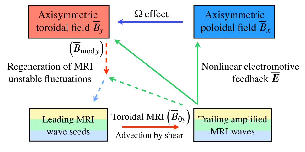
Figure 2: (Color online) Suggested physical mechanism of the MRI dynamo. Full arrows: main dynamo loop. Dashed arrows: nonlinear regeneration of MRI-unstable fluctuations. The various colors are used to identify the active modes taking part in the cyclic MRI dynamo described in Fig. 5: red (top left box) and blue (top right box) denote axisymmetric field components, different colors in the bottom boxes denote successive non-axisymmetric MRI waves.

Our goal to obtain sustained time-dependent MRI dynamo action in direct numerical simulations was to excite a dynamo loop involving the first two terms on the r.h.s. of Eq. (8), as depicted in Fig. 2. To do so, we first attempted to start from a very simple class of initial conditions combining

1. a “large-scale”, axisymmetric poloidal magnetic field $\overline{B}_{0x}$ (blue box in Fig. 2) whose stretching by the shear (“$\Omega$ effect", full line blue arrow in Fig. 2) produces an MRI-unstable axisymmetric toroidal field $\overline{B}_{0y}$ (red box in Fig. 2),

2. non-axisymmetric perturbations subject to joint amplification (full line red arrow in Fig. 2) by a transient toroidal MRI Balbus and Hawley (1992); Ogilvie and Pringle (1996); Terquem and Papaloizou (1996); Lesur and Ogilvie (2008b) of $\overline{B}_{0y}$ and by a kinematic Orr mechanism (swing amplification of non-axisymmetric waves, see Refs. Orr (1907); Butler and Farrell (1992); Johnson (2007)). These perturbations were chosen in the form of real random shearing wave packets with a full spectrum of $k_{z}$ and a single “horizontal” wavenumber pair $(k_{x}^{(0)}$, $k_{y})=\pm(-2\,\pi/L_{x},2\,\pi/L_{y})$ with leading ($k_{x}^{(0)}\,k_{y}<0$) polarization (different colors in the bottom left box of Fig. 2 represent successive individual leading waves). In the course of their evolution, such perturbations may generate a nonlinear electromotive feedback $\overline{\boldsymbol{E}}_{0}$ with the ability to sustain $\overline{\boldsymbol{B}}_{0}$ (full line green arrows in Fig. 2), thereby closing the main dynamo loop.

It turns out that, independently of the initial amplitudes of each of these perturbations, this restricted class of initial conditions can only trigger transient, short-lived dynamics. As explained in Sect. II.3, non-axisymmetric perturbations with a single initial horizontal wavenumber ($k_{x}^{(0)}$, $k_{y}$) can only be amplified for a few shearing times before they get sheared into a strongly trailing ($k_{x}(t)\,k_{y}\gg 0$, bottom right box with multiple colors in Fig. 2), rapidly decaying structure (Lesur and Ogilvie, 2008b). Besides, their nonlinear self-interaction cannot give rise to new non-axisymmetric leading waves, making it impossible to sustain $\overline{\boldsymbol{B}}_{0}$ against ohmic diffusion on long times. Hence, long-lived dynamics can only be excited if a distinct physical mechanism operates that generates new leading, transiently MRI-unstable perturbations. Exploring this issue, we then found that much longer-lived dynamics is obtained as soon as

• an $x$-dependent axisymmetric modulation

  $$\overline{\boldsymbol{B}}_{\mathrm{mod}}(x,z,t)=\overline{\boldsymbol{B}}_{\mathrm{mod}}(t)\cos\left(2\pi x/L_{x}\right)\cos\left(k_{z0}z\right)$$ (9)

  of $\overline{\boldsymbol{B}}$ is initially added on top of $\overline{\boldsymbol{B}}_{0}$, i.e.

  $$\overline{\boldsymbol{B}}(x,z,t=0)=\overline{\boldsymbol{B}}_{0}(z,t=0)+\overline{\boldsymbol{B}}_{\mathrm{mod}}(x,z,t=0)~{}.$$ (10)

This simple numerical observation indicated that the physical mechanism by which new leading shearing waves are generated requires that $\overline{\boldsymbol{B}}$ be modulated along the $x$ direction. The physical explanation for this behaviour is rather subtle, though : such a modulation of $\overline{\boldsymbol{B}}$ confines MRI-unstable perturbations in $x$ and allows for reflections of non-axisymmetric waves, somehow taking on the role of walls in a wall-bounded shear flow (non-axisymmetric instabilities in wall-bounded shear flows take on the form of global standing modes, see e.g. Ref. Waleffe (1997)). In more mathematical terms, the nonlinear triad interaction (shown by dashed arrows in Fig. 2) of the “confining” (say with $k_{x}=-2\pi/L_{x},k_{y}=0$) axisymmetric mode $\overline{\boldsymbol{B}}_{\mathrm{mod}}$ (red dashed arrow) with a trailing shearing wave (say $k_{x}(t)=\pi/L_{x}$, $k_{y}=2\pi/L_{y}$, green dashed arrow) can seed a new leading $(k_{x}(t)=-\pi/L_{x}$, $k_{y}=2\pi/L_{y})$ wave (light blue dashed arrow). This type of mechanism, which has long been suspected to be at work in non-rotating hydrodynamic shear flow turbulence (see for instance the discussion in Ref. (Farrell and Ioannou, 1993)) and has more recently been invoked in the context of hydrodynamic stability of accretion disks (Lithwick, 2007), is in fact essential to any sustained non-axisymmetric dynamics in the shearing box. We did check that the seeding of new leading waves in the simulations was not related to our implementation of the remap procedure (see Sect. II.3 and Ref. Umurhan and Regev (2004)), but had a genuine physical origin. In particular, the fact that long-lived dynamics and new leading waves can only be excited in the simulations if a $\overline{\boldsymbol{B}}_{\mathrm{mod}}$ component is added to the initial condition demonstrates that our numerical method does not artificially inject energy into leading waves.

To summarize this paragraph, using various relative combinations of axisymmetric and non-axisymmetric initial conditions composed of $\overline{\boldsymbol{B}}_{0}$, $\overline{\boldsymbol{B}}_{\mathrm{mod}}$ and a random leading shearing wave packet, we found it possible to obtain long-lived MRI dynamo action in direct shearing box simulations for different regimes. Based on these experiments, we claim that the essence of the driving mechanism of the MRI dynamo can be fully explained in terms of the few generic physical mechanisms described above and in Figure 2. As will be shown below, this claim is well supported by the targeted numerical experiment presented in Sect. IV.

III.2 Simplifying the dynamics

Approaching nonlinear cycles by DNS finally required us to find regions of parameter space in which only a small number of these structures are present. The dynamics in regimes ($\mathrm{Re}$, $\mathrm{Rm}$ of a few thousands) typical of simulations displaying pseudo-cyclic dynamics (Brandenburg et al., 1995; Lesur and Ogilvie, 2008a; Davis et al., 2010) being complex and probably involving a lot of different coherent structures, we restricted our investigations to $\mathrm{Re}$, $\mathrm{Rm}$ of a few hundreds. In such regimes, however, shearing waves are quickly damped after they turn trailing, unless $k_{x}(t)$ changes on a timescale much longer than $S^{-1}$. Exciting long-lived dynamics in this $\mathrm{Re}$ and $\mathrm{Rm}$ regime therefore further required setting $L_{y}\gg L_{x}$ ($|k_{y}|\ll|k_{x}^{(0)}|$ in Eq. (4)). Starting from various non-symmetric initial conditions, we then spotted that nonlinear states approaching a symmetry $\mathcal{A}_{1}$ (Nagata, 1986) of the shearing box MHD equations were regularly excited in DNS. This symmetry, described in the Appendix, allows for a large-scale axisymmetric magnetic field with the symmetry of $\overline{\boldsymbol{B}}_{0}$. In order to isolate these structures more easily, we then enforced numerically that the dynamics take place in the corresponding invariant subspace. This strategy was sufficient to excite recurrent dynamics in a large aspect ratio shearing box with $(L_{x},L_{y},L_{z})=(0.7,20,2)\,L$ and $\mathrm{Re}=70$, $\mathrm{Rm}=360$. A projection in the $\overline{B}_{0x}-\overline{B}_{0y}$ plane of a DNS trajectory approaching a nonlinear cycle in this regime is depicted in Fig. 3. The trajectory is seen to approach a periodic orbit after a few tens of shearing times and then to stay close to it for several hundred shearing times.

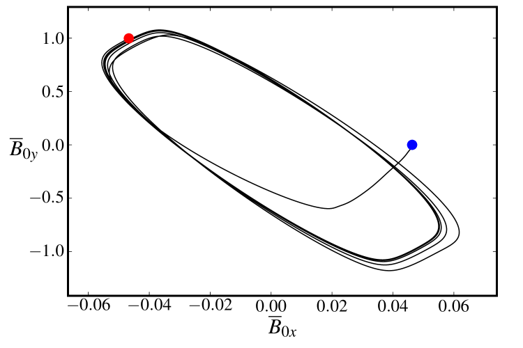
Figure 3: (Color online) Projection in the $\overline{B}_{0x}-\overline{B}_{0y}$ plane of a DNS trajectory approaching a nonlinear cycle for $(L_{x},L_{y},L_{z})=(0.7,20,2)\,L$ and $\mathrm{Re}=70$, $\mathrm{Rm}=360$. The full blue circle whose coordinates are $(0.046,0)$ marks the position of the system at $t=0$ and the red one located at $(-0.046,0.997)$ marks the position at $t=457.1\,S^{-1}$. Typical amplitudes of the various components of the initial conditions used to obtain this kind of trajectory are given in Sect. III.3.

III.3 Sensitive dependence on initial conditions

Before we close this Section, we find it necessary to emphasize that the dynamical system at hand has a very high sensitivity on initial conditions. This feature seems to be a very common property of shear flow turbulence (see for instance Ref. Faisst and Eckhardt (2004) for the case of hydrodynamic turbulence in pipe flow) and was explicitly demonstrated for the MRI dynamo problem in Ref. Rempel et al. (2010). In the course of this work, we clearly observed that the set of initial conditions leading to long-lived dynamics for the system at hand is fractal. For this reason, any statement of a set of precise numerical values for the amplitudes of the various types of perturbations involved in the design of the initial conditions leading to pseudo-cyclic dynamics is rather pointless. The problem is that different numerical codes, initialized exactly in the same way, will almost certainly diverge after a few shearing times because their algorithms will generate different numerical “noise” (low amplitude numerical errors) at each time step, subsequently leading to a rapid divergence (between different codes and also possibly different computer architectures) of phase-space trajectories such as that shown in Fig. 3. The initial amplitudes and relative mixtures of modes required to approach nonlinear cycles are therefore in the end specific to the numerical methods used in the code (this does not imply that the cyclic nonlinear solutions are not themselves robust, as discussed in the next Section). The only relevant helpful information for a reader eager to reproduce the results presented in Sect. IV and trajectories similar to that shown in Fig. 3 is a set of approximate values for the amplitudes of the perturbations entering our class of initial conditions, around which we found it possible to excite recurrent dynamics for $(L_{x},L_{y},L_{z})=(0.7,20,2)\,L$ and $\mathrm{Re}=70$ and $\mathrm{Rm}=360$: $\overline{B}_{0x}\simeq 0.046SL$, $\overline{B}_{\mathrm{mod\,y}}\simeq 0.11SL$, and non-axisymmetric shearing wave packets (with random relative amplitudes for different $k_{z}$, as described earlier) with comparable velocity and magnetic amplitudes of the order $0.3SL$.

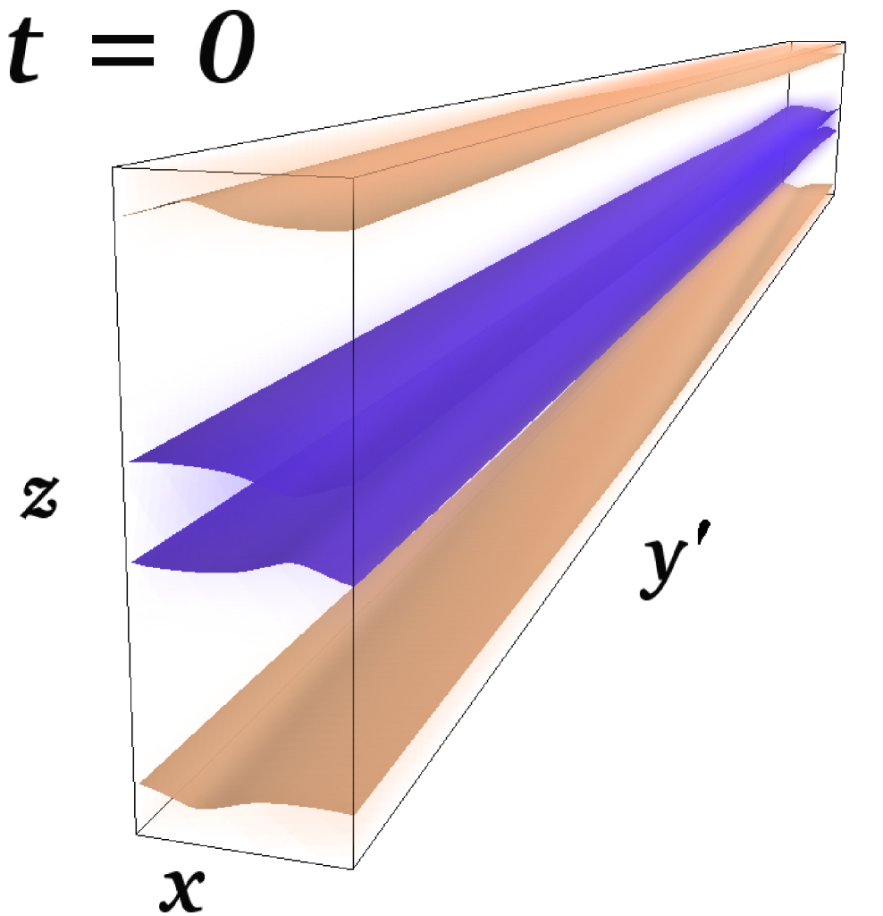
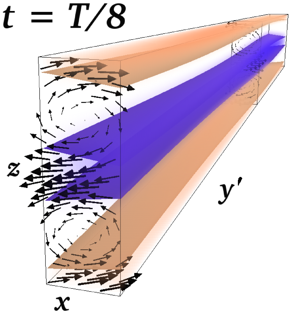
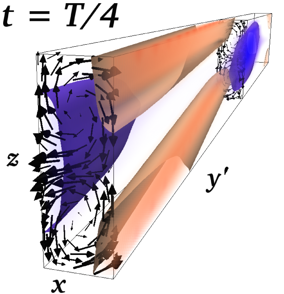
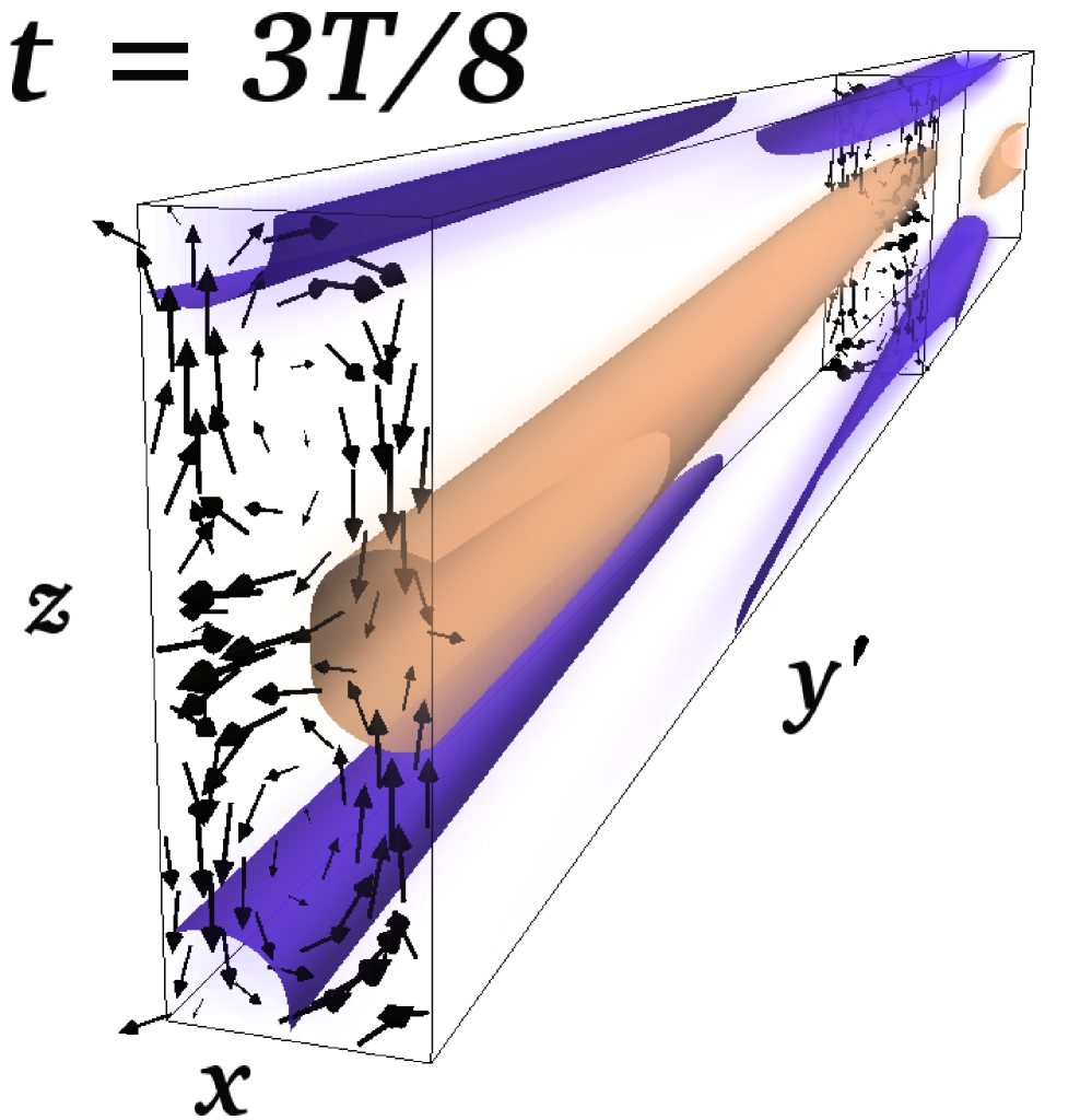
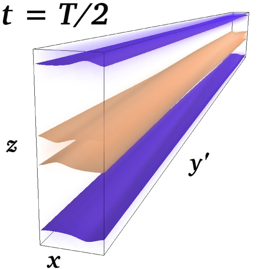
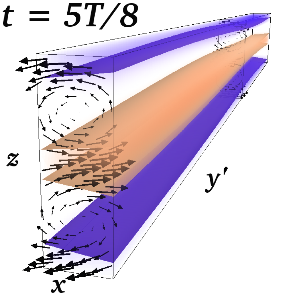
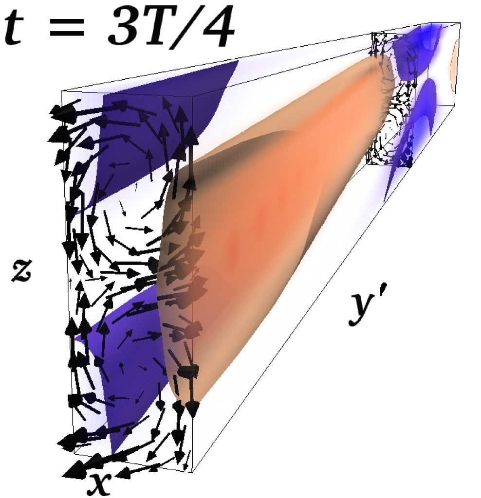
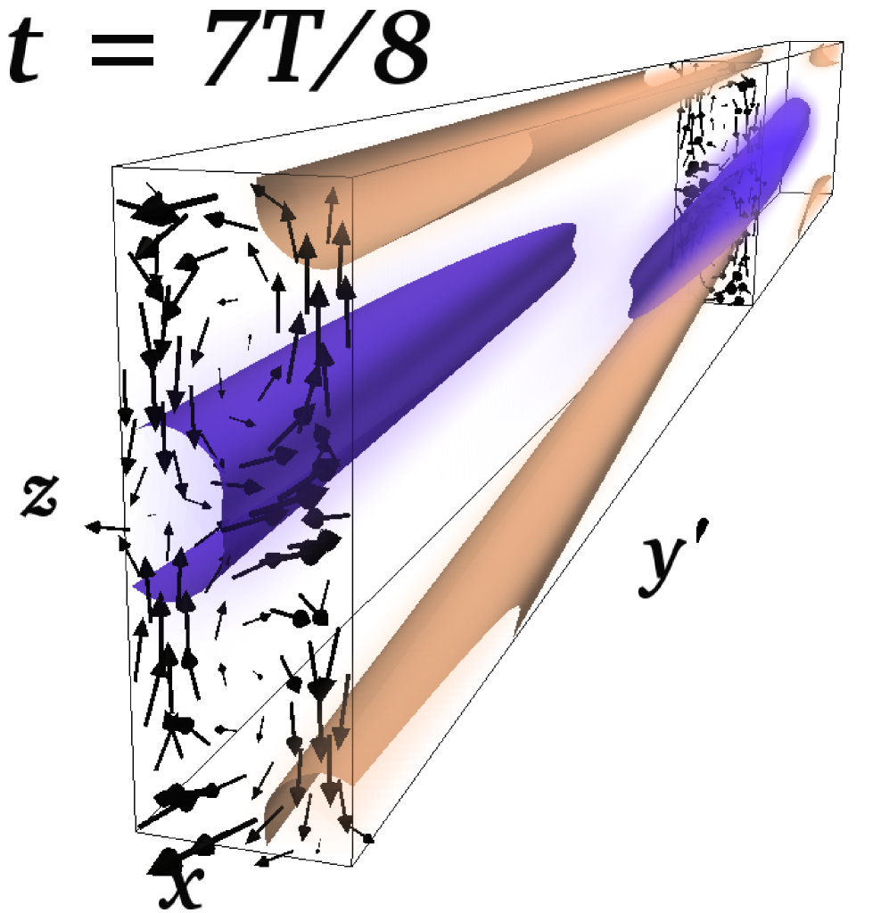
Figure 4: (Color online) Volume renderings of $B_{y}$ and isosurfaces of $B=0.9$ colored by $B_{y}$ every $T/8$ (positive $B_{y}$ in red/light gray, negative $B_{y}$ in blue-violet/dark gray). The coordinates of the bottom left corner of each box are $x=0$, $y^{\prime}=0$, $z=0$, where the $y^{\prime}$ coordinate is defined as $y^{\prime}=y-(L_{x}/2)St$ (see Appendix). The arrows field in the $y^{\prime}=0$ plane traces non-axisymmetric MRI velocity perturbations (velocity perturbations in the $y^{\prime}=L_{y}/2$ plane have opposite sign), whose effect is to distort and advect magnetic field lines of opposite polarities in opposite directions.

IV A nonlinear MRI dynamo cycle

Following the strategy defined in Sect. II.2, we then attempted to capture precisely the nonlinear cycle underlying the recurrent dynamics spotted in Fig. 3 using the Newton-Krylov solver PEANUTS.

IV.1 Convergence with Newton’s method

Because of shearing-periodic boundary conditions, only cycles whose period is a multiple of $L_{y}/(SL_{x})$ are allowed in shearing boxes. The periodicity of the recurrent dynamics spotted in the DNS being very close to $T=2\,L_{y}/(SL_{x})\simeq 57.143\,S^{-1}$, this period was imposed on the Newton solver. Initializing the solver with a snapshot of a DNS displaying dynamical recurrences (the red full circle point of Fig. 3), we obtained convergence to a cycle after $O(10)$ iterations with a relative error of $10^{-8}$. Each Newton step requires $O(10)$ Krylov iterations to solve the Jacobian system with a relative error smaller than $10^{-7}$. As each Krylov iteration requires running a DNS over a cycle period, $O(100)$ numerical integrations are needed to “capture” this cycle with this iterative method. The dynamics of this nonlinear MRI dynamo cycle is illustrated in Fig. 4. The results presented here are for a resolution $(N_{x},N_{y},N_{z})=(48,24,72)$ with 2/3 dealiasing (the same resolution used to approach the cycle by DNS). Half that resolution already ensures convergence to very good accuracy. Analyzing the energy spectrum of the cycle, we only found differences of a few percent between the full-resolution and half-resolution runs.

In respect of the observations made in Sect. III.3, we emphasize that the cycle calculated by the means of Newton’s method is not a spurious numerical feature. The most important requirement for convergence, as is standard with Newton’s algorithm, is that the DNS snapshot used as a starting guess for the algorithm be in close-enough vicinity of the cycle. Provided that this requirement is satisfied, convergence to the cycle is robust and can be obtained by using (as a starting guess for the Newton solver) various adequate DNS snapshots resulting from integrations of various sets of initial conditions, for various Courant-Friedrichs-Lewy conditions for the numerical time-integrator, using either fixed or adaptative time-stepping.

Finally, it is important to stress that the cycle at hand is a genuine solution to the full discretized nonlinear 3D MHD equations in the shearing box, not just a solution to a low-dimensional, reduced dynamical model of the problem. The imposition of symmetries in the numerical resolution only helps to target nonlinear cycles with a given natural symmetry (i.e. a symmetry allowed by the full MHD equations in the geometry studied) more easily. In fact, once convergence is achieved with the Newton solver, the cycle can be integrated for several periods in a standard DNS without enforcing any symmetry.

IV.2 Description of the cycle

The physics of the cycle is best understood by looking at Fig. 4. A large-scale axisymmetric toroidal field $\overline{B}_{y}$ with $z$-dependent polarity dominates at $t=0$. The MRI mediated by that field progressively amplifies weak, leading non-axisymmetric perturbations. The effect of the instability is to separate “radially” (in $x$) fluid particles initially attached to individual, almost frozen-in field lines (Balbus and Hawley, 1998), leading to their non-axisymmetric distortion ($T/8$ to $T/4$). In addition, for the cycle at hand, linear MRI velocity perturbations drag fields lines with opposite polarities in opposite directions. As they get sheared, MRI-amplified velocity perturbations take the form of a non-axisymmetric pattern of counter-rotating poloidal flow cells. The $z$ component of the flow advects distorted magnetic field lines with opposite polarities in opposite $z$ directions, effectively reversing regions of positive and negative polarities ($T/4$). The $x$ component of the cellular flow eventually advects field lines back to their original $x$ location ($3T/8$), producing at $T/2$ an axisymmetric magnetic field opposite to the original one. Hence, the reversal is the pure outcome of the nonlinear evolution (self-interactions) of non-axisymmetric MRI perturbations. As a result of the confinement of MRI perturbations by the shearwise-modulated MRI-supporting toroidal field, new leading perturbations seeds are generated during the first half of the cycle. Their subsequent amplification and nonlinear evolution during the second half of the cycle result in a new field reversal after another $T/2$, back to the initial state.

This qualitative physical scenario is fully supported by a quantitative analysis of the time-evolution (Fig. 5). The linear MRI of the $z$-dependent axisymmetric toroidal field $\overline{B}_{0y}$ (Fig. 5a in red) amplifies successive non-axisymmetric shearing MRI waves (Fig. 5d, rainbow colors) with $k_{y}=\pm 2\pi/L_{y}$ and a $k_{z}$ spectrum. The nonlinear self-interaction of a single wave packet translates into an axisymmetric EMF $\overline{\boldsymbol{E}}_{0}$ whose $x$ and $y$ components are clearly responsible for the reversals of $\overline{\boldsymbol{B}}_{0}$ (Fig. 5b). Interestingly, a calculation of the various terms on the r.h.s. of the projection of Eq. (8) on $\boldsymbol{e}_{y}$ throughout the cycle shows that the $\Omega$ effect is not the dominant term in this equation for this particular cycle and geometry (Fig. 5c). Hence, $\overline{B}_{0x}$ and $\overline{B}_{0y}$ are almost in antiphase, whereas they are almost in quadrature for the pseudo-cycle described in Ref. Lesur and Ogilvie (2008a). Fig. 5d clearly demonstrates the periodic seeding of new leading perturbations (yellow, green, light blue etc. represent successive shearing waves, as in Fig. 2). The evolution of the amplitude of $\overline{B}_{\mathrm{mod}\,y}$, defined in Eq. (9), is depicted in Fig. 5e. $\overline{B}_{\mathrm{mod}\,y}$ is very small compared to $\overline{B}_{0y}$, which demonstrates that a very weak confinement of the MRI is actually sufficient to generate new leading waves.

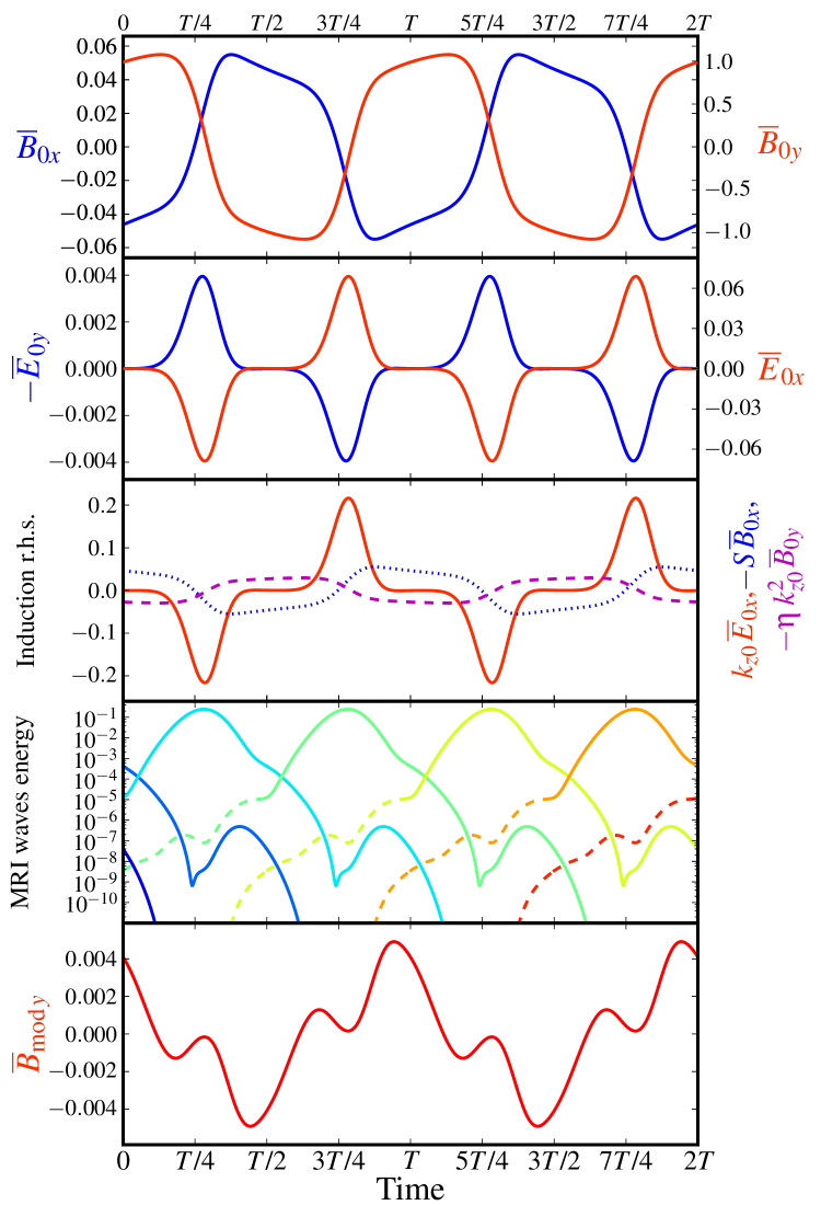
Figure 5: (Color online) From top to bottom: evolution over two cycles of a) $\overline{B}_{0x}$ (blue/dark gray) and $\overline{B}_{0y}$ (red/light gray) ; b) $-\overline{E}_{0y}$ (blue/dark gray, source term for $\overline{B}_{0x}$) and $\overline{E}_{0x}$ (red / light gray, source term for $\overline{B}_{0y}$) ; c) amplitudes of the three terms on the r.h.s. of the projection of the axisymmetric induction Eq. (8) on $\boldsymbol{e}_{y}$ (dotted blue: $\Omega$ effect, full line red: nonlinear EMF, dashed magenta: magnetic diffusion) ; d) total energy of successive MRI shearing waves with $k_{y}=\pm 2\pi/L_{y}$ (rainbow colors, dashed/full line: leading/trailing phase. Each color represents a different shearing wave) ; e), amplitude of the axisymmetric magnetic field modulation $\overline{B}_{\mathrm{mod}\,y}$.

As seen in Fig. 4, the reason why such a cycle can be computed at fairly low resolutions (in particular in the $y$ direction) is that it is a large-scale, time-dependent coherent structure whose non-axisymmetric dynamics (and the corresponding axisymmetric dynamo feedback $\overline{\boldsymbol{E}}_{0}$ that it induces) is largely dominated by MRI shearing waves supported by the fundamental Fourier mode $k_{y}=2\pi/L_{y}$ of the shearing box in the $y$ direction. We also note that all the physical processes involved are not actually specific to the shearing box, and may therefore also be present in cylindrical geometry, with non-axisymmetric perturbations taking on the form of sheared spiral waves.

Finally, remark that the energy required to sustain the three-dimensional cyclic dynamics against resistive and viscous dissipation is extracted from the shear (which is the only available energy source of the system) thanks to the toroidal MRI of non-axisymmetric shearing waves.

IV.3 Stability

Using the Floquet eigenvalue solver, we found that the cycle has a single unstable eigenmode, with a Floquet eigenvalue $\Lambda\simeq 32.33$ corresponding to a positive growth rate $\lambda=\ln\Lambda/T\simeq 0.061\,S$ (at half resolution, $\Lambda=22.63$, $\lambda\simeq 0.055\,S$), and the same $\mathcal{A}_{1}$ symmetry. Hence, any small perturbation to the cycle, independently of its initial amplitude, ultimately kicks the system out of its initially periodic trajectory in phase-space. This exponential instability of the cycle was observed in the simulations and leads to complete escape from the neighbourhood of the cyclic solution after a few hundred shearing times. Unstable periodic orbits such as this one are a typical feature of chaotic dynamical systems and play an important role in their dynamics (see discussion in Sect. V).

IV.4 Investigating the nature of dynamo action

One may finally wonder if the nonlinear couplings leading to this dynamo can be described by standard mean-field theory. $\alpha^{2}$ or $\alpha\Omega$ dynamos are ruled out: both net kinetic and current helicities are negligible in the DNS. For our cycle, the axisymmetric field and EMF are largely dominated by their projection $\overline{\boldsymbol{B}}_{0}$ and $\overline{\boldsymbol{E}}_{0}$ on $\cos(2\pi z/L_{z})$ and $\sin(2\pi z/L_{z})$ planforms (see Eqs. (6)-(7)), so one may be tempted to interpret the dynamo feedback in terms of a non-diagonal “turbulent resistivity” $\bar{\bar{\eta}}$ tensor (Gressel, 2010) that would couple the amplitudes of the components of $\overline{\boldsymbol{B}}_{0}$ and $\overline{\boldsymbol{E}}_{0}$ linearly. However, not only is the instantaneous relationship between these two quantities unambiguously nonlinear (Fig. 6), it also looks rather difficult to model analytically based on simple physical arguments. Hence, this periodic MRI dynamo does not reduce to a simple standard mean-field dynamo, a conclusion that also seems to apply to the magnetic buoyancy-driven dynamo (Cline et al., 2003; Davies and Hughes, 2011).

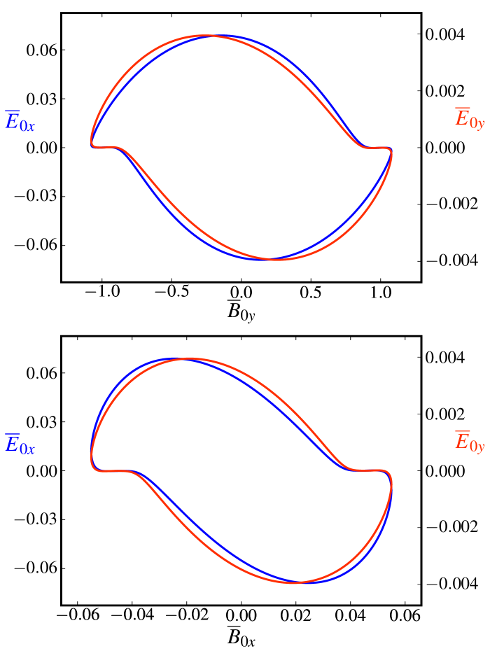
Figure 6: (Color online) Projection of the periodic MRI dynamo orbit in the $\overline{E}_{x}$ (blue/dark gray) | $\overline{E}_{y}$ (red/light gray) vs. $\overline{B}_{x}$ | $\overline{B}_{y}$ planes.

V Discussion and conclusions

We have presented the first accurate numerical determination of a cyclic nonlinear MRI dynamo solution to the original 3D dissipative incompressible MHD equations in the regime of Keplerian differential rotation. Preliminary investigations indicate that its existence is not limited to a narrow range of $\mathrm{Re}$ and $\mathrm{Rm}$, unlike the plane Couette flow stationary solution reported in Ref. Rincon et al. (2007), and may notably extend down to low magnetic Prandtl number regimes in which recent studies have found it difficult to obtain sustained MRI dynamo turbulence (Fromang et al., 2007). A detailed parametric study of the cycle and an assessment of its importance for the MRI dynamo transition problem is currently underway and will be presented in a separate paper.

Overall, the discovery of this MRI dynamo limit cycle significantly extends and consolidates earlier findings (Rincon et al., 2007) and claims (Rincon et al., 2008; Rempel et al., 2010) that dynamo action and MHD turbulence in shear flows prone to local MHD instabilities has a similar nature to hydrodynamic turbulence in shear flows. The results notably provide clear evidence that magnetic field generation and sustenance at moderate $\mathrm{Re}$, $\mathrm{Rm}$ in a numerical set-up comparable to that of most MRI dynamo simulations so far results from a nonlinear mechanism of interaction between axisymmetric fields and non-axisymmetric instability modes. The detailed description of the process may guide future studies of dynamos mediated by MHD instabilities other than the MRI (Spruit, 2002; Cline et al., 2003; Braithwaite, 2006; Miesch et al., 2007; Tobias et al., 2011).

Our findings also demonstrate that new theoretical models of large-scale dynamo action are required. Progress on this problem may be possible thanks to periodic orbit theory (Cvitanovic, 1992), which offers formal mathematical connections between the statistical properties of dynamical systems with a small number of active degrees of freedom and their unstable cycles. One should therefore attempt to identify new MRI dynamo cycles, analyze their dependence on various parameters and assess their relative dynamical importance using stability analysis. It is almost certain that, similarly to hydrodynamic shear flows (Viswanath, 2007), many such structures exist in the phase space of MHD-unstable shear flows at moderate and large $\mathrm{Re}$ and $\mathrm{Rm}$.

This approach may also prove useful for the astrophysics problem of turbulent transport of angular momentum in accretion disks (Balbus and Hawley, 1998). The fact that the MRI dynamo cycle described above generates an average turbulent MHD stress $\alpha\sim 0.025\,(SL)^{2}$ directly comparable to that obtained in direct numerical simulations of similar configurations (Fromang et al., 2007) constitutes a notable preliminary finding in this respect.

We finally point out that the MHD findings reported in this study, which have partly been inspired by recent advances in the field of shear flow hydrodynamics, may in return be helpful to make progress on understanding hydrodynamic shear flow turbulence. The leading wave regeneration mechanism that was clearly identified in the shearing box in this work offers an interesting connexion between three-dimensional turbulence in wall-bounded and homogeneous shear flows, which may notably help to understand if regeneration pseudo-cycles in the latter (see e.g. Ref. (Gualtieri et al., 2002)) share a common physical origin with nonlinear cycles in wall-bounded shear flows (Viswanath, 2007).

*

Appendix A Symmetries

Nagata (Nagata, 1986) identified several possible symmetries for three-dimensional nonlinear hydrodynamic solutions in centrifugally unstable (Rayleigh-unstable) Taylor-Couette flow in the thin-gap limit, which corresponds to a cartesian plane Couette flow with walls, rotating along its spanwise $z$ axis. These symmetries can be adapted to the shearing box and generalized to MHD flows.

We consider a physical domain with $0\leq x<L_{x}$, $0\leq y<L_{y}$ and $0\leq z<L_{z}$. For visualization purposes, we assume that the observer is comoving with the base flow at $x=L_{x}/2$ and therefore introduce

$$y^{\prime}=y-\frac{L_{x}}{2}St~{}.$$ (11)

In Fig. 4, the coordinates of the lower left corner of each box are $x=0$, $y^{\prime}=0$, $z=0$. The various fields entering the nonlinear dynamo cycle solution presented in this paper have the following generalized $\mathcal{A}_{1}$ symmetry:

$$\boldsymbol{u}:\left\{\begin{array}[]{lllll}u_{x}&=&u_{x,\mathrm{e}\mathrm{e}}(t)\cos\left(k_{z\mathrm{e}}z\right)\sin\left(k_{y\mathrm{e}}y^{\prime}+k_{x}(t)x\right)&+&u_{x,\mathrm{o}\mathrm{o}}(t)\cos\left(k_{z\mathrm{o}}z\right)\cos\left(k_{y\mathrm{o}}y^{\prime}+k_{x}(t)x\right)\\ u_{y}&=&u_{y,\mathrm{e}\mathrm{e}}(t)\cos\left(k_{z\mathrm{e}}z\right)\sin\left(k_{y\mathrm{e}}y^{\prime}+k_{x}(t)x\right)&+&u_{y,\mathrm{o}\mathrm{o}}(t)\cos\left(k_{z\mathrm{o}}z\right)\cos\left(k_{y\mathrm{o}}y^{\prime}+k_{x}(t)x\right)\\ u_{z}&=&u_{z,\mathrm{e}\mathrm{e}}(t)\sin\left(k_{z\mathrm{e}}z\right)\cos\left(k_{y\mathrm{e}}y^{\prime}+k_{x}(t)x\right)&+&u_{z,\mathrm{o}\mathrm{o}}(t)\sin\left(k_{z\mathrm{o}}z\right)\sin\left(k_{y\mathrm{o}}y^{\prime}+k_{x}(t)x\right)\end{array}\right\}~{},$$ (12)

$$\boldsymbol{B}:\left\{\begin{array}[]{lllll}B_{x}&=&B_{x,\mathrm{e}\mathrm{o}}(t)\cos\left(k_{z\mathrm{e}}z\right)\sin\left(k_{y\mathrm{o}}y^{\prime}+k_{x}(t)x\right)&+&B_{x,\mathrm{o}\mathrm{e}}(t)\cos\left(k_{z\mathrm{o}}z\right)\cos\left(k_{y\mathrm{e}}y^{\prime}+k_{x}(t)x\right)\\ B_{y}&=&B_{y,\mathrm{e}\mathrm{o}}(t)\cos\left(k_{z\mathrm{e}}z\right)\sin\left(k_{y\mathrm{o}}y^{\prime}+k_{x}(t)x\right)&+&B_{y,\mathrm{o}\mathrm{e}}(t)\cos\left(k_{z\mathrm{o}}z\right)\cos\left(k_{y\mathrm{e}}y^{\prime}+k_{x}(t)x\right)\\ B_{z}&=&B_{z,\mathrm{e}\mathrm{o}}(t)\sin\left(k_{z\mathrm{e}}z\right)\cos\left(k_{y\mathrm{o}}y^{\prime}+k_{x}(t)x\right)&+&B_{z,\mathrm{o}\mathrm{e}}(t)\sin\left(k_{z\mathrm{o}}z\right)\sin\left(k_{y\mathrm{e}}y^{\prime}+k_{x}(t)x\right)\end{array}\right\}~{},$$ (13)

where the $\mathrm{e}$ and $\mathrm{o}$ subscripts indicate that the associated discrete wavenumbers are based on even and odd relative integers, respectively. $k_{x}(t)$ in each individual trigonometric expression is defined implicitly by Eq. (4) using the $k_{y}$ wavenumber of the same expression. It can be checked that this symmetry is conserved by the MHD equations (1)-(3). When needed, we enforced numerically that the dynamical evolution took place in the invariant subspace defined by this symmetry by imposing it in the initial conditions and by further enforcing it every shearing time during the numerical integrations in order to avoid the growth of non-symmetric numerical noise.