Incomplete current fluctuation theorems for a four-terminal model

Abstract

We demonstrate the validity of the current fluctuation theorem for a double quantum dot surrounded by four terminals within the Born-, Markov- and secular approximations beyond the Coulomb-blockade regime. The electronic tunneling to two fermionic contacts conserves the total number of electrons, and the internal tunneling is phonon-assisted by two bosonic baths. Adapted choice of thermodynamic parameters between the baths may drive a current against an existing electric or thermal gradient. We study the apparent violation of the fluctuation theorem when only some of the energy and matter currents are monitored.

Fluctuation theorems (FTs) connect forward and backward probabilities for processes associated with a definite exchange of entropy seifert2005a . Thereby they relate rather sophisticated and hard-to-calculate quantities with simple and universal thermodynamic parameters, which constitutes part of their attractiveness. When the matter and energy currents are tracked over a certain period of time, there exist simple versions of the current (or Full Counting Statistics) FT andrieux2004a ; andrieux2006a ; andrieux2009a ; esposito2007b . Significant progress made in the monitoring of electronic tunneling events through quantum dots (QDs) gustavsson2006a ; sukhorukov2007a by using capacitively coupled quantum point contacts (QPCs) has led to an accurate understanding of Full Counting Statistics flindt2009a . Unfortunately, the QPC signal originating from a monitored single dot does not allow to reconstruct bi-directional tunneling events. Therefore, monitored double quantum dots allowing for bi-directional counting have entered the focus of interest fujisawa2006a ; utsumi2010a and appear as ideal testbeds to check current FTs.

It is therefore essential to identify processes that may lead to modifications of the FT in an experimental setup. The FT has been found to be modified due to true quantum effects such as Berry phases ren2010a or interference effects saito2008a ; foerster2008a ; utsumi2009a . It may however also be modified due to detector back-action – e.g., the back-action of QPC on a monitored double quantum dot golubev2011a ; kueng2011a or the influence of a single electron transistor monitoring another one sanchez2010a ; bulnes_cuetara2011a – or simply when detailed balance is explicitly broken via feedback control schaller2011b .

Here, we will argue at the example of phonon-assisted tunneling that an apparent violation of the current FT may also arise due to ignored couplings with further baths (that might resist an experimental monitoring).

This paper is organized as follows: In Sec. I we introduce our model and the method, followed by a verification of the multi-terminal FT in Sec. II. We discuss how the multi-terminal FT is modified when only partial information is available in Sec. III.

I Model and Methods

I.1 Hamiltonian

We consider a double quantum dot system (see Fig. 1)

$$\mathcal{H}_{\rm S}=\upvarepsilon_{\rm A}d_{\rm A}^{\dagger}d_{\rm A}+\upvarepsilon_{\rm B}d_{\rm B}^{\dagger}d_{\rm B}+Ud_{\rm A}^{\dagger}d_{\rm A}d_{\rm B}^{\dagger}d_{\rm B}$$ (1)

with on-site energies $\upvarepsilon_{\rm A}$ and $\upvarepsilon_{\rm B}$ and Coulomb-interaction $U$.

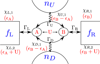
Figure 1: (Color online) Two quantum dots $A$ and $B$ are tunnel-coupled to adjacent fermionic contacts described by Fermi-distributions $f_{L}$ and $f_{R}$ with rates $\Gamma_{\rm L}$ and $\Gamma_{\rm R}$, respectively. Electronic transitions between the QDs are only possible in the singly-charged sector via spontaneous emission or absorption of a boson with energy transfer $\upvarepsilon_{\rm B}-\upvarepsilon_{\rm A}$ from upper or lower phonon baths (defined by Bose-Einstein distributions $n_{U}$ and $n_{D}$) with rates $\Gamma_{\rm U}$ and $\Gamma_{\rm D}$. We explicitly allow for double occupation of the system, such that the coupling between particles and energy transferred to the fermionic reservoirs is not tight: Depending on whether the inert QD is occupied or not, the energy exchanged (red, in brackets) with the fermionic baths may vary. The use of multiple particle counting fields specific to both reservoir and transferred energy facilitates the calculation of the complete particle-energy counting statistics.

Without loss of generality (mirror symmetry) we assume that $\upvarepsilon_{\rm A}<\upvarepsilon_{\rm B}$. The system is surrounded by two bosonic $\sigma\in\{U,D\}$ and two fermionic $\alpha\in\{L,R\}$ baths

$$\mathcal{H}_{\rm B}=\sum_{k,\alpha}\upvarepsilon_{k,\alpha}c_{k,\alpha}^{\dagger}c_{k,\alpha}+\sum_{k,\sigma}\omega_{k,\sigma}b_{k,\sigma}^{\dagger}b_{k,\sigma}\,,$$ (2)

that are assumed to remain in thermal equilibrium throughout. Each QD is coupled to its adjacent fermionic contact by the tunneling Hamiltonian

$$\mathcal{H}_{\rm I}^{\rm el}=d_{\rm A}\sum_{k}t_{k,\rm L}c_{k,\rm L}^{\dagger}+d_{\rm B}\sum_{k}t_{k,\rm R}c_{k,\rm R}^{\dagger}+{\rm h.c.}\,,$$ (3)

where the tunneling amplitudes $t_{k,\alpha}$ lead to effective tunneling rates $\Gamma_{\alpha}\equiv\Gamma_{\alpha}(\omega)=2\pi\sum_{k}{\left|t_{k,\alpha}\right|}^{2}\delta(\omega-\upvarepsilon_{k,\alpha})$ that we assume to be energy independent (wideband limit). In contrast, the transition $A\leftrightarrow B$ is phonon-assisted via the interaction

$$\mathcal{H}_{\rm I}^{\rm ph}=(d_{\rm A}d_{\rm B}^{\dagger}+d_{\rm B}d_{\rm A}^{\dagger})\otimes\sum_{k,\sigma}(h_{k,\sigma}b_{k,\sigma}+h_{k,\sigma}^{\ast}b_{k,\sigma}^{\dagger})\,,$$ (4)

such that – under the rotating wave approximation – an electron jump between the QDs goes with either emission or absorption of a boson from upper or lower bath galperin2005a . We again summarize the corresponding amplitudes in effective energy-independent phonon-assisted electron tunneling rates $\Gamma_{\sigma}\equiv\Gamma_{\sigma}(\omega)=2\pi\sum_{k}{\left|h_{k,\sigma}\right|}^{2}\delta(\omega-\omega_{k,\sigma})$. The resulting total model is described by the sum of all Hamiltonians ${\mathcal{H}}=\mathcal{H}_{\rm S}+\mathcal{H}_{\rm B}+\mathcal{H}_{\rm I}^{\rm el}+\mathcal{H}_{\rm I}^{\rm ph}$ and is visualized in Fig. 1.

I.2 Liouvillian

We assume to be in the sequential tunneling regime, where second order perturbation theory in the couplings $t_{k\alpha}$ and $h_{k\sigma}$ to the contacts is a good approximation. This regime can e.g. be achieved when all tunneling rates are small in comparison to the reservoir temperatures $\Gamma_{\alpha/\sigma}\ll k_{\rm B}T_{\alpha/\sigma}$ koenig1996a ; emary2009a . More generally, Kondo physics is expected to be negligible when the reservoir temperatures are larger than the Kondo temperature garate2011a . In this regime, performing the Born, Markov, and secular approximations breuer2002 yields a master equation that is expected to yield valid results. It involves only the system density matrix, is of Lindblad-form lindblad1976a , and in the (localized) system energy eigenbasis ($\mathcal{H}_{\rm S}\left|00\right>=0$, $\mathcal{H}_{\rm S}\left|10\right>=\upvarepsilon_{\rm A}\left|10\right>$, $\mathcal{H}_{\rm S}\left|01\right>=\upvarepsilon_{\rm B}\left|01\right>$, and $\mathcal{H}_{\rm S}\left|11\right>=(\upvarepsilon_{\rm A}+\upvarepsilon_{\rm B}+U)\left|11\right>$) it assumes the form of a simple rate equation as long as the energy levels of $\mathcal{H}_{\rm S}$ are non-degenerate (recall that $\upvarepsilon_{\rm B}>\upvarepsilon_{\rm A}$). In principle, the rates may be calculated rigorously but the result is also evident from Fermis Golden rule. We assume the reservoirs to be in thermal equilibrium throughout, i.e., expectation values are given by the Fermi-Dirac

$$\left<c_{k,\alpha}^{\dagger}c_{k,\alpha}\right>\equiv f_{\alpha}(\varepsilon_{k,\alpha})=\frac{1}{e^{\beta_{\alpha}(\varepsilon_{k,\alpha}-\mu_{\alpha})}+1}$$ (5)

or Bose-Einstein

$$\left<b_{k,\sigma}^{\dagger}b_{k,\sigma}\right>\equiv n_{\sigma}(\omega_{k,\sigma})=\frac{1}{e^{\beta_{\sigma}(\omega_{k,\sigma}-\mu_{\sigma})}-1}$$ (6)

distributions, respectively, where $\beta_{\alpha}$ and $\beta_{\sigma}$ denote the inverse electronic or bosonic bath temperatures and $\mu_{\alpha}$ and $\mu_{\sigma}$ the respective chemical potentials. Writing the diagonal entries of the system density matrix in a vector $\rho_{\rm S}=(\rho_{00,00},\rho_{10,10},\rho_{01,01},\rho_{11,11})$, the master equation to this order assumes the form $\dot{\rho_{\rm S}}=\mathcal{L}\rho_{\rm S}$, where the Liouvillian superoperators are given by

$$\mathcal{L} = (\mathcal{L}_{\rm L}+\mathcal{L}_{\rm R}+\mathcal{L}_{\rm U}+\mathcal{L}_{\rm D})\,,$$

$$\mathcal{L}_{\rm L} = \Gamma_{\rm L}\begin{pmatrix}-f_{\rm L}&+(1-f_{\rm L})&0&0\\ +f_{\rm L}&-(1-f_{\rm L})&0&0\\ 0&0&-\bar{f}_{\rm L}&+(1-\bar{f}_{\rm L})\\ 0&0&+\bar{f}_{\rm L}&-(1-\bar{f}_{\rm L})\end{pmatrix}\,,$$

$$\mathcal{L}_{\rm R} = \Gamma_{\rm R}\begin{pmatrix}-f_{\rm R}&0&+(1-f_{\rm R})&0\\ 0&-\bar{f}_{\rm R}&0&+(1-\bar{f}_{\rm R})\\ +f_{\rm R}&0&-(1-f_{\rm R})&0\\ 0&+\bar{f}_{\rm R}&0&-(1-\bar{f}_{\rm R}\end{pmatrix}\,,$$

$$\mathcal{L}_{\rm\sigma} = \Gamma_{\sigma}\begin{pmatrix}0&0&0&0\\ 0&-n_{\sigma}&+(1+n_{\sigma})&0\\ 0&+n_{\sigma}&-(1+n_{\sigma})&0\\ 0&0&0&0\end{pmatrix}\,.$$ (7)

Here, we have used the abbreviations

$$n_{\sigma} \equiv n_{\sigma}(\upvarepsilon_{\rm B}-\upvarepsilon_{\rm A})\,,$$

$$f_{\rm L} \equiv f_{\rm L}(\upvarepsilon_{\rm A})\,,\qquad f_{\rm R}\equiv f_{\rm R}(\upvarepsilon_{\rm B})\,,$$

$$\bar{f}_{\rm L} \equiv f_{\rm L}(\upvarepsilon_{\rm A}+U)\,,\qquad\bar{f}_{\rm R}\equiv f_{\rm R}(\upvarepsilon_{\rm B}+U)\,,$$ (8)

compare Eqns. (5) and (6). In the Coulomb-blockade limit, the doubly occupied state always decays, which is formally expressed by the limits $\bar{f}_{L}\to 0$ and $\bar{f}_{R}\to 0$, and the top-left $3\times 3$ submatrix of the above equation reproduces previous models in the literature rutten2009a .

It should be noted that the above Liouvillian (I.2) only satisfies local detailed balance esposito2010a : When the system is only coupled to a single junction $\Sigma\in\{L,R,U,D\}$, detailed balance $\mathcal{L}^{k\ell}_{\Sigma}\bar{\rho}^{\ell}_{\Sigma}=\mathcal{L}^{\ell k}_{\Sigma}\bar{\rho}^{k}_{\Sigma}$ – where $\bar{\rho}^{k}_{\Sigma}$ denotes the corresponding single-junction stationary state – is obeyed. When it is coupled to all four terminals however, global detailed balance is broken.

I.3 Conditional Master Equation

Being responsible for transitions between different system states, the off-diagonal matrix elements of the Liouvillians in Eqns. (I.2) can be used to set up a connected set of equations for density matrices $\rho^{(n)}(t)$ conditioned upon the number of particles $n$ that have tunneled to a respective reservoir gurvitz1996a . That is, although the state of the system density matrix does neither yield information on the number of particles nor the energy transferred to a certain bath, the full time-record of a single trajectory would reveal this information. When we only focus on a single reservoir to and out of which we count all particle jumps, the conditioned density matrices follow an equation of the form $\dot{\rho}^{(n)}={\mathcal{L}}_{0}\rho^{(n)}+{\mathcal{L}}_{+}\rho^{(n-1)}+{\mathcal{L}}_{-}\rho^{(n+1)}$, where ${\mathcal{L}}_{+}$ (${\mathcal{L}}_{-}$) describes particle jumps into (out of) the reservoir of interest and ${\mathcal{L}}_{0}$ contains the remaining terms (jumps to and from other reservoirs as well as the diagonal matrix elements). Alternatively, such $n$-resolved master equations may also be obtained by performing the derivation after a detector has been added to the system schaller2009b . By performing a Fourier transform

$$\rho_{\rm S}(\chi,t)\equiv\sum_{n}\rho_{\rm S}^{(n)}(t)e^{\mathrm{i}n\chi}\,,$$ (9)

one can convert the infinitely large $n$-resolved, conditional master equation to a four-dimensional one at the price of introducing the counting field $\chi$. Being e.g. interested in the number of particles in the left contact, this formally corresponds to the replacements $f_{L}\to f_{L}e^{-i\chi}$ and $(1-f_{L})\to(1-f_{L})e^{+i\chi}$ in the off-diagonal matrix elements of Eqns. (I.2), respectively.

However, here we are interested in the full energy-particle counting statistics, such that one has to treat e.g. single-electron jumps corresponding to an energy change of $\upvarepsilon_{\rm A}$ and to an energy change of $\upvarepsilon_{\rm A}+U$ in the system differently. Therefore, we introduce two counting fields for each fermionic contact and one for each bosonic contact. Note that in the Coulomb-blockade limit, energy and particle fluxes are tightly coupled (often also called strongly coupled rutten2009a ), such that also for the fermionic contacts a single counting field would suffice. The Liouvillian as a function of energy-resolved counting fields reads

$$\mathcal{L}(\mbox{\boldmath$\chi$}) \equiv \mathcal{L}(\chi_{\rm L1},\chi_{\rm L2},\chi_{\rm R1},\chi_{\rm R2},\chi_{\rm U1},\chi_{\rm D1})$$ (10)

$$= \mathcal{L}_{\rm L}(\chi_{\rm L1},\chi_{\rm L2})+\mathcal{L}_{\rm R}(\chi_{\rm R1},\chi_{\rm R2})$$

$$+\mathcal{L}_{\rm U}(\chi_{\rm U1})+\mathcal{L}_{\rm D}(\chi_{\rm D1})\,,$$

where the explicit counting field dependence can be obtained from Eqns. (I.2) by performing the replacements

$$f_{\rm L} \to f_{\rm L}e^{-\mathrm{i}\chi_{\rm L1}}\,,\qquad(1-f_{\rm L})\to(1-f_{\rm L})e^{+\mathrm{i}\chi_{\rm L1}}\,,$$

$$\bar{f}_{\rm L} \to \bar{f}_{\rm L}e^{-\mathrm{i}\chi_{\rm L2}}\,,\qquad(1-\bar{f}_{\rm L})\to(1-\bar{f}_{\rm L})e^{+\mathrm{i}\chi_{\rm L2}}\,,$$

$$f_{\rm R} \to f_{\rm R}e^{-\mathrm{i}\chi_{\rm R1}}\,,\qquad(1-f_{\rm R})\to(1-f_{\rm R})e^{+\mathrm{i}\chi_{\rm R1}}\,,$$

$$\bar{f}_{\rm R} \to \bar{f}_{\rm R}e^{-\mathrm{i}\chi_{\rm R2}}\,,\qquad(1-\bar{f}_{\rm R})\to(1-\bar{f}_{\rm R})e^{+\mathrm{i}\chi_{\rm R2}}\,,$$

$$n_{\rm U} \to n_{U}e^{-\mathrm{i}\chi_{\rm U1}}\,,\qquad(1+n_{\rm U})\to(1+n_{\rm U})e^{+\mathrm{i}\chi_{\rm U1}}\,,$$

$$n_{\rm D} \to n_{D}e^{-\mathrm{i}\chi_{\rm D1}}\,,\qquad(1+n_{\rm D})\to(1+n_{\rm D})e^{+\mathrm{i}\chi_{\rm D1}}$$ (11)

in the off-diagonal matrix elements of the Liouvillian. The counting fields are thereby related to specific transition frequencies in the system

$$\chi_{\rm L1} \leftrightarrow \upvarepsilon_{\rm A}\,,\qquad\chi_{\rm L2}\leftrightarrow\upvarepsilon_{\rm A}+\rm U\,,$$

$$\chi_{\rm R1} \leftrightarrow \upvarepsilon_{\rm B}\,,\qquad\chi_{\rm R2}\leftrightarrow\upvarepsilon_{\rm B}+\rm U\,,$$

$$\chi_{\rm U1} \rightarrow \upvarepsilon_{\rm B}-\upvarepsilon_{\rm A}\,,$$

$$\chi_{\rm D1} \rightarrow \upvarepsilon_{\rm B}-\upvarepsilon_{\rm A}\,.$$ (12)

Therefore, we can now check the FT for fermions and bosons not only separately harbola2007a , but in a single model where both species interact.

I.4 Full Counting Statistics

From the Liouvillian (10), one obtains the full statistics in a specific reservoir-energy channel by taking derivatives with respect to the counting field, e.g. for the moments

$$\left<n_{i}^{k}(t)\right>\,=(-\mathrm{i}\partial_{\chi_{i}})^{k}\left.\mathcal{M}(\mbox{\boldmath$\chi$},t)\right|_{\mbox{\boldmath$\chi$}=\mbox{\boldmath$0$}}\,,$$ (13)

with the Moment-Generating-Function (MGF)

$$\mathcal{M}(\mbox{\boldmath$\chi$},t)={\rm Tr}\left\{e^{\mathcal{L}(\mbox{\boldmath$\chi$})t}\bar{\rho}\right\}\,,$$ (14)

where $\bar{\rho}$ is the stationary density matrix defined by ${\mathcal{L}}(\mbox{\boldmath$0$})\bar{\rho}=\mbox{\boldmath$0$}$.

Most simple, the current as the time derivative of the first moment can be evaluated as (see e.g. flindt2005a )

$$\left<\mbox{\boldmath$I$}\right>=-\mathrm{i}{\rm Tr}\left\{\left.\mbox{\boldmath$\partial_{\chi}$}\mathcal{L}(\mbox{\boldmath$\chi$})\right|_{\mbox{\boldmath$\chi$}=\mbox{\boldmath$0$}}\bar{\rho}\right\}\,.$$ (15)

It is generally much more difficult to reconstruct the full probability distribution from the MGF as this involves the inverse Fourier transform of the MGF – compare Eq. (9)

$$P_{\mbox{\boldmath$n$}}(t)=\frac{1}{(2\pi)^{6}}\int\limits_{-\pi}^{\pi}{\rm d}^{6}\mbox{\boldmath$\chi$}\mathcal{M}(\mbox{\boldmath$\chi$},t)e^{-\mathrm{i}\mbox{\boldmath$n$}\cdot\mbox{\boldmath$\chi$}}\,.$$ (16)

Provided a situation where $\lambda_{1}(\mbox{\boldmath$\chi$})$ is the only eigenvalue of the Liouvillian with $\lambda_{1}(\mbox{\boldmath$0$})=0$ (but see e.g. schaller2010b for a more generalized treatment) the cumulant-generating function (CGF) becomes linear in time sukhorukov2007a

$$\mathcal{C}(\mbox{\boldmath$\chi$},t)\equiv\ln\left[\mathcal{M}(\mbox{\boldmath$\chi$},t)\right]\to\lambda_{1}(\mbox{\boldmath$\chi$})t\,,$$ (17)

in the long-term limit (which will be denoted by an arrow further-on). Therefore, $\lambda_{1}(\mbox{\boldmath$\chi$})$ can be interpreted as the long-term CGF for the current.

II Complete Fluctuation Theorem

The characteristic polynomial of the Liouvillian (10) is given by $\mathcal{D}(\lambda,\mbox{\boldmath$\chi$})\equiv\det[\mathcal{L}(\mbox{\boldmath$\chi$})-\lambda\mbox{\boldmath$1$}]$ (not shown for brevity). We have found that it fulfills the analytic property

$$\mathcal{D}(\lambda,-\mbox{\boldmath$\chi$})=\mathcal{D}(\lambda,\mbox{\boldmath$\chi$}+\mathrm{i}\mbox{\boldmath$\Delta$})\,,$$ (18)

where for all $\lambda$ the shift is given by

$$\mbox{\boldmath$\Delta$}=\left(\begin{array}[]{c}\beta_{\rm L}(\upvarepsilon_{\rm A}-\mu_{\rm L})\\ \beta_{\rm L}(\upvarepsilon_{\rm A}+{\rm U}-\mu_{\rm L})\\ \beta_{\rm R}(\upvarepsilon_{\rm B}-\mu_{\rm R})\\ \beta_{\rm R}(\upvarepsilon_{\rm B}+{\rm U}-\mu_{\rm R})\\ \beta_{\rm U}(\upvarepsilon_{\rm B}-\upvarepsilon_{\rm A}-\mu_{\rm U})\\ \beta_{\rm D}(\upvarepsilon_{\rm B}-\upvarepsilon_{\rm A}-\mu_{\rm D})\end{array}\right)\,.$$ (25)

The characteristic polynomial can be decomposed as $\mathcal{D}(\lambda,\mbox{\boldmath$\chi$})=\prod\limits_{i=1}^{4}\left[\lambda-\lambda_{i}(\mbox{\boldmath$\chi$})\right]$ for all $\lambda$, where $\lambda_{i}(\mbox{\boldmath$\chi$})$ denote the four eigenvalues of Liouvillian (10). It therefore follows that all eigenvalues must obey the same symmetry. In particular, we have also for the dominant eigenvalue – the CGF for the current – the symmetry relation

$$\lambda_{1}(-\mbox{\boldmath$\chi$})=\lambda_{1}(\mbox{\boldmath$\chi$}+\mathrm{i}\mbox{\boldmath$\Delta$})\,,$$ (26)

with the same shift as in Eq. (25).

The current FT is given by the ratio of forward and backward probabilities for particle and energy exchange with multiple baths in the long-term limit. For the 4-terminal model considered here (see Fig. 1), it follows from symmetry (26) by basic properties of the inverse Fourier transform (see, e.g. the appendixes of Ref. esposito2009a for a more detailed discussion) and reads

$$\lim_{t\to\infty}\frac{P_{+\mbox{\boldmath$n$}}(t)}{P_{-\mbox{\boldmath$n$}}(t)} = e^{n_{\rm L1}\beta_{\rm L}(\upvarepsilon_{\rm A}-\mu_{\rm L})}e^{n_{\rm L2}\beta_{\rm L}(\upvarepsilon_{\rm A}+\rm U-\mu_{\rm L})}\times$$ (27)

$$\times e^{n_{\rm R1}\beta_{\rm R}(\upvarepsilon_{\rm B}-\mu_{\rm R})}e^{n_{\rm R2}\beta_{\rm R}(\upvarepsilon_{\rm B}+\rm U-\mu_{\rm R})}\times$$

$$\times e^{n_{\rm U1}\beta_{\rm U}(\upvarepsilon_{\rm B}-\upvarepsilon_{\rm A}-\mu_{\rm U})}\times$$

$$\times e^{n_{\rm D1}\beta_{\rm D}(\upvarepsilon_{\rm B}-\upvarepsilon_{\rm A}-\mu_{\rm D})}\,.$$

Using that transferred energies and particle numbers are related by

$$n_{L} = n_{\rm L1}+n_{\rm L2}\,,\qquad n_{R}=n_{\rm R1}+n_{\rm R2}\,,$$

$$n_{U} = n_{\rm U1}\,,\qquad n_{D}=n_{\rm D1}\,,$$

$$\Delta E_{L} = n_{\rm L1}\upvarepsilon_{\rm A}+n_{\rm L2}(\upvarepsilon_{\rm A}+U)\,,$$

$$\Delta E_{R} = n_{\rm R1}\upvarepsilon_{\rm B}+n_{\rm R2}(\upvarepsilon_{\rm B}+U)\,,$$ (28)

$$\Delta E_{U} = n_{\rm U1}(\upvarepsilon_{\rm B}-\upvarepsilon_{\rm A})\,,\qquad\Delta E_{D}=n_{\rm D1}(\upvarepsilon_{\rm B}-\upvarepsilon_{\rm A})\,,$$

we find that the result (27) is completely consistent with predictions in the literature campisi2011a as one would expect for an effective rate equation satisfying local detailed balance.

III Incomplete Fluctuation Theorems

It is evident that the numbers of particles counted at all junctions are not independent. The total number of electrons is conserved for example. This results in further analytic properties of the characteristic polynomial ${\cal D}(\lambda,\chi)$, which transfer to the long-term CGF (17). We note here the identity

$$\lambda_{1}(\chi_{\rm L1},\chi_{\rm L2},\chi_{\rm R1},\chi_{\rm R2},\chi_{\rm U1},\chi_{\rm D1}) = \lambda_{1}(\chi_{\rm L1}+s_{1}-s_{\rm L},$$

$$\;\;\;\chi_{\rm L2}+s_{2}-s_{\rm L},$$

$$\;\;\;\chi_{\rm R1}+s_{1}+s_{\rm R},$$

$$\;\;\;\chi_{\rm R2}+s_{2}+s_{\rm R},$$

$$\;\;\;\chi_{\rm U1}+s_{\rm L}+s_{\rm R},$$

$$\;\;\;\chi_{\rm D1}+s_{\rm L}+s_{\rm R})$$

for arbitrary shifts $s_{1}$, $s_{2}$, $s_{\rm L}$, and $s_{\rm R}$.

It is also obvious that the structure of the two bosonic Liouvillians is identical and that their dependence on the respective bath occupation is linear. This implies that once one is only interested in e.g. the total number of bosons, the impact of the two reservoirs adds up to a hypothetical single reservoir at some average occupation, similar to previous findings schaller2011a . This leads to an additional analytic property of the characteristic polynomial, which also transfers to the dominant eigenvalue

$$\lambda_{1}(\chi_{\rm L1},\chi_{\rm L2},\chi_{\rm R1},\chi_{\rm R2},\chi_{\rm ph}+\mathrm{i}\beta_{\rm U}(\upvarepsilon_{\rm B}-\upvarepsilon_{\rm A}-\mu_{\rm U}),$$

$$\chi_{\rm ph}+\mathrm{i}\beta_{\rm D}(\upvarepsilon_{\rm B}-\upvarepsilon_{\rm A}-\mu_{\rm D})) =$$

$$\lambda_{1}\Big{(}\chi_{\rm L1},\chi_{\rm L2},\chi_{\rm R1},\chi_{\rm R2},$$

$$\chi_{\rm ph}+\mathrm{i}\ln\left[\frac{1+\bar{n}}{\bar{n}}\right],\chi_{\rm ph}+\mathrm{i}\ln\left[\frac{1+\bar{n}}{\bar{n}}\right]\Big{)} \,,$$ (30)

where the average bosonic occupation is simply given by the weighted sum

$$\bar{n}=\frac{\Gamma_{\rm U}n_{\rm U}(\upvarepsilon_{\rm B}-\upvarepsilon_{\rm A})+\Gamma_{\rm D}n_{\rm D}(\upvarepsilon_{\rm B}-\upvarepsilon_{\rm A})}{\Gamma_{\rm U}+\Gamma_{\rm D}}\,,$$ (31)

which allows one to define an average boson temperature at vanishing boson chemical potentials via $\bar{\beta}_{\rm ph}(\upvarepsilon_{\rm B}-\upvarepsilon_{\rm A})=\ln\left[\frac{1+\bar{n}}{\bar{n}}\right]$.

III.1 Electronic Transfer FT

We are interested in the joint probability that $n_{\rm el}$ electrons have left the system at the right junction (i.e., $n_{\rm R1}+n_{\rm R2}=+n_{\rm el}$) and $n_{\rm el}$ electrons have entered the system at the right junction (i.e., $n_{\rm L1}+n_{\rm L2}=-n_{\rm el}$). This probability can in the long-time limit be evaluated via

$$P_{n_{\rm el}}(t) = \sum_{\stackrel{{\scriptstyle n_{\rm R1},n_{\rm R2}}}{{n_{\rm R1}+n_{\rm R2}=n_{\rm el}}}}\sum_{\stackrel{{\scriptstyle n_{\rm L1},n_{\rm L2}}}{{n_{\rm L1}+n_{\rm L2}=-n_{\rm el}}}}\left[\sum_{n_{\rm U1},n_{\rm D1}}P_{\mbox{\boldmath$n$}}(t)\right]$$

$$\to \frac{1}{4\pi^{2}}\int\limits_{-\pi}^{+\pi}e^{\lambda_{1}(\chi_{L},\chi_{L},\chi_{R},\chi_{R},0,0)t-\mathrm{i}n_{\rm el}(\chi_{R}-\chi_{L})}d^{2}\chi\,,$$

where we have eliminated the integrals by using that $\sum_{n}e^{\mathrm{i}n\chi}=2\pi\delta(\chi)$. In order to relate the backward probability to the above equation, we consider in the limit where the electron temperatures are equal $\beta_{L}=\beta_{R}\equiv\beta_{\rm el}$ the identities

$$\lambda_{1}(-\chi_{L},-\chi_{L},-\chi_{R},-\chi_{R},0,0) \stackrel{{\scriptstyle{\rm Eq.}~{}(\ref{eqn:symmetryI})}}{{=}}$$

$$\lambda_{1}\Big{(}\chi_{L}+\mathrm{i}\beta_{\rm el}(\upvarepsilon_{\rm A}-\mu_{\rm L}),\chi_{L}+\mathrm{i}\beta_{\rm el}(\upvarepsilon_{\rm A}+U-\mu_{\rm L}),$$

$$\chi_{R}+\mathrm{i}\beta_{\rm el}(\upvarepsilon_{\rm B}-\mu_{\rm R}),\chi_{R}+\mathrm{i}\beta_{\rm el}(\upvarepsilon_{\rm B}+U-\mu_{\rm R}),$$

$$\mathrm{i}\beta_{\rm U}(\upvarepsilon_{\rm B}-\upvarepsilon_{\rm A}-\mu_{\rm U}),\mathrm{i}\beta_{\rm D}(\upvarepsilon_{\rm B}-\upvarepsilon_{\rm A}-\mu_{\rm D})\Big{)} \stackrel{{\scriptstyle{\rm Eq.}~{}(\ref{eqn:symmetryIII})}}{{=}}$$

$$\lambda_{1}\Big{(}\chi_{L}+\mathrm{i}\beta_{\rm el}(\upvarepsilon_{\rm A}-\mu_{\rm L}),\chi_{L}+\mathrm{i}\beta_{\rm el}(\upvarepsilon_{\rm A}+U-\mu_{\rm L}),$$

$$\chi_{R}+\mathrm{i}\beta_{\rm el}(\upvarepsilon_{\rm B}-\mu_{\rm R}),\chi_{R}+\mathrm{i}\beta_{\rm el}(\upvarepsilon_{\rm B}+U-\mu_{\rm R}),$$

$$\mathrm{i}\bar{\beta}_{\rm ph}(\upvarepsilon_{\rm B}-\upvarepsilon_{\rm A}),\mathrm{i}\bar{\beta}_{\rm ph}(\upvarepsilon_{\rm B}-\upvarepsilon_{\rm A})\Big{)} \stackrel{{\scriptstyle{\rm Eq.}~{}(\ref{eqn:symmetryII})}}{{=}}$$

$$\lambda_{1}\Big{(}\chi_{L}+\mathrm{i}\beta_{\rm el}(\upvarepsilon_{\rm A}-\mu_{\rm L}+U/2)+\frac{\mathrm{i}}{2}\bar{\beta}_{\rm ph}(\upvarepsilon_{\rm B}-\upvarepsilon_{\rm A}),$$

$$\chi_{L}+\mathrm{i}\beta_{\rm el}(\upvarepsilon_{\rm A}-\mu_{\rm L}+U/2)+\frac{\mathrm{i}}{2}\bar{\beta}_{\rm ph}(\upvarepsilon_{\rm B}-\upvarepsilon_{\rm A}),$$

$$\chi_{R}+\mathrm{i}\beta_{\rm el}(\upvarepsilon_{\rm B}-\mu_{\rm R}+U/2)-\frac{\mathrm{i}}{2}\bar{\beta}_{\rm ph}(\upvarepsilon_{\rm B}-\upvarepsilon_{\rm A}),$$

$$\chi_{R}+\mathrm{i}\beta_{\rm el}(\upvarepsilon_{\rm B}-\mu_{\rm R}+U/2)-\frac{\mathrm{i}}{2}\bar{\beta}_{\rm ph}(\upvarepsilon_{\rm B}-\upvarepsilon_{\rm A}),$$

$$0,0\Big{)}$$ . (33)

Performing a shift of the integration variables in the denominator, we obtain the electronic transfer FT

$$\frac{P_{+n_{\rm el}}(t)}{P_{-n_{\rm el}}(t)} \to e^{n_{\rm el}\left[\beta_{\rm el}(\upvarepsilon_{\rm B}-\upvarepsilon_{\rm A}+V)-\bar{\beta}_{\rm ph}(\upvarepsilon_{\rm B}-\upvarepsilon_{\rm A})\right]}\,,$$ (34)

where $V\equiv\mu_{\rm L}-\mu_{\rm R}$ denotes the conventional bias voltage. That is, with incomplete information, the full fluctuation theorem acquires the form of a modified FT with a shift term in the exponential. Note also that the electronic transfer fluctuation theorem does not depend on the Coulomb interaction term $U$.

This has to be contrasted with modifications of the FT in the literature where one only observes a modified temperature utsumi2010a ; golubev2011a ; kueng2011a . Instead, the apparent violation of the FT effectively mimics one found for a Maxwell demon model schaller2011b .

The same FT as in Eq. (34) would be obtained if e.g., only the number of electrons leaving at the right junction was counted. This is a consequence of electron number conservation, which is formally expressed by the symmetry $\lambda_{1}(\chi_{L},\chi_{L},\chi_{R},\chi_{R},0,0)=\lambda_{1}(0,0,\chi_{R}-\chi_{L},\chi_{R}-\chi_{L},0,0)$ – see also Eq. (III).

The shift term in the FT has the interesting consequence that e.g. at zero bias voltage $V=0$, a current may still be generated from left to right ($\beta_{\rm el}>\beta_{\rm ph}$) or vice versa ($\beta_{\rm el}<\beta_{\rm ph}$). The conventional FT is reproduced when $\beta_{\rm el}=\beta_{\rm ph}$. Such a transport-without-bias behavior may also be generated by introducing asymmetric energy-dependent tunneling rates sanchez2011a or when a bosonic bath couples directly to the QD occupation entin_wohlman2010a . Also at finite bias voltages, the device may perform work by transporting electrons against an existing potential gradient, see Fig. 2.

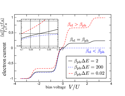
Figure 2: (Color Online) Renormalized electron current $I_{R}=I_{R1}+I_{R2}$ from Eq. (15) versus bias voltage for different phonon bath temperatures. When the boson temperature exceeds the electron temperature, the current at zero bias voltage is positive (dashed red curve), whereas the opposite is true for larger boson than electron temperatures (dotted blue curve) – compare the zoomed inset. Parameters have been chosen as $\beta_{\rm el}\Delta E\equiv\beta_{\rm el}(\upvarepsilon_{\rm B}-\upvarepsilon_{\rm A})=2$, $\beta_{\rm el}U=20$, $\mu_{L}=+V/2=-\mu_{R}$, $\mu_{U}=\mu_{D}=0$, $\Gamma_{\rm L}=\Gamma_{\rm R}=\Gamma_{\rm U}=\Gamma_{\rm D}$.

In our case, the required energy is provided by the temperature difference between the boson and fermion reservoirs.

III.2 Bosonic transfer FT

Evaluating the direct boson current between upper and lower baths requires to evaluate the full fluctuation theorem at $n_{\rm U1}=+n_{\rm ph}$ and $n_{\rm D1}=-n_{\rm ph}$ – disregarding the number of tunneled electrons at the other junctions. Formally, this corresponds to

$$P_{n_{\rm ph}} \to \frac{1}{4\pi^{2}}\int\limits_{-\pi}^{+\pi}e^{\lambda_{1}(0,0,0,0,\chi_{U},\chi_{D})t-\mathrm{i}n_{\rm ph}(\chi_{U}-\chi_{D})}d^{2}\chi\,.$$

We now consider the identities (again for similar electronic temperatures $\beta_{\rm L}=\beta_{\rm R}=\beta_{\rm el}$ only)

$$\lambda_{1}(0,0,0,0,-\chi_{U},-\chi_{D}) \stackrel{{\scriptstyle{\rm Eq.}~{}(\ref{eqn:symmetryI})}}{{=}}$$

$$\lambda_{1}\Big{(}\mathrm{i}\beta_{\rm el}(\upvarepsilon_{\rm A}-\mu_{\rm L}),\mathrm{i}\beta_{\rm el}(\upvarepsilon_{\rm A}+U-\mu_{\rm L}),$$

$$\mathrm{i}\beta_{\rm el}(\upvarepsilon_{\rm B}-\mu_{\rm R}),\mathrm{i}\beta_{\rm el}(\upvarepsilon_{\rm B}+U-\mu_{\rm R}),$$

$$\chi_{U}+\mathrm{i}\beta_{\rm U}(\upvarepsilon_{\rm B}-\upvarepsilon_{\rm A}-\mu_{\rm U}),$$

$$\chi_{D}+\mathrm{i}\beta_{\rm D}(\upvarepsilon_{\rm B}-\upvarepsilon_{\rm A}-\mu_{\rm D})\Big{)} \stackrel{{\scriptstyle{\rm Eq.}~{}(\ref{eqn:symmetryII})}}{{=}}$$

$$\lambda_{1}\Big{(}0,0,0,0,$$

$$\chi_{U}+\mathrm{i}\beta_{\rm U}(\upvarepsilon_{\rm B}-\upvarepsilon_{\rm A}-\mu_{\rm U})-\mathrm{i}\beta_{\rm el}(\upvarepsilon_{\rm B}-\upvarepsilon_{\rm A}+V),$$

$$\chi_{D}+\mathrm{i}\beta_{\rm D}(\upvarepsilon_{\rm B}-\upvarepsilon_{\rm A}-\mu_{\rm D})-\mathrm{i}\beta_{\rm el}(\upvarepsilon_{\rm B}-\upvarepsilon_{\rm A}+V)\Big{)}$$ . (36)

Finally, this implies that the bosonic transfer FT (see also e.g. jarzynski2004a ; saito2007b )

$$\frac{P_{+n_{\rm ph}}(t)}{P_{-n_{\rm ph}}(t)} \to e^{n_{\rm ph}\left[\beta_{\rm U}(\upvarepsilon_{\rm B}-\upvarepsilon_{\rm A}-\mu_{\rm U})-\beta_{\rm D}(\upvarepsilon_{\rm B}-\upvarepsilon_{\rm A}-\mu_{\rm D})\right]}$$ (37)

is not affected by the electronic transport at all, which is due to the fact that for the boson-system coupling in our model, the coupling between transferred particles and energy is tight.

III.3 Combined bosonic FT

When we do not differentiate in which of the bosonic baths phonons are counted $n_{\rm ph}=n_{\rm U1}+n_{\rm D1}$, the probability to count a given number of phonons is given by

$$P_{n_{\rm ph}} \to \frac{1}{2\pi}\int\limits_{-\pi}^{+\pi}e^{\lambda_{1}(0,0,0,0,\chi,\chi)t-\mathrm{i}n_{\rm ph}\chi}d\chi\,.$$

We now consider the identities (again for similar electronic temperatures $\beta_{\rm L}=\beta_{\rm R}=\beta_{\rm el}$ only)

$$\lambda_{1}(0,0,0,0,-\chi,-\chi) \stackrel{{\scriptstyle{\rm Eq.}~{}(\ref{eqn:symmetryI})}}{{=}}$$

$$\lambda_{1}\Big{(}\mathrm{i}\beta_{\rm el}(\upvarepsilon_{\rm A}-\mu_{\rm L}),\mathrm{i}\beta_{\rm el}(\upvarepsilon_{\rm A}+U-\mu_{\rm L}),$$

$$\mathrm{i}\beta_{\rm el}(\upvarepsilon_{\rm B}-\mu_{\rm R}),\mathrm{i}\beta_{\rm el}(\upvarepsilon_{\rm B}+U-\mu_{\rm R}),$$

$$\chi+\mathrm{i}\beta_{\rm U}(\upvarepsilon_{\rm B}-\upvarepsilon_{\rm A}-\mu_{\rm U}),$$

$$\chi+\mathrm{i}\beta_{\rm D}(\upvarepsilon_{\rm B}-\upvarepsilon_{\rm A}-\mu_{\rm D})\Big{)} \stackrel{{\scriptstyle{\rm Eq.}~{}(\ref{eqn:symmetryII})}}{{=}}$$

$$\lambda_{1}\Big{(}0,0,0,0,$$

$$\chi+\mathrm{i}\beta_{\rm U}(\upvarepsilon_{\rm B}-\upvarepsilon_{\rm A}-\mu_{\rm U})-\mathrm{i}\beta_{\rm el}(\upvarepsilon_{\rm B}-\upvarepsilon_{\rm A}+V),$$

$$\chi+\mathrm{i}\beta_{\rm D}(\upvarepsilon_{\rm B}-\upvarepsilon_{\rm A}-\mu_{\rm D})-\mathrm{i}\beta_{\rm el}(\upvarepsilon_{\rm B}-\upvarepsilon_{\rm A}+V)\Big{)} \stackrel{{\scriptstyle{\rm Eq.}~{}(\ref{eqn:symmetryIII})}}{{=}}$$

$$\lambda_{1}\Big{(}0,0,0,0,$$

$$\chi+\mathrm{i}\bar{\beta}_{\rm ph}(\upvarepsilon_{\rm B}-\upvarepsilon_{\rm A})-\mathrm{i}\beta_{\rm el}(\upvarepsilon_{\rm B}-\upvarepsilon_{\rm A}+V),$$

$$\chi+\mathrm{i}\bar{\beta}_{\rm ph}(\upvarepsilon_{\rm B}-\upvarepsilon_{\rm A})-\mathrm{i}\beta_{\rm el}(\upvarepsilon_{\rm B}-\upvarepsilon_{\rm A}+V)\Big{)} \,.$$ (39)

Finally, this implies that the combined bosonic FT

$$\frac{P_{+n_{\rm ph}}(t)}{P_{-n_{\rm ph}}(t)} \to e^{n_{\rm ph}\left[\bar{\beta}_{\rm ph}(\upvarepsilon_{\rm B}-\upvarepsilon_{\rm A})-\beta_{\rm el}(\upvarepsilon_{\rm B}-\upvarepsilon_{\rm A}+V)\right]}$$ (40)

is now affected by the electronic transport. We have also calculated the total bosonic emission rate and find qualitative agreement with the FT, see Fig. 3.

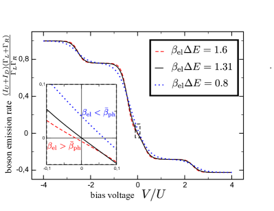
Figure 3: (Color Online) Renormalized phonon current from Eq. (15) versus bias voltage for different electron bath temperatures. At zero bias voltage (compare zoomed inset), bosons may either be created (higher electronic temperatures, dotted blue curve) or absorbed (lower electronic temperatures, dashed red curve). Parameters have been chosen as $\beta_{U}\Delta E\equiv\beta_{U}(\upvarepsilon_{\rm B}-\upvarepsilon_{\rm A})=1.0$, $\beta_{D}\Delta E=2.0$ (leading to $\bar{\beta}_{\rm ph}\Delta E\approx 1.31$ at symmetric tunneling rates $\Gamma_{\rm U}=\Gamma_{\rm D}$), $\Gamma_{\rm L}=\Gamma_{\rm R}=\Gamma_{\rm U}=\Gamma_{\rm D}$, $\beta_{D}U=20$, $\mu_{U}=\mu_{D}=0$ and $\mu_{L}=+V/2=-\mu_{R}$.

III.4 Numerical Sanity Check

We have also computed the fluctuation theorem in Eqns. (34), (37), and (40) by performing the required one- or two-dimensional integration using the dominant eigenvalue numerically. Within the boundaries of numerical accuracy, we have found complete agreement with our results (not shown). Naturally, we have also tested the independence on electronic tunneling rates and the simpler dependence on an average boson temperature.

IV Summary

We have investigated the multi-terminal fluctuation theorem for full counting statistics for a four-terminal model including bosonic and fermionic channels and Coulomb-interaction as well as phonon-assisted electron tunneling. We find that under the Born-, Markov-, and secular approximations that under the assumption of a nondegenerate system spectrum lead to the conventional rate equations, the complete FT is fully satisfied. As these rate equations satisfy local detailed balance at each terminal separately, this result was expected.

However, when not the complete information is gathered on all energy and matter fluxes, the FT may be apparently violated, formally expressed e.g. by a renormalized bias voltage. Thus, the modification of the FT may be qualitatively different from QPC back-action models but rather mimic the FT found for a Maxwell demon model. In addition, when reservoirs at different thermal states couple identically to the system, they may act as a single bath at some average thermal state – which may destroy universality of the FT (independence of the tunneling rates).

V Acknowledgments

We have profited from discussions with E. Schlottmann, R. Sanchez and G. Kießlich and also gratefully acknowledge financial support from the DFG (SCHA 1642/2-1).

References

• (1) U. Seifert, Phys. Rev. Lett. 95, 040602 (2005).
• (2) D. Andrieux and P. Gaspard, J. Chem. Phys. 121, 6167-6174 (2004).
• (3) D. Andrieux and P. Gaspard, JSTAT P01011 (2006).
• (4) D. Andrieux et al., N. J. Phys. 11, 043014 (2009).
• (5) M. Esposito, U. Harbola, and S. Mukamel, Phys. Rev. B 75, 155316 (2007).
• (6) S. Gustavsson et al., Phys. Rev. Lett. 96, 076605 (2006).
• (7) E. V. Sukhorukov et al., Nat. Phys. 3, 243 (2007).
• (8) C. Flindt et al., PNAS 106, 10116 (2009).
• (9) T. Fujisawa et al., Science 312, 1634 (2006).
• (10) Y. Utsumi et al., Phys. Rev. B 81, 125331 (2010).
• (11) J. Ren, P. Hänggi and B. Li, Phys. Rev. Lett. 104, 170601 (2010).
• (12) K. Saito and Y. Utsumi, Phys. Rev. B 78, 115429 (2008).
• (13) H. Förster and M. Büttiker, Phys. Rev. Lett. 101, 136805 (2008).
• (14) Y. Utsumi and K. Saito, Phys. Rev. B 79, 235311 (2009).
• (15) D. S. Golubev et al., Phys. Rev. B 84, 075323 (2011).
• (16) B. Küng et al., arXiv:1107.4240.
• (17) R. Sánchez et al., Phys. Rev. Lett. 104, 076801 (2010).
• (18) G. Bulnes Cuetara, M. Esposito, and P. Gaspard, Phys. Rev. B 84, 165114 (2011).
• (19) G. Schaller et al.,Phys. Rev. B 84, 085418 (2011).
• (20) M. Galperin and A. Nitzan, Phys. Rev. Lett. 95, 206802 (2005).
• (21) J. König, H. Schoeller, and G. Schön, Phys. Rev. Lett. 76, 1715 (1996).
• (22) C. Emary, Phys. Rev. B 80, 235306 (2009).
• (23) I. Garate, and I. Affleck, Phys. Rev. Lett. 106, 156803 (2011).
• (24) H.-P. Breuer and F. Petruccione, The Theory of Open Quantum Systems, (Oxford University Press, Oxford, 2002).
• (25) G. Lindblad, Commun. Math. Phys. 48, 119, (1976).
• (26) B. Rutten, M. Esposito and B. Cleuren, Phys. Rev. B 80, 235122 (2009).
• (27) M. Esposito and C. Van den Broeck, Phys. Rev. E 82, 011143 (2010).
• (28) S. A. Gurvitz and Ya. S. Prager, Phys. Rev. B 53, 15932 (1996).
• (29) G. Schaller, G. Kießlich and T. Brandes, Phys. Rev. B 80, 245107 (2009).
• (30) U. Harbola, M. Esposito and S. Mukamel, Phys. Rev. B 76, 085408 (2007).
• (31) C. Flindt, T. Novotny, and A.-P. Jauho, Phys. E 29, 411 (2005).
• (32) G. Schaller, G. Kießlich, and T. Brandes, Phys. Rev. B 81, 205305 (2010).
• (33) M. Esposito, U. Harbola, and S. Mukamel, Rev. Mod. Phys. 81, 1665 (2009).
• (34) M. Campisi, P. Hänggi, and P. Talkner, Rev. Mod. Phys. 83, 771 (2011).
• (35) G. Schaller, Phys. Rev. E 83, 031111 (2011).
• (36) R. Sánchez and M. Buttiker, Phys. Rev. B 83, 085428 (2011).
• (37) O. Entin-Wohlman, Y. Imry, and A. Aharony, Phys. Rev. B 82, 115314 (2010).
• (38) C. Jarzynski and D. K. Wójcik, Phys. Rev. Lett. 92, 230602 (2004).
• (39) K. Saito and A. Dhar, Phys. Rev. Lett. 99, 180601 (2007).