One-dimensional Particle Processes with Acceleration/Braking Asymmetry

Abstract

The slow-to-start mechanism is known to play an important role in the particular shape of the Fundamental diagram of traffic and to be associated to hysteresis effects of traffic flow. We study this question in the context of exclusion and queueing processes, by including an asymmetry between deceleration and acceleration in the formulation of these processes. For exclusions processes, this corresponds to a multi-class process with transition asymmetry between different speed levels, while for queueing processes we consider non-reversible stochastic dependency of the service rate w.r.t the number of clients. The relationship between these 2 families of models is analyzed on the ring geometry, along with their steady state properties. Spatial condensation phenomena and metastability is observed, depending on the level of the aforementioned asymmetry. In addition we provide a large deviation formulation of the fundamental diagram (FD) which includes the level of fluctuations, in the canonical ensemble when the stationary state is expressed as a product form of such generalized queues.

1 Introduction

In the study of models for traffic [1], properties of the FD, which gives a relation between the traffic flux and the density or alternatively the dependence between the speed and the flux, or the speed and the density, play an important role. In the three phases traffic theory of Kerner [2], the traffic phase diagram on highways consists of the free flow, the synchronized flow and the wide moving jam. In the free flow regime, at low density, the flux is simply proportional to the density of cars; in the congested one, at large density, massive clusters of cars are present, and the flux decreases more or less linearly with this density; in the intermediate regime, the relation between flux and density is largely of stochastic nature, due to the presence of a large amount of small clusters of cars propagating at various random speeds. It is not clear however whether in this picture these phases, and especially the synchronized flow phase, are genuine dynamical or thermodynamical phases, meaningful in some large size limit in the stationary regime, or are intricate transient features of a slowly relaxing system. In fact there is still controversy about the reality of the synchronized phase of Kerner at the moment [3].

In order to analyze properties of the FD from a statistical physics perspective, we look for a simple extension of the totally asymmetric exclusion process (TASEP) as well as the zero range process able to encode the fact that vehicles in the traffic may accelerate or brake. Some asymmetry between these two actions is empirically known to be responsible of the way spontaneous congestion occurs. This is referred as the slow-to-start mechanism, not present in the original cellular automaton of Nagel-Schreckenberg [4], but in its refined version like the velocity dependant randomized one (VDR) [5] which exhibits a first order phase transition between the fluid and the congestion phase and hysteresis phenomena [6] associated to metastable states. So a realistic stochastic model should have in particular the property that some spontaneous symmetry breaking among identical vehicles can occur, as can be seen experimentally on a ring geometry for example [7]. With such a model at hand we would like to provide a method to compute the FD and study emergence of non-trivial collective behaviors at macroscopic level.

The paper is organized as follows: in Section 2 we start by defining a simple and somewhat minimal generalization of TASEP and describe some of its basic properties. In Section 3 a family of zero-range processes is introduced which service rate depends stochastically on the state of the queue and on which there are relevant mappings of multi-speed TASEP; we determine sufficient conditions for having a product form for the invariant measure of such processes coupled in tandem. In Section 4 we provide a large deviation formulation giving the FD along with fluctuations on the ring geometry in the canonical ensemble, when the steady state has a product form. Finally, in Section 5 we analyze the jam structure of a generalized queueing process corresponding to the model introduced in Section 2. and interpret direct simulations of the multi-speed TASEP in this light.

2 Multi-speed exclusion processes

2.1 Model definition

The model we investigate is a multi-type exclusion process, generalizing the simple exclusion process on the line, introduced by Spitzer in the 70’s [8, 9], combined with some feature of the Nagel-Schreckenberg cellular automaton [4].

In the totally asymmetric version of the exclusion process [8, 9] (TASEP), particles move randomly on a 1-d lattice, always in the same direction, hopping from one site to the next one within a time interval following a Poisson distribution and conditionally that the next site is vacant. In the Nagel-Schreckenberg cellular automaton, the dynamics is in parallel: all particles update their positions at fixed time intervals, but their speeds are encoded in the number of steps that they can take. This speed can adapt stochastically, depending on the available space in front of the particle.

The model that we propose combines the braking and accelerating feature of the Nagel-Schreckenberg models, with the locality of the simple ASEP model, in which only two consecutive sites do interact at a given time. The trick is to allow each car to change stochastically its hopping rate, depending on the state of the next site. For a $2$-speed model, let $A$ denotes sites occupied by fast vehicles, $B$ sites occupied by slow ones and let $O$ denote empty sites; the model is defined by the following set of reactions, involving pairs of neighbouring sites:

$$AO \operatorname*{\longrightarrow}^{\mu_{a}}OA\qquad\text{simple move of fast vehicle}$$ (1)

$$BO \operatorname*{\longrightarrow}^{\mu_{b}}OB\qquad\text{simple move of slow vehicle}$$ (2)

$$BO \operatorname*{\longrightarrow}^{\gamma}AO\qquad\text{slow vehicle spontaneously accelerates}$$ (3)

$$A\bar{O} \operatorname*{\longrightarrow}^{\delta}B\bar{O}\qquad A\ \text{brakes behind}\ \bar{O}=A\ \text{or}\ B$$ (4)

$\mu_{a}$, $\mu_{b}$, $\gamma$ and $\delta$ denote the transition rates, each transition corresponding to a Poisson event. The dynamics is therefore purely sequential as opposed to the dynamics of the Nagel-Schreckenberg model. It encode the fact that a slow vehicle tends to accelerate when there is space ahead, while in the opposite case, corresponding to (4) it tends to slow down. The main mechanism behind congestion, namely the asymmetry between braking and acceleration is potentially present in the model when $\gamma$ is different from $\delta$. Our model is in fact similar to the model of Appert-Santen [10], in which there is a single speed, but particles have 2 states: at rest and moving with possible transitions between these 2 states.

To define fully the model, its boundary conditions have to be specified, either periodic in the ring geometry or with edges. In the latter case, additional incoming and outgoing rates have to be specified, depending on whether we want to model a traffic light a stop or simply a segment of highway for example. In this paper we will consider only the ring geometry. In the following we will refer to this specific model as the acceleration-braking totally asymmetric exclusion process (ABTASEP).

2.2 Known special cases

Let us first notice that this model contains and generalizes several sub-models which are known to be integrable with particular rates. The hopping part (1,2) of the models is just the TASEP when $\mu_{a}=\mu_{b}$, which is known to be integrable. Its generalization to include multiparticle dynamics with overtaking is the so-called Karimipour model [11, 12] which turns out to be integrable as well. Matrix Ansatz method allows in some cases, like the ASEP with open boundary conditions, to describe the stationary regime of the models, using the representations of the so-called diffusion algebras [13]. The acceleration/deceleration dynamics is equivalent to the coagulation/decoagulation models, which are known to be solvable by the empty interval method and by free fermions for particular sets of rates [14], but the whole process is presumably not integrable.

2.3 Relation to tandem queues

In some cases, the model can be exactly reformulated in terms of generalized queueing processes (or zero range processes in the statistical physics parlance), where service rates of each queue follows as well a stochastic dynamics [15]. In this previous work we however considered exclusion processes involving three consecutive sites interactions in order to maintain the homogeneity of labels in particle clusters. The mapping works only on the ring geometry, by identifying queues either with

• cars: clients are the empty sites.

• empty sites: clients are the vehicles;

In our case the mapping of type (i) is exact. In the corresponding queueing process, queues are associated either with fast or slow cars, having then service rates $\mu_{a}$ or $\mu_{b}$. Slow queues become fast at rate $\gamma$ conditionally to having at least one client, while empty fast queues become slow at rate $\delta$.

The mapping of type (ii), is more informative with respect to jam distribution, but is not possible with transitions limited to $2$-consecutive sites interactions, because in that case homogeneity is not maintained in the clusters, and additional information to the number of cars and the rate of the car leaving the queue is needed to know the service rate of the queue. For this mapping we have to resort to some approximate procedure as shall be exemplified in Section 5.

Another way to circumvent this would be to start from a a slightly different definition of our initial model, by not attaching speed labels to cars, but instead to empty sites. Let $A$ and $B$ denote empty site with respectively fast and slow speed, and $V$ denote sites occupied with a vehicle, the set of transitions reads then

$$\begin{cases}\displaystyle VA\operatorname*{\longrightarrow}^{\mu_{a}}AV\qquad\text{simple move on fast site}\\[2.84544pt] \displaystyle VB\operatorname*{\longrightarrow}^{\mu_{b}}BV\qquad\text{simple move on slow site}\\[2.84544pt] \displaystyle VA\operatorname*{\longrightarrow}^{\delta}VB\qquad\text{fast site become slow}\\[2.84544pt] \displaystyle\bar{V}B\operatorname*{\longrightarrow}^{\gamma}\bar{V}A\qquad\text{slow site become fast}\end{cases}$$ (5)

where $\bar{V}$ is an unoccupied site i.e. either $A$ or $B$. The mechanism in this model is that the empty sites visited more recently have a slower associated speed than others, leading possibly to congestion instability. The mapping to tandem queues is then straightforward: queues are associated to empty site of type $A$ or $B$ with corresponding service rate $\mu_{a}$ or $\mu_{b}$; fast queues with at least one client have a probability per unit of time $\delta$ to become a slow queue, while slow queue which are empty become fast with probability rate $\gamma$. This model generalizes directly to any speed levels. Interestingly, one see that in such a model the service rate of queues are somehow related to the lifetime of clusters. In this paper we will focus on model of Section 2.1, deferring for future work the study of model (5).

2.4 Numerical observations

Based on numerical simulations on the ring geometry, we make some observations concerning the phenomenology of the model, depending on the parameters. This is illustrated on Figure 1.

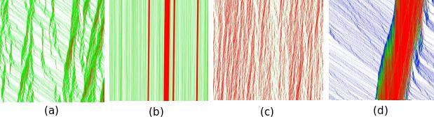
Figure 1: Space-time diagram with 2 speed levels (a)-(c) and 3 in (d). Time is going downward and particles to the right. Red, green and blue represent different speeds in increasing order. The size of the system is $3000$ except for (b) where it is $100000$. Setting are $\mu_{a}=100$, $\mu_{b}=10$, $\gamma=10$, $\delta=1$ for (a) and (b) and $\delta=10$ for (c), all with density $\rho=0.2$.

When no asymmetry between braking and accelerating is present, as in TASEP on a ring, no spontaneous large jam structure is observed. As the density $\rho$ of cars increases, one observes a smooth transition between a TASEP of fast particles for small $\rho$ to a TASEP of slow particles around $\rho\simeq 1$. Instead, when the ratio $\delta/\gamma$ is reduced, there is a proliferation of small jams. Below some threshold of this ratio, we observe a condensation phenomenon, associated to some critical value of the density: above this critical value, after a time which presumably scales as some power of $L$, one or more large jams, which absorb a finite fraction of the total number of cars may develop. If there are many of such large jams, a competition occurs, which end up possibly in the long term with one single large condensate depending on the relative value of $\gamma$ and $\mu_{b}$ and also of the size $N$ of the system. It is tempting to interpret this as a condensation mechanism at equilibrium in the canonical ensemble [16], by combining the Nagel-Paczuski [17] interpretation of competing queues with some results in a previous work [15], which in the context of tandem queues on a ring, allows this condensation mechanism to take place if the apparition of slow vehicle is a sufficiently rare event. As such, the mechanism for congestion is then understood qualitatively as follows: assume that a jam of size $s$ appears, created somewhere by a mutation $A\operatorname*{\longrightarrow}B$. Let $t(s)$ be the expected waiting time in this queue. The probability that a vehicle is still of type $A$ when it reaches the end of the queue is simply

$$p(\mu=\mu_{a})=e^{-\delta t(s)}=p_{s}.$$

Assuming that $s$ does not change much during $t(s)$, then we have

$$t(s)=s(\frac{1}{\mu_{a}}p_{s}+\frac{\mu_{a}+\gamma}{\mu_{a}(\mu_{b}+\gamma)}(1-p_{s})),$$

if we take into account the fact that the vehicle may accelerate at rate $\gamma$ before leaving the queue. Anyway, this gives $t(s)$ self-consistently and yields qualitatively that, at the beginning of the process, there is a distribution of jams with various effective service rates. As time evolves, either long-lived jams with effective service rates $\mu_{a}(\mu_{b}+\gamma)/(\mu_{a}+\gamma)$ are able to survive, then new small jams can never appear because their effective service rates are strictly larger, so in the end there is a competition between the existing jams; the largest one eventually remains alone after waiting a large amount of time. Typically this happens when $\delta\ll\mu_{b}$ and $\delta<\gamma$ (Figure 1(b)). If the situation with a single jam is not stable, then no large jam may develop at all, and only small fluctuations are to be observed. When $\delta>\gamma$ one likely observes the kind of jams seen in Figure 1(c).

Figure 2: Fundamental diagram with $\gamma=\delta$ (left) and $\gamma=10\delta$ (right) with small spontaneous rate of emission and escape of particles. Trajectories of $\Phi_{1}\stackrel{{\scriptstyle\mbox{\tiny def}}}{{=}}\sum_{i=0}^{N-1}\mu_{a}A_{i}O_{i+1}+\mu_{b}B_{i}O_{i+1}$ and $\Phi_{2}\stackrel{{\scriptstyle\mbox{\tiny def}}}{{=}}\sum_{i=0}^{N-1}\mu_{a}A_{i}+\mu_{b}B_{i}$ are displayed.

The effect of the asymmetry is also clearly observed on Figure 2, where we allow particle to enter or quit the system with some very low probability rate compared to others. The global density of cars then performs a random walk, and by looking at trajectories in the FD plane, we see hysteresis effect for $\delta<\gamma$. We have also simulated a model with $3$ speed levels, see Figure 1(d). In that case, small jams may have different speeds, depending on which type of slow car is leading. Then a cascade mechanism takes place, slow speed regions generate even slower speed clusters of cars and so on, and some kind of synchronized flow is observed.

To conclude this section, let us finally remark that Figure 1(a) is very reminiscent of coagulation-decoagulation process, which is somewhat expected from the previous discussion, since it is present in the equations. One could therefore expect the jam structure to share some properties with the directed percolation process taking place on the ring geometry.

2.5 Hydrodynamic equations and solitons

Although it is not clear whether the hydrodynamic limits is valid in our context, one can at least write down the corresponding equations on the density $\rho_{a}(x,t)$ and $\rho_{b}(x,t)$, with $x=i/N$ and $N$ large, expected in such a limit:

$$\partial_{t}\rho_{a}+v_{a}\partial_{x}(\rho_{a}\bar{\rho}) =-\delta\rho_{a}\rho+\gamma\rho_{b}\bar{\rho}$$ (6)

$$\partial_{t}\rho_{b}+v_{b}\partial_{x}(\rho_{b}\bar{\rho}) =\delta\rho_{a}\rho-\gamma\rho_{b}\bar{\rho}$$ (7)

with $\rho=\rho_{a}+\rho_{b}$ the total density of cars, $\bar{\rho}=1-\rho$ the density of empty sites and

$$v_{a,b}\stackrel{{\scriptstyle\mbox{\tiny def}}}{{=}}\lim_{N\to\infty}\frac{\mu_{a,b}^{(N)}}{N}$$

if the rates $\mu_{a,b}^{(N)}$ are allowed to be rescaled when $N$ is varied. This is an hyperbolic system of equations since the matrix

$$M=\left[\begin{matrix}v_{a}(1-2\rho_{a}-\rho_{b})&-v_{a}\rho_{a}\\ -v_{b}\rho_{b}&v_{b}(1-\rho_{a}-2\rho_{b})\end{matrix}\right]$$

has two real eigenvalues

$$\lambda^{\pm}=\frac{1}{2}\bigl{(}v_{a}+v_{b}-v_{a}(2\rho_{a}+\rho_{b})-v_{b}(\rho_{a}+2\rho_{b})\pm\sqrt{\Delta},$$

with

$$\Delta=\bigl{(}v_{a}(1-2\rho_{a}-\rho_{b})-v_{b}(1-\rho_{a}-2\rho_{b})\bigr{)}^{2}+4v_{a}v_{b}\rho_{a}\rho_{b}\ >0.$$

The method of characteristic applied to this system is however not giving much insight into it, because of the non-linear shape of the characteristics.

Figure 3:

At steady state we can nevertheless look for backward travelling waves solutions, of the form $\rho_{a,b}(x+vt)$, with $v$ the propagation velocity. Replacing $\partial_{t}$ by $v\partial_{x}$ in (6,6) and summing up the two equations one can check that the flux

$$\Phi\stackrel{{\scriptstyle\mbox{\tiny def}}}{{=}}(v_{a}\rho_{a}+v_{b}\rho_{b})\bar{\rho}+v\rho,$$ (8)

is a conserved quantity

$$\frac{d\Phi}{dx}=0.$$

This allows to express $\rho_{a}$ and $\rho_{b}$ as function of $\rho$:

$$\rho_{a}=\frac{\Phi-\rho v-v_{b}\rho\bar{\rho}}{(v_{a}-v_{b})\bar{\rho}}\qquad\text{and}\qquad\rho_{b}=\frac{\Phi-\rho v-v_{a}\rho\bar{\rho}}{(v_{b}-v_{a})\bar{\rho}}$$ (9)

After rescaling w.r.t $v_{a}$ the model has only $3$ independent parameters:

$$\eta\stackrel{{\scriptstyle\mbox{\tiny def}}}{{=}}\frac{v_{b}}{v_{a}},\qquad\kappa\stackrel{{\scriptstyle\mbox{\tiny def}}}{{=}}\frac{\delta}{\gamma},\qquad\nu\stackrel{{\scriptstyle\mbox{\tiny def}}}{{=}}\frac{\gamma}{v_{b}},$$

and we rescale as well the soliton speed $\upsilon\stackrel{{\scriptstyle\mbox{\tiny def}}}{{=}}v/v_{a}$ and the flux $\phi\stackrel{{\scriptstyle\mbox{\tiny def}}}{{=}}\Phi/v_{a}$. Replacing $\rho_{a}$ and $\rho_{b}$ with their expressions in (9), we obtain an equation relating $\partial_{x}\rho$ and $\rho$:

$$\frac{d\rho}{dx}=-C\bar{\rho}\ \frac{P(\rho)}{Q(\rho)},$$

with

$$C=\frac{\nu}{2}(1-\eta\kappa)$$

and where $P$ and $Q$ are both polynomials of degree $3$:

$$P(\rho) \stackrel{{\scriptstyle\mbox{\tiny def}}}{{=}}\bar{\rho}(\rho-\rho^{-})(\rho-\rho^{+})+\bigl{(}\frac{\nu}{2}(1-\kappa)\bar{\rho}+\kappa\nu\bigr{)}(\phi-\upsilon)$$

$$Q(\rho) \stackrel{{\scriptstyle\mbox{\tiny def}}}{{=}}\bar{\rho}^{2}(\rho-\rho_{1})+(\phi-\upsilon)\frac{\upsilon}{2\eta}$$

where

$$\rho_{1}=1+\frac{1+\eta}{\eta}\upsilon,\qquad\rho^{\pm}=\frac{1+(1-\kappa)\upsilon\pm\sqrt{\Delta}}{2(1-\eta\kappa)},$$

are the roots when $\phi=\upsilon$ with the discriminant

$$\Delta=(1-(1+\kappa)\upsilon)^{2}+4(\eta-\upsilon)\kappa\upsilon,$$

assumed to be positive. Assuming $\kappa<1$ we have $\rho^{-}\in[0,1]$ and $\rho^{+}\geq 1$ [resp. $\rho^{+}\in]\rho^{-},1]$] when $\upsilon\leq\eta$ [resp. $\upsilon\geq\eta$]. $1/C$ gives the length scale of the interface between regions of different densities. In particular if $\mu_{a,b}$ are maintained at a fixed value the interface becomes a step function when $N$ is large.

Let $\rho_{max}$ and $\rho_{min}$ the extremal values of the density. We expect a solution which decreases from $\rho_{max}$ to $\rho_{min}$ with $R(\rho)$ staying strictly positive for $\rho\in[\rho_{min},\rho_{max}]$. Since $R(\rho)$ is a single valued function of $\rho$, there must be a discontinuity, i.e. a shock to relate these two values as depicted on Figure 3. We don’t expect everything to be discontinuous at this point, in particular, as long as the shock is not at rest ($v=0$) the proportion of fast cars $u\stackrel{{\scriptstyle\mbox{\tiny def}}}{{=}}\rho_{a}/\rho$ should be continuous, since cars are slowing down at finite pace $\delta$. This means that $\rho_{min}$ and $\rho_{max}$ are not independent. Instead, letting $u^{*}$ the value of $u$ at the shock, from (9), they are both solution of ($\bar{u}^{*}\stackrel{{\scriptstyle\mbox{\tiny def}}}{{=}}1-u^{*}$)

$$(v_{a}u^{*}+v_{b}\bar{u}^{*})\rho^{2}-(v_{a}u^{*}+v_{b}\bar{u}^{*}+\upsilon)\rho+\phi=0.$$

Given that the sum and product of the two roots have to be smaller than $2$ and $1$ respectively, we deduce that $\upsilon$ and $\phi$ are both strictly smaller than $v_{a}u^{*}+v_{b}\bar{u}^{*}$. In addition the constraint $\rho_{max}\leq 1$ implies $\phi\geq\upsilon$. As a consequence, for $\rho\in[0,1[$ we have $Q(\rho)>0$, vanishing only at $\rho=1$ in the limit case $\Phi=\upsilon$. Concerning $P(\rho)$ it has then $3$ roots $\rho_{i},i\in\{1,2,3\}$ with $0<\rho_{1}<\rho_{2}<1<\rho_{3}$. To obtain a general solution, there are two free parameters, $\upsilon$ and $\rho_{min}$ and therefore $2$ constraints, associated to fixing the length of the system to one the mean density to $\rho_{0}$. These read

$$\int_{\rho_{min}}^{\rho_{max}}\frac{d\rho}{\bar{\rho}}\frac{Q(\rho)}{P(\rho)}=C\qquad\text{and}\qquad\int_{\rho_{min}}^{\rho_{max}}d\rho\frac{\rho}{\bar{\rho}}\frac{Q(\rho)}{P(\rho)}=C\rho_{0}.$$

When condensation occurs we expect to observe a full congestion ($\rho=1$) at some point. This entails from (8) that $\phi=\upsilon$, yielding in that case the equation:

$$\frac{d\rho}{dx}=C\frac{(\rho^{+}-\rho)(\rho-\rho^{-})}{\rho-\rho_{1}}.$$

and

$$\rho_{a}=\frac{\upsilon-\eta\rho}{1-\eta}\qquad\text{for}\qquad\rho<1.$$

On one hand, we should have $\rho^{+}>1$ to be able to have a point where $\rho=1$, consequently $\upsilon$ is necessarily smaller than $\eta$; on the other hand $\rho_{a}$ becomes negative when $\rho\to 1$ if $\upsilon<\eta$. As a result, there is no consistent way to obtain genuine condensation in this hydrodynamic framework.

3 Tandem queues with stochastic service rates

3.1 Definition of the process

As already mentioned in Section 2.3, in some cases, on the ring geometry, exclusion processes can be mapped onto a queueing process. These have a fixed number of queues, organized in tandem and in each queue, both the number of clients and the service rate are stochastic, the service rate being not necessarily a function of the number clients. In some case, each queue taken in isolation may not be a reversible process, with some hysteresis feature relevant to traffic. This family of models is defined more formally as follows: let ${\cal G}=({\cal N},{\cal L})$ a network of queues with dynamical (stochastic) service rates. By dynamical service rates, we mean that each single queue $i\in{\cal N}$ is represented by a vector $z_{i}(t)=(n_{i}(t),\mu_{i}(t))\in E_{i}\subset{\mathbb{N}}\times{\mathbb{R}}^{+}$. $n_{i}(t)$ is the number of clients and $\mu_{i}(t)$ is a service rate, which represents the global transition rate from $z_{i}$ to $z^{\prime}_{i}=(n_{i}-1,\mu_{i}^{\prime})\in V_{i}^{-}(z_{i})$ ($V_{i}^{-}(z)$ is the set of points in $E_{i}$ having one client less than $z$). This process is a generalization of queueing processes with stochastic service [18, 15, 14]. From the viewpoint of the statistical physics it is an extension of the zero-range process, obtained by adding internal dynamics.

Two sets of transition probability matrices $p_{i}^{\pm}(z,z^{\prime})$ and one set of transition rates $q_{i}^{0}(z,z^{\prime})$ are introduced to complete the definition of the process. When a client get served in queue $i$, there is a transition from the state of the departure queue $z_{i}$ to one of the state $z^{\prime}\in V_{i}^{-}(z)$ with a rate $\mu_{i}(t)p_{i}^{-}(z,z^{\prime})$; in the destination queue, a transition occurs from the state $z_{i+1}$ into one of state $z^{\prime}\in V_{i+1}^{+}(z)$ with probability $p_{i+1}^{+}(z,z^{\prime})$. We have the normalizations,

$$\sum_{z^{\prime}\in V_{i}^{\pm}(z)}p_{i}^{\pm}(z,z^{\prime})=1.$$ (10)

Additional internal transitions are allowed, where the service rate $\mu_{i}$ of queue $i$ changes independently of any arrival or departure. The intensities of these transitions are given by the set $q_{i}^{0}(z,z^{\prime}),\ z^{\prime}\in V_{i}^{0}(z)$ of transition rates ($V_{i}^{0}(z)$ is the set of points in $E_{i}$ having the same number of clients as $z$). The combined set of transition rates,

$$q_{i}(z,z^{\prime})\stackrel{{\scriptstyle\mbox{\tiny def}}}{{=}}\lambda p_{i}^{+}(z,z^{\prime})\leavevmode\hbox{\rm\small 1\kern-3.15005pt\normalsize 1}_{\{z^{\prime}\in V_{i}^{+}(z)\}}+\mu(z)p_{i}^{-}(z,z^{\prime})\leavevmode\hbox{\rm\small 1\kern-3.15005pt\normalsize 1}_{\{z^{\prime}\in V_{i}^{-}(z)\}}+q_{i}^{0}(z,z^{\prime})\leavevmode\hbox{\rm\small 1\kern-3.15005pt\normalsize 1}_{\{z^{\prime}\in V_{i}^{0}(z)\}},$$

defines for each $i\in{\cal N}$ a continuous time Markov process representing the dynamics of one queue taken in isolation with arrival rate $\lambda$. The joint process is then entirely specified by the state graph of the single queue which set of nodes $\{(n,\mu)\}$ is a subset of ${\mathbb{N}}\times{\mathbb{R}}_{+}$, and in which each transition is represented by an oriented edge (see e.g. Figures 4 and 5).

3.2 Product form of clusters at steady-state

In the stationary regime, the invariant measure of a network of reversible queues is known to factorize into a product form in general [19], which allows to compute many equilibrium quantities explicitly. With a dynamical rate it is interesting to check for such properties and in this section we study the conditions under which the stationary state has a product form. For simplicity we restrict the analysis to the case where $\cal G$ corresponds to a tandem of $N$ queues where the clients leave queue $i$ to enter in queue $(i+1)\mod(N)$, for any $i=0,\ldots,N-1$. We can establish the following sufficient conditions:

Theorem 3.1.

Let $\pi_{i}^{\lambda}$ denotes the steady state probability corresponding to queue $i$ taken in isolation and fed with a Poisson process with rate $\lambda$. If the following partial balance equations are satisfied (see Figure 4),

$$\sum_{z\in V_{i}^{+}(z_{i})}\mu(z)p_{i}^{-}(z,z_{i})\pi_{i}^{\lambda}(z)\ =\lambda\pi_{i}^{\lambda}(z_{i}),$$ (11)

$$\mu(z_{i})\pi_{i}^{\lambda}(z_{i})\ +\sum_{z\in V_{i}^{0}(z_{i})}q_{i}^{0}(z_{i},z)\pi_{i}^{\lambda}(z_{i}) =$$

$$\sum_{z\in V_{i}^{-}(z_{i})}\lambda p_{i}^{+}(z,z_{i})\pi_{i}^{\lambda}(z) +\sum_{z\in V_{i}^{0}(z_{i})}q_{i}^{0}(z,z_{i})\pi_{i}^{\lambda}(z),$$ (12)

then the joint probability measure of the network has the following product form at steady state:

$$P(S=\{z_{i},i\in{\cal N}\})=\frac{\prod_{i\in{\cal N}}\pi_{i}^{\lambda}(z_{i})}{P(\sum_{i}n_{i}=N)}$$ (13)

Proof.

Using (10), the global balance equations reads

$$\sum_{i\in{\cal N}}\Biggl{[}\sum_{\begin{subarray}{c}z^{\prime}\in V_{i}^{+}(z_{i})\\ z^{\prime\prime}\in V_{i+1}^{-}(z_{i+1})\end{subarray}}\mu(z^{\prime})p_{i}^{-}(z^{\prime},z_{i}) p_{i+1}^{+}(z^{\prime\prime},z_{i+1})\frac{\pi_{i}^{\lambda}(z^{\prime})\pi_{i+1}^{\lambda}(z^{\prime\prime})}{\pi_{i}^{\lambda}(z_{i})\pi_{i+1}^{\lambda}(z_{i+1})}$$

$$+\sum_{z\in V_{i}^{0}(z_{i})}q_{i}^{0}(z,z_{i})\frac{\pi_{i}^{\lambda}(z)}{\pi_{i}^{\lambda}(z_{i})}\Biggr{]}P(S=\{z_{i}\})$$

$$=\ \sum_{i\in{\cal N}}\Bigl{[}\mu(z_{i})+\sum_{z\in V_{i}^{0}(z_{i})}q_{i}^{0}(z_{i},z)\Bigr{]}P(S=\{z_{i}\})$$

To find a sufficient condition select term $i$ in the first term of the left hand side and terms $i+1$ otherwise in the preceding equation, yielding $\forall i\in{\cal N}$,

$$\sum_{\begin{subarray}{c}z^{\prime}\in V_{i}^{+}(z_{i})\\ z^{\prime\prime}\in V_{i+1}^{-}(z_{i+1})\end{subarray}}\mu(z^{\prime})p_{i}^{-}(z^{\prime},z_{i})p_{i+1}^{+}(z^{\prime\prime},z_{i+1}) \pi_{i}^{\lambda}(z^{\prime})\pi_{i+1}^{\lambda}(z^{\prime\prime})+$$

$$\sum_{z\in V_{i+1}^{0}(z_{i+1})}q_{i+1}^{0}(z,z_{i+1})\pi_{i}^{\lambda}(z_{i})\pi_{i+1}^{\lambda}(z)$$

$$=\mu(z_{i+1})\pi_{i}^{\lambda}(z_{i})\pi_{i+1}^{\lambda}(z_{i+1}) +\sum_{z\in V_{i+1}^{0}(z_{i+1})}q_{i+1}^{0}(z_{i+1},z)\pi_{i}^{\lambda}(z_{i})\pi_{i+1}^{\lambda}(z_{i+1}).$$

After multiplying this last equation by $\lambda$, this sufficient condition rewrites

$$\Bigl{(}\sum_{z^{\prime}\in V_{i}^{+}(z_{i})}\mu(z^{\prime})p_{i}^{-}(z^{\prime},z_{i})\pi_{i}^{\lambda}(z^{\prime})\Bigr{)} \Bigl{(}\lambda\sum_{z^{\prime\prime}\in V_{i+1}^{-}(z_{i+1})}p_{i+1}^{+}(z^{\prime\prime},z_{i+1})\pi_{i+1}^{\lambda}(z^{\prime\prime})\Bigr{)}$$

$$=\lambda\pi_{i}^{\lambda}(z_{i})\times$$

$$\Bigl{(}\mu(z_{i+1})\pi_{i+1}^{\lambda}(z_{i+1})+\sum_{z\in V_{i+1}^{0}(z_{i+1})} q_{i+1}^{0}(z_{i+1},z)\pi_{i+1}^{\lambda}(z_{i+1})-q_{i+1}^{0}(z,z_{i+1})\pi_{i+1}^{\lambda}(z)\Bigr{)},$$

which is satisfied $\forall i\in{\cal N}$ under the two sets of sufficient conditions (11) and (12).  

Note that reversible processes are special cases of processes obeying (11,12) and, in this respect, our result is an adaptation to our context of the general results of Kelly concerning product forms in queueing networks [19]. The next obvious question is then whether there exists any such process which is non-reversible.

3.3 Examples

Figure 4: (a) Partial balance condition corresponding to (11) and (12). (b) Example of a non-reversible single queue process obeying to this condition.

Let us give two examples of non-reversible queues yielding a product form. The isolated-queue state-graph corresponding to the first one is sketched in Figure 4(b). Using the labelling $(0)=(0,\mu_{0})$, $(1)=(1,\mu_{1})$, $(2)=(1,\mu_{2})$, $(3)=(2,\mu_{4})$ and $(i)=(n-2,\mu_{i})$ for $i\geq 4$ for the different states of the isolated queue, these partial balance conditions written for the nodes $(i),i<4$ yield four independent relations out of six, between the single queues steady states probabilities $\pi_{i}$:

$$\lambda\pi_{0}=\mu_{1}\pi_{1}+\mu_{2}\pi_{2}, \qquad\lambda\pi_{1}=\mu_{3}p_{31}\pi_{3},$$

$$q_{21}\pi_{2}=(q_{12}+\mu_{1})\pi_{1}, \qquad\lambda\pi_{2}=\mu_{3}p_{32}\pi_{3},$$

which are actually compatible iff:

$$\frac{p_{32}}{p_{31}}=\frac{q_{12}+\mu_{1}}{q_{21}}.$$

Letting $p\stackrel{{\scriptstyle\mbox{\tiny def}}}{{=}}p_{31}=1-p_{32}$, this corresponds to

$$p=\frac{q_{21}}{\mu_{1}+q_{12}+q_{21}}.$$

For $i\geq 4$, detail balance holds anyway. When this hold the joint measure of the tandem queue takes the product form (13) whereas this example is by construction never reversible (transitions $0\to 1$ is absent), with the single queue invariant measure simply reading

$$\pi_{1} =\frac{\lambda q_{12}}{\mu_{1}\mu_{2}+q_{12}\mu_{2}+q_{21}\mu_{1}}\pi_{0},\qquad\pi_{2}=\frac{\lambda(\mu_{1}+q_{21})}{\mu_{1}\mu_{2}+q_{12}\mu_{2}+q_{21}\mu_{1}}\pi_{0},$$

$$\pi_{3} =\frac{\lambda^{2}(\mu_{1}+q_{12}+q_{21})}{\mu_{3}(\mu_{1}\mu_{2}+q_{12}\mu_{2}+q_{21}\mu_{1})}\pi_{0},\qquad\pi_{n\geq 4}=\biggl{[}\prod_{i=4}^{n}\frac{\lambda}{\mu_{i}}\biggr{]}\frac{\lambda q_{12}}{\mu_{1}\mu_{2}+q_{12}\mu_{2}+q_{21}\mu_{1}}\pi_{0},$$

where $\pi_{0}$ is set upon normalization.

Figure 5: Composite traffic tandem queue process. Equivalence with exclusion process (left). Corresponding process in isolation, $p=\rho_{1}^{n-1}\frac{\rho_{1}-\rho_{2}}{\rho_{1}^{n}-\rho_{2}^{n}}$ (right)

Our second example is depicted in Figure 5. It represents an exclusion process on a ring, where particles, to hop to the next site have to follow a cascading process. For sake of simplicity let us limit ourselves to a two stage cascade, where empty site are of two different types: either blocking type $B$ and non-blocking type $A$. The transition rules then read:

$$VA \operatorname*{\longrightarrow}^{\mu_{1}}BV\qquad\text{vehicle hopping }$$ (14)

$$VB \operatorname*{\longrightarrow}^{\mu_{2}}VA\qquad\text{blocking site becomes non-blocking}$$ (15)

$$AB \operatorname*{\longrightarrow}^{\mu_{2}}AA\qquad\text{blocking site becomes non-blocking}$$ (16)

This model is mapped on a composite queueing process as follows: cars represent composite queues, with client arriving in the type $B$ (first stage of the composite queue) and able to jump to the second stage in type $A$ when they reach the server of the queue, i.e. when the left neighbor is of type $A$. The whole tandem of queues has a product form since each single queue taken in isolation is reversible. Considering then the queue depicted on Figure 5(b) as an effective equivalent to the composite one, it is clearly non-reversible. Nevertheless the partial balance sufficient condition for having a product form are fulfilled. Indeed in the example of the figure the isolated effective queue has for invariant measure

$$\pi(n,\tilde{\mu}=\frac{\mu_{1}\mu_{2}}{\mu_{1}+\mu_{2}}) =(1-\rho_{1})(1-\rho_{2})\rho_{1}^{n},$$

$$\pi(n,\tilde{\mu}=\mu_{1}) =(1-\rho_{1})(1-\rho_{2})\frac{\rho_{1}^{n}-\rho_{2}^{n}}{\rho_{1}-\rho_{2}},$$

with $\rho_{1,2}=\lambda/\mu_{1,2}$. Computing the fluxes yields then the desired partial balance conditions. It seems that this procedure of replacing composite of reversible queues with effective one yield automatically non-reversible queues fulfilling the partial balance conditions.

The analysis of the fundamental diagram follows then almost straightforwardly when such product form is present, although some non-trivial feature are also expected depending on the value of the spectral gap between the steady-state and the first excited state.

4 Fundamental diagram for product form distributions

4.1 Large deviation formulation

In practice, points plotted in experimental fd studies are obtained by averaging data from static loop detectors over a few minutes (see e.g. [2]). This is difficult to compute from our queue-based model, for which a space average is much easier to obtain. The equivalence between time and space averaging is not an obvious assumption [6], but since jams are moving, space and time correlations are combined in some way [17] and we consider this assumption to be quite safe. In what follows, we will therefore compute the fd by considering the conditional probability measure $P(\phi|d)$ for a closed system, where $d$ represents the spatial density of cars and $\phi$ the normalized flux:

$$\begin{cases}\displaystyle d=\frac{N}{N+L},\\[5.69046pt] \displaystyle\phi=\frac{\Phi}{N+L},\end{cases}\ \text{with}\ \begin{cases}L&\text{number of queues}\\ \displaystyle N=\sum_{i=1}^{L}n_{i}&\text{number of vehicles}\\[5.69046pt] \displaystyle\Phi=\sum_{i=1}^{L}\mu_{i}\leavevmode\hbox{\rm\small 1\kern-3.15005pt\normalsize 1}_{\{n_{i}>0\}}&\text{integrated flow}\end{cases}$$

The numbers $N$ of vehicles and $L$ of queues are fixed, meaning in the statistical physics parlance, that we are working with the canonical ensemble. If we assume that we are in the conditions of having a product form presented in the preceding section, for the stationary distribution with individual probabilities $\pi^{\lambda}(n,\mu)$ associated to each queue taken in isolation then, taking into account the constraints yields the following form of the joint probability measure:

$$P(\{n_{i},\mu_{i}\})=\frac{\delta\bigl{(}\textstyle N-\sum_{i=1}^{L}n_{i}\bigr{)}}{Z_{L}[N]}\prod_{i=1}^{L}\pi^{\lambda}(n_{i},\mu_{i}),$$

with the canonical partition function

$$Z_{L}[N]\stackrel{{\scriptstyle\mbox{\tiny def}}}{{=}}{\sum_{\{n_{i},\mu_{i}\}}\delta\bigl{(}\textstyle N-\sum_{i=1}^{L}n_{i}\bigr{)}}\prod_{i=1}^{L}\pi^{\lambda}(n_{i},\mu_{i}),$$

where $\delta$ denotes now the usual Dirac function. When $\phi$ is interpreted as a continuous variable, the properly normalized density-flow conditional probability distribution takes the form

$$P(\phi|d)=\frac{L}{1-d}\frac{Z_{L}\bigl{[}L\frac{d}{1-d},L\frac{\phi}{1-d}\bigr{]}}{Z_{L}\bigl{[}L\frac{d}{1-d}\bigr{]}},$$ (17)

with

$$Z_{L}[N,\Phi]\stackrel{{\scriptstyle\mbox{\tiny def}}}{{=}}{\sum_{\{n_{i},\mu_{i}\}}\textstyle\delta\bigl{(}N-\sum_{i=1}^{L}n_{i}\bigr{)}\delta\bigl{(}\Phi-\sum_{i=1}^{L}\mu_{i}\leavevmode\hbox{\rm\small 1\kern-3.15005pt\normalsize 1}_{\{n_{i}>0\}}\bigr{)}}\prod_{i=1}^{L}\pi^{\lambda}(n_{i},\mu_{i}),$$ (18)

Note (by simple inspection, see e.g. [19]) that $P(\phi|d)$ is independent of $\lambda$. $Z_{L}[N]$ and $Z_{L}[N,\Phi]$ represent respectively the probability of having $N$ vehicles and the joint probability for having at the same time $N$ vehicles and a flux $\Phi$, under the unconstrained product form. Under this product form, on general ground, we expect $d$ and $\phi$ to satisfy a large deviation principle (see [20] for a recent review connecting large deviations to statistical physics), i.e. that there exist two rate functions $I(d)$ and $J(d,\phi)$ such that for large $L$

$$Z_{L}(N)\asymp e^{-LI(d)},$$

$$Z_{L}[N,\Phi]\asymp e^{-LJ(d,\phi)},$$

such that we expect a the large deviation version of the fundamental diagram of the form

$$P(\phi|d)\asymp e^{-LK(\phi|d)}.$$ (19)

with

$$K(\phi|d)\stackrel{{\scriptstyle\mbox{\tiny def}}}{{=}}J(d,\phi)-I(d).$$

When there is one single constraint like for $Z_{L}(N)$, the large deviation expression can be obtained by saddle point techniques like in [16, 21]. For more than one constraint it seems easier to work variationally. Consider $L_{n,\mu}$ the number of queues having $n$ clients and service rate $\mu$. Assuming $\mu$ runs over discrete values, the partition function (18) can be recast in:

$$Z_{L}(N,\Phi) =\sum_{\{L_{n,\mu}\}}\frac{L!}{\prod_{n,\mu}L_{n,\mu}!}\prod_{n,\mu}\pi^{\lambda}(n,\mu)^{L_{n,\mu}}$$

$$\times\delta\bigl{(}L-\sum_{n,\mu}L_{n,\mu}\bigr{)}\delta\bigl{(}N-\sum_{n,\mu}nL_{n,\mu}\bigr{)}\delta\bigl{(}\Phi-\sum_{n>0,\mu}\mu L_{n,\mu}\bigr{)}$$ (20)

As can be seen explicitly in the following, when there is no condensation, i.e. no heavy tail in the $L(n,\mu)$ distribution, we are in the condition of the Sanov theorem [20] to get an asymptotic expression of the partition function. Namely,

$$Z_{L}(N,\Phi)\asymp\sum_{\{y(n,\mu)\}}\exp\Bigl{(}-L{\cal F}[y]\Bigr{)}\delta\bigl{(}C_{1}[y]\bigr{)}\delta\bigl{(}C_{2}[y]\bigr{)}\delta\bigl{(}C_{3}[y]\bigr{)},$$ (21)

with

$$y(n,\mu)\stackrel{{\scriptstyle\mbox{\tiny def}}}{{=}}\frac{L_{n,\mu}}{L}$$

the fraction of queues having $n$ clients and service rate $\mu$, ${\cal F}$ the large deviation functional and $C_{1,2,3}[y]$ the constraints:

$$C_{1}[y] =\sum_{n,\mu}y(n,\mu)-1,$$

$$C_{2}[y] =\sum_{n,\mu}ny(n,\mu)-\frac{d}{1-d},$$

$$C_{3}[y] =\sum_{n>0,\mu}\mu y(n,\mu)-\frac{\phi}{1-d}.$$

This is obtained explicitly by making use of the Stirling formula in (20), keeping only the leading terms to get:

$${\cal F}(y)=\sum_{n,\mu}y(n,\mu)\log\frac{y(n,\mu)}{\pi^{\lambda}(n,\mu)}.$$ (22)

The rate functions are then obtained using the contraction principle [20]:

$$I(d) =\inf_{\{y:C_{1}[y]=0,C_{2}[y]=0\}}{\cal F}[y]$$

$$J(d,\phi) =\inf_{\{y:C_{1}[y]=0,C_{2}[y]=0,C_{3}[y]=0\}}{\cal F}[y]$$

which apply here simply because $\cal F$ is convex and the constraints are linear. The variational principle consists in to look for a distribution $y$ minimizing the mutual information with the product form while satisfying the constraints; in this sense it is equivalent to the standard mean field approximation. A simple generalization would then amount to consider, in case where the product form is not valid, the 2-server problem to build a joint-law based on pairs $\pi^{\lambda}(n_{1},\mu_{1};n_{2},\mu_{2})$ of nearest neighbor dependencies and to use the Bethe approximation.

Let us introduce the moment and cumulant generating function $g$ and $h$ associated to $\pi^{\lambda}$,

$$g(s,t)\stackrel{{\scriptstyle\mbox{\tiny def}}}{{=}}\sum_{n=0,\mu}^{\infty}\pi^{\lambda}(n,\mu)e^{sn+t\mu}\qquad\text{and}\qquad h(s,t)\stackrel{{\scriptstyle\mbox{\tiny def}}}{{=}}\log[g(s,t)],$$

where it is assumed by convention that the rate $\mu$ is zero in absence of client. The stationary point then reads

$$y(n,\mu)=\frac{\pi^{\lambda}(n,\mu)e^{n\lambda_{n}+\mu\lambda_{\mu}}}{g(\lambda_{n},\lambda_{\mu})},$$ (23)

with the Lagrange multipliers $\lambda_{n}$ and $\lambda_{\mu}$ associated to constraints $C_{2}$ and $C_{3}$, are implicitly given by

$$\begin{cases}\displaystyle\frac{\partial h}{\partial s}\bigl{(}\lambda_{n}(d,\phi),\lambda_{\mu}(d,\phi)\bigr{)}=\frac{d}{1-d},\\[8.5359pt] \displaystyle\frac{\partial h}{\partial t}\bigl{(}\lambda_{n}(d,\phi),\lambda_{\mu}(d,\phi)\bigr{)}=\frac{\phi}{1-d}.\end{cases}$$ (24)

Inserting the variational solution (23) into $\cal F$ leads to the resulting expression of the rate function as the Legendre transform of $h$

$$J(d,\phi)=\frac{d}{1-d}\lambda_{n}(d,\phi)+\frac{\phi}{1-d}\lambda_{\mu}(d,\phi)-h\bigl{(}\lambda_{n}(d,\phi),\lambda_{\mu}(d,\phi)\bigr{)}$$

which could actually be obtained directly from Cramer’s theorem because $\{(n_{i},\mu_{i})\}$ are iid [20]. Concerning the other rate $I(d)$ function, if $\lambda_{n}^{\prime}(d)$ is associated to the first constraint, while $\lambda_{\mu}$ is set to zero we get

$$I(d)=\frac{d}{1-d}\lambda_{n}^{\prime}(d)-h\bigl{(}\lambda_{n}^{\prime}(d),0\bigr{)}$$

in term of the cumulant generating function $h$, which completes the determination of the large deviation FD (19).

4.2 Gaussian fluctuations around the fundamental diagram

The deterministic part of the fundamental diagram is then obtained for $\phi(d)$ such that,

$$\frac{\partial J(d,\phi)}{\partial\phi}\Big{|}_{d,\phi(d)}=\frac{\lambda_{\mu}(d,\phi(d))}{1-d}=0.$$ (25)

When considering small fluctuations rather than large deviations, we recover a central limit theorem version of the fundamental diagram. In that case, replacing in (21) $\cal F$ with its quadratic approximation around some stationary point value $y^{*}$ of $y$ yields the following expression for the partitions functions:

$$Z_{L}(N) \simeq\frac{\exp\bigl{(}-LI(d)\bigr{)}\bigr{)}}{\sqrt{2\pi Lh_{ss}({\lambda^{\prime}}_{n},0)}}$$ (26)

$$Z_{L}(N,\Phi) \simeq\frac{\exp\bigr{(}-LJ(d,\phi)\bigl{)}}{\sqrt{(2\pi L)^{2}\det\bigl{(}H^{\star}(\lambda_{n},\lambda_{\mu})\bigr{)}}}$$ (27)

with $(\lambda_{n},\lambda_{\mu})$ and ${\lambda^{\prime}}_{n}$ solving the constraints (24) for a given value of $d$ and $\phi$ and denoting

$$H^{\star}(s,t)\stackrel{{\scriptstyle\mbox{\tiny def}}}{{=}}\left[\begin{matrix}h_{ss}&h_{st}\\ h_{ts}&h_{tt}\end{matrix}\right],$$ (28)

with the use of shorthand notations for the derivatives, to represent the covariant matrix between the charges of the queues and the flux. This matrix is actually the Hessian in the dual representation, associated to the Legendre transform of the free energy (see Appendix A for details). We obtain for the large deviation FD the expression

$$P(\phi|d)=\sqrt{\frac{L}{2\pi(1-d)^{2}}\frac{h_{ss}(\lambda_{n}^{\prime},0)}{\det\bigl{(}H^{\star}(\lambda_{n},\lambda_{\mu})\bigr{)}}}\exp\bigr{(}-LK(\phi|d)).$$

The Taylor expansion at second order in $\phi-\phi(d)$ at fixed density is performed, using (25) so that

$$J\bigl{(}d,\phi(d)\bigr{)}=I(d).$$

and

$$\frac{\partial^{2}J(d,\phi)}{\partial\phi^{2}}|_{d,\phi(d)}=\frac{1}{1-d}\frac{\partial\lambda_{\mu}(d,\phi)}{\partial\phi}|_{d,\phi(d)}=\frac{1}{(1-d)^{2}}\frac{h_{ss}(\lambda_{n},\lambda_{\mu})}{\det(H^{\star}(\lambda_{n},\lambda_{\mu}))}.$$

The last equality is obtained by remarking that from the constraints (24) we have

$$\frac{\partial\lambda_{n}}{\partial\phi}h_{ss}+\frac{\partial\lambda_{\mu}}{\partial\phi}h_{st} =0$$

$$\frac{\partial\lambda_{n}}{\partial\phi}h_{st}+\frac{\partial\lambda_{\mu}}{\partial\phi}h_{tt} =\frac{1}{1-d},$$

from which $\partial\lambda_{\mu}/\partial\phi$ can be eliminated to yield the result. Therefore,

$$K(\phi|d)=\frac{\bigl{(}\phi-\phi(d)\bigr{)}^{2}}{2(1-d)^{2}}\frac{h_{ss}}{\det(H^{\star}(\lambda_{n},\lambda_{\mu})}+o\bigl{(}\phi-\phi(d)\bigr{)}^{2}.$$

giving the Gaussian fluctuations of the FD. The variance as a function of the density then reads

$$\operatorname{Var}(\phi|d)=\frac{(1-d)^{2}}{L}\frac{\det(H^{\star}(\lambda_{n}(d),0)}{h_{ss}(\lambda_{n}(d),0)}=\frac{(1-d)^{2}}{L}\bigl{(}{H^{\star-1}}_{tt}\bigr{)}^{-1}.$$ (29)

4.3 Special case: the TASEP

Let us apply this formula first to the simple M/M/1 file corresponding to one single speed level ($\mu_{a}=\mu_{b}=\mu$), i.e. a TASEP process. The rate of arrival $\lambda$ is set by convenience to $\lambda=d\mu$. The cumulant-generating function then reads

$$h(s,t)=\log(1-d)+\log\frac{1+de^{-s}(e^{-tv}-1)}{1-de^{-s}}.$$

Therefore we have

$$\det(H^{\star}(0,0))=\left|\begin{matrix}\displaystyle\frac{d}{(1-d)^{2}}&d\mu\\[5.69046pt] \displaystyle d\mu&d(1-d)\mu^{2}\end{matrix}\right|=\frac{d^{3}}{1-d}\mu^{2},$$

while $\mathbb{E}[\phi|d]=\mu d(1-d)$. Equation (29) yields

$$\operatorname{Var}_{\text{var}}(\phi|d)=\frac{1-d}{L}d^{2}(1-d)^{2}\mu^{2}.$$ (30)

The direct result, in the grand canonical ensemble, with expectation constraint on the density is given by

$$\operatorname{Var}_{\text{GC}}(\phi|d)=\frac{1-d}{L}h_{tt}=\frac{1-d}{L}d(1-d).$$

Actually, the TASEP computation on the ring geometry can be done directly as

$$\frac{1}{\mu^{2}}\text{Var}(\phi|d) =\text{Var}\Bigl{(}\frac{1}{N+L}\sum_{i=1}^{N+L}\tau_{i}\bar{\tau}_{i+1}\Bigr{)}$$

$$=\frac{(L+N)(L+N-3)}{(L+N)^{2}}\mathbb{E}(\tau_{i}\bar{\tau}_{i+1}\tau_{j}\bar{\tau}_{j+1})$$

$$+\frac{1}{L+N}\mathbb{E}(\tau_{i}\bar{\tau}_{i+1})-\frac{1}{(L+N)^{2}}\Bigl{(}\mathbb{E}(\tau_{i}\bar{\tau}_{i+1})\Bigr{)}^{2},$$

with $\bar{\tau}_{i}=1-\tau_{i}\in\{0,1\}$, $\tau_{N+L+1}=\tau_{1}$ and $\forall(i,j)$ s.t. $|i-j|\geq 2$. The expressions above are computed as to give

$$\mathbb{E}(\tau_{i}\bar{\tau}_{i+1})=\frac{NL}{(L+N)(L+N-1)}=d(1-d)(1+\frac{1}{L+N})+o\bigl{(}\frac{1}{L+N}\bigr{)}$$

and

$$\mathbb{E}(\tau_{i}\bar{\tau}_{i+1}\tau_{j}\bar{\tau}_{j+1}) =\frac{N(N-1)L(L-1)}{(L+N)(L+N-1)(L+N-2)(L+N-3)}$$

$$=d^{2}(1-d)^{2}(1+\frac{6}{L+N})-\frac{1}{L+N}d(1-d)+o\bigl{(}\frac{1}{L+N}\bigr{)},$$

which finally yields (30).

5 Queues with two-state service rates

Among the possible mappings discussed in Section 2.3, taking empty sites as queues should give more information on the jam structure, i.e. presumably on the long range correlations of the model associated to cluster formations, than the mapping of type (i). Unfortunately, the mapping of type (ii) is not exact in this case. Nevertheless, let us try to define a queueing process able to capture these correlations at least qualitatively.

The first step that we take in this direction is to understand the dynamics and steady state regime of a single cluster of vehicles of size $n_{t}$, assuming that vehicles of type $A$ [resp. $B$] join the queue with rate $\lambda_{a}$ [resp. $\lambda_{b}$], while they leaves the queue with rate $\mu_{a}$ [resp. $\mu_{b}$]. Let $\lambda\stackrel{{\scriptstyle\mbox{\tiny def}}}{{=}}\lambda_{a}+\lambda_{b}$ represent the intensity of the incoming process. In the bulk of the queue, accordingly to the transitions rules defined in Section 2.1, only deceleration is possible, with rate $\delta$.

5.1 Speed profile inside a single cluster

To study the speed profile, i.e. the speed labels of particle depending on their position inside a cluster, let us encode a given cluster configuration as a binary sequence $\{(A_{0},\ldots,A_{n-1}\}$, with $A_{i}=1-B_{i},\in\{0,1\}$, corresponding to either a fast or a slow vehicle. $n$ represents the size of the queue, the front vehicle has index $n-1$ while index $0$ corresponds to the last entered one. Let us remark first that the front end of the queue is a moving interface, which next $n$ moves are completely conditioned by the present state of the sequence. Let us forget about this interface for the moment and consider the distribution of the infinite sequence $\{(A_{1},A_{2},A_{3},\ldots\}$. The joint law has not a product form, because the whole sequence is shifted by one unit ($A_{i}\operatorname*{\longrightarrow}A_{i+1}$) at instants of arrival, which causes dependencies between neighbors. Nevertheless, the structure of dependency is quite simple, for example single site marginals are determined in close form. Let $p_{i}(t)=P_{t}(A_{i}=1)$, we have

$$\frac{dp_{i}}{dt} =\lambda(p_{i-1}-p_{i})-\delta p_{i},\qquad\forall i>1$$

$$\frac{dp_{1}}{dt} =\lambda_{a}(1-p_{1})-(\lambda_{b}+\delta)p_{1},$$

with $\lambda\stackrel{{\scriptstyle\mbox{\tiny def}}}{{=}}\lambda_{a}+\lambda_{b}$. The generating function

$$\phi_{t}(z)\stackrel{{\scriptstyle\mbox{\tiny def}}}{{=}}\sum_{i=0}^{\infty}p_{i+1}(t)z^{i},$$

satisfies

$$\frac{d\phi_{t}(z)}{dt}=\bigl{(}\lambda z-(\lambda+\delta)\bigr{)}\phi_{t}(z)+\lambda_{a},$$

with solution

$$\phi_{t}(z)=\frac{\lambda_{a}+\phi_{0}(z)e^{-(\lambda+\delta-\lambda z)t}}{\lambda+\delta-\lambda z}.$$

Correlations between nearest neighbors, $q_{i}(t)\stackrel{{\scriptstyle\mbox{\tiny def}}}{{=}}P_{t}(A_{i}=1,A_{i+1}=1)$ satisfy a similar closed form equation:

$$\frac{dq_{i}}{dt} =\lambda(q_{i-1}-q_{i})-2\delta q_{i},\qquad\forall i\geq 1$$

$$\frac{dq_{1}}{dt} =\lambda_{a}p_{1}(t)-(\lambda+2\delta)q_{1},$$

with

$$p_{1}(t)=\frac{\lambda_{a}+p_{1}(0)e^{-(\lambda+\delta)t}}{\lambda+\delta},$$

which generating function

$$\psi_{t}(z)\stackrel{{\scriptstyle\mbox{\tiny def}}}{{=}}\sum_{i=0}^{\infty}q_{i}(t)z^{i},$$

satisfies

$$\frac{d\psi_{t}(z)}{dt}=\bigl{(}\lambda z-(\lambda+2\delta)\bigr{)}\psi_{t}(z)+\lambda_{a}p_{1}(t),$$

having for solution:

$$\psi_{t}(z) =\frac{\lambda_{a}^{2}}{(\lambda+\delta)(\lambda+2\delta-\lambda z)}$$

$$+\bigl{(}\psi_{0}(z)-\frac{\lambda_{a}^{2}}{(\lambda+\delta)(\lambda+2\delta-\lambda z)}+\frac{\lambda^{2}}{(\lambda+\delta)\lambda z}p_{1}(0)(1-e^{-\lambda zt})\bigr{)}e^{-(\lambda+2\delta-\lambda z)t}.$$

At steady state we see that

$$p_{i}^{\infty}=\frac{\lambda_{a}}{\lambda}\Bigl{(}\frac{\lambda}{\lambda+\delta}\Bigr{)}^{i}\qquad\text{and}\qquad q_{i}^{\infty}=\frac{\lambda_{a}^{2}}{\lambda(\lambda+\delta)}\Bigl{(}\frac{\lambda}{\lambda+2\delta}\Bigr{)}^{i},$$

indicating a significant level of correlations when $\delta/\lambda$ is $O(1)$.

Figure 6: (a) State flow diagram of a queue with stochastic service rate. (b) Details of the transition rates.

5.2 Joined effective process $\bigl{(}n(t),\mu(t)\bigr{)}$

Since the front end interface of the cluster has no causal effect on the rest of the queue, except for the front vehicle which may accelerate with rate $\gamma$, we can consider the dynamics of the sequence independently of the motion of the front interface. Making the additional assumption of independence of the local speed labels in the bulk is rather crude regarding the results of the previous section, but nevertheless we look for a qualitative comparison. To this end let us write a master equation of the joint process $(n(t),\mu(t))$, i.e. the equation governing the evolution of the joint probability $P_{t}(n,\tau)=P(n(t)=n,\mu=\mu_{a}\tau+\mu_{b}\bar{\tau})$, the joint probability that the queue has $n$ clients and its front car is of type $A$ ($\tau=1$) or $B$ ($\bar{\tau}\stackrel{{\scriptstyle\mbox{\tiny def}}}{{=}}1-\tau=1$). Given

$$p_{n}\stackrel{{\scriptstyle\mbox{\tiny def}}}{{=}}\frac{\lambda_{a}}{\lambda}r^{n}\qquad\text{with}\qquad r\stackrel{{\scriptstyle\mbox{\tiny def}}}{{=}}\frac{\lambda}{\lambda+\delta}.$$

and $p_{n}(\tau)\stackrel{{\scriptstyle\mbox{\tiny def}}}{{=}}p_{n}\tau+\bar{p}_{n}\bar{\tau}$, using $\bar{p}_{n}$ to denote $1-p_{n}$, the master equation then reads

$$\frac{dP_{t}(n,\tau)}{dt} =\lambda\bigl{(}P_{t}(n-1,\tau)-P_{t}(n,\tau)\bigr{)}+\bigl{(}\mu_{a}P_{t}(n+1,1)+\mu_{b}P_{t}(n+1,0)\bigr{)}p_{n}(\tau)$$

$$-(\mu_{a}\tau+\mu_{b}\bar{\tau})P_{t}(n,\tau)+\gamma(\tau-\bar{\tau})P_{t}(n,0),\qquad n\geq 2$$

$$\frac{dP_{t}(1,\tau)}{dt} =(\lambda_{a}\tau+\lambda_{b}\bar{\tau})P_{t}(0)-\lambda P_{t}(1,\tau)+\bigl{(}\mu_{a}P_{t}(2,1)+\mu_{b}P_{t}(2,0)\bigr{)}p_{1}(\tau)$$

$$-(\mu_{a}\tau+\mu_{b}\bar{\tau})P_{t}(1,\tau)+\gamma(\tau-\bar{\tau})P_{t}(1,0),$$

and

$$\frac{dP_{t}(0)}{dt}=-\lambda P_{t}(0)+\mu_{a}P_{t}(1,1)+\mu_{b}P_{t}(1,0).$$

It is a special case of a queueing process with a $2$-level dynamically coupled stochastic service rate, as defined in Section 3, which state-graph is sketch on Figure 6. In the stationary regime, we denote

$$\pi_{n}^{a}\stackrel{{\scriptstyle\mbox{\tiny def}}}{{=}}P(n(t)=n,\mu=\mu_{a})\qquad\text{and}\qquad\pi_{n}^{b}\stackrel{{\scriptstyle\mbox{\tiny def}}}{{=}}P(n(t)=n,\mu=\mu_{b})$$

and $\pi_{0}=P(n(t)=0)$.

Proposition 5.1.

For $n>1$ the following recursion holds

$$\left[\begin{matrix}\pi_{n+1}^{a}\\[5.69046pt] \pi_{n+1}^{b}\end{matrix}\right]=\frac{\lambda}{\mu_{a}\mu_{b}+\mu_{a}(\gamma+\lambda p_{n+1})+\lambda\mu_{b}\bar{p}_{n+1}}\left[\begin{matrix}\gamma+\mu_{b}+\lambda p_{n+1}&\gamma+\lambda p_{n+1}\\[5.69046pt] \lambda\bar{p}_{n+1}&\mu_{a}+\lambda\bar{p}_{n+1}\end{matrix}\right]\left[\begin{matrix}\pi_{n}^{a}\\[5.69046pt] \pi_{n}^{b}\end{matrix}\right]$$ (31)

while for $n=1$ we have

$$\pi_{1}^{a} =\frac{\lambda_{a}\mu_{b}+\lambda\gamma+\lambda^{2}p_{1}}{\mu_{a}\mu_{b}+\lambda p_{1}\mu_{a}+\lambda\bar{p}_{1}\mu_{b}+\gamma\mu_{a}}\pi_{0},$$

$$\pi_{1}^{b} =\frac{\lambda_{b}\mu_{a}+\lambda^{2}\bar{p}_{1}}{\mu_{a}\mu_{b}+\lambda p_{1}\mu_{a}+\lambda\bar{p}_{1}\mu_{b}+\gamma\mu_{a}}\pi_{0}.$$

Proof.

See Appendix B  

Note that for large $n$, because of a finite acceleration rate $\gamma$, the effective service rate $\mu^{\infty}$ has a limit slightly above $\mu_{b}$. It is obtained as

$$\mu^{\infty}=\mu_{b}+\frac{\eta}{1+\eta}(\mu_{a}-\mu_{b}),$$

where $\eta$ is the limit ratio

$$\eta=\lim_{n\to\infty}\frac{\pi_{n}^{a}}{\pi_{n}^{b}}=\frac{1}{2\lambda}\bigl{(}\sqrt{\Delta}+\gamma-\lambda+\mu_{b}-\mu_{a}\bigr{)}\qquad\text{with}\qquad\Delta\stackrel{{\scriptstyle\mbox{\tiny def}}}{{=}}(\lambda-\gamma+\mu_{a}-\mu_{b})^{2}+4\lambda\gamma$$

obtained from (31).

$$\lambda=\sum_{n=1}^{\infty}\pi_{n}^{a}\mu_{a}+\pi_{n}^{b}\mu_{b}$$

is automatically fulfilled by virtue of the partial balance equation (35). Consider the generating functions

$$g_{a,b}(z)\stackrel{{\scriptstyle\mbox{\tiny def}}}{{=}}\sum_{n=1}^{\infty}\pi_{n}^{a,b}z^{n}\qquad\text{and}\qquad g(z)\stackrel{{\scriptstyle\mbox{\tiny def}}}{{=}}\pi_{0}+g_{a}(z)+g_{b}(z).$$

Proposition 5.2.

(i) $g(z)$ satisfies the functional equation of the type

$$ug(rz)=\ -(z-z^{+})(z-z^{-})g(z)-vz+w$$ (32)

where $z^{\pm}$ are given by

$$z^{\pm}=\frac{1}{2\lambda}\bigl{(}\mu_{a}+\mu_{b}+\lambda+\gamma\pm\sqrt{\Delta}\bigr{)},$$

and

$$\lambda^{2}u=\lambda_{a}(\mu_{a}-\mu_{b})\qquad\lambda^{2}v=(\lambda_{a}\mu_{a}+\lambda_{b}\mu_{b})\pi_{0}\qquad\lambda^{2}w=(\mu_{a}\mu_{b}+\lambda_{a}\mu_{a}+\lambda_{b}\mu_{b}+\gamma\mu_{a})\pi_{0}.$$

(ii) The solution reads:

$$g(z)=\sum_{n=0}^{\infty}(-u)^{n}\frac{w-vr^{n}z}{\prod_{k=0}^{n}(zr^{k}-z^{+})(zr^{k}-z^{-})}.$$ (33)

Proof.

See Appendix B for details.  

The reduced generating functions $g_{a,b}$ are then obtained using (35) to yield

$$g_{a}(z)=\frac{\mu_{b}}{\mu_{a}-\mu_{b}}\pi_{0}+\frac{\lambda z-\mu_{b}}{\mu_{a}-\mu_{b}}g(z),\qquad\text{and}\qquad g_{b}(z)=\frac{\mu_{a}}{\mu_{b}-\mu_{a}}\pi_{0}+\frac{\lambda z-\mu_{a}}{\mu_{b}-\mu_{a}}g(z).$$ (34)

From these it is then straightforward to obtain the $\pi_{n}^{a,b}$ upon using Cauchy integrals, as sums of geometric laws.

5.3 Mean field estimates

If we consider then the closed tandem formed out of these effective queuing processes, the first observation is that the sufficient conditions given in section 3.2 may not be fulfilled. As such the large deviation estimation of the FD is going to be only approximate, a kind of mean field approximation, for a second reason, in addition to the simplifying assumption made on the internal cluster structure.

(a)

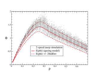
(b)

Figure 7: Comparison between the fundamental diagram simulated with exclusion processes and the one obtained from the corresponding (approximate) queuing process. The size is $L=1000$, $\delta$ is set to zero to have a TASEP (a), while the parameters are set to $\mu_{a}=10\times\mu_{b}=10\times\gamma=100\times\delta$ on panel (b).

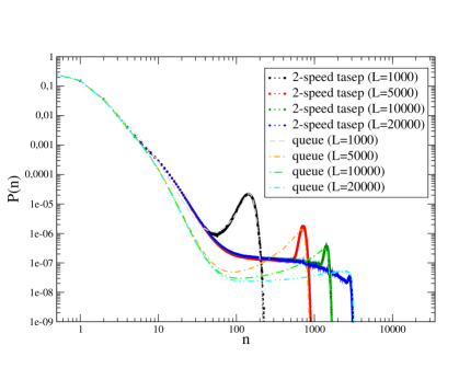
(a)

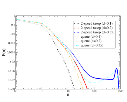
(b)

Figure 8: Comparison of particle cluster vs queue’s size distribution for set of parameters $\mu_{a}=10\mu_{b}=100$, $\gamma=10$ and $\delta=1$ for various sizes $L$ with fixed density $d=0.35$ (a) and various densities with fixed size $L=5000$ (b), the number of queues being $(1-d)L$.

From (34), we write down the cumulant generating function

$$h(s,t)=\log\Bigl{(}\pi_{0}\bigl{(}1+\frac{\mu_{b}e^{-\mu_{a}t}-\mu_{a}e^{-\mu_{b}t}}{\mu_{a}-\mu_{b}}\bigr{)}+\frac{(\mu_{a}-\lambda e^{-s})e^{-\mu_{b}t}+(\lambda e^{-s}-\mu_{b})e^{-\mu_{a}t}}{\mu_{a}-\mu_{b}}\ g(s)\Bigr{)}.$$

Therefore we get for the Hessian

$$\det\bigl{(}H(s^{\star},0)\bigr{)}=$$

$$\frac{1}{g^{2}}\left[\begin{matrix}\displaystyle gg^{\prime\prime}-g^{\prime 2}&g\bigl{(}\lambda e^{-s^{\star}}g+(1-\lambda e^{-s^{\star}})g^{\prime}\bigr{)}\\[5.69046pt] \displaystyle g\bigl{(}\lambda e^{-s^{\star}}g+(1-\lambda e^{-s^{\star}})g^{\prime}\bigr{)}&g\bigl{(}\mu_{a}\mu_{b}\pi_{0}+(\lambda(\mu_{a}+\mu_{b})e^{-s^{\star}}-\lambda^{2}-\mu_{a}\mu_{b})g\bigr{)}\end{matrix}\right],$$

where $s^{\star}$ is the point which satisfies

$$g^{\prime}(s^{\star})=-\rho.$$

from this we can compute the small (Gaussian) fluctuations of the FD. A comparison with the corresponding ABTASEP is displayed on Figure 7.

In addition to the fundamental diagram, under the canonical ensemble constraint, it is also interesting to determine the single queue distribution. This can be obtained from the partition function [16] in the large deviation framework as

$$p_{CE}(n,\mu) =\pi^{\lambda}(n,\mu)\frac{Z_{L-1}(N-n)}{Z_{L}(N)}$$

$$\simeq\pi^{\lambda}(n ,\mu)\exp\Bigl{[}L\bigl{(}h(s(d-x),0)-h(s(d),0)-\frac{d-x}{1-d-x}s(d-x)+\frac{d}{1-d}s(d)\bigr{)}\Bigr{]},$$

with $x\stackrel{{\scriptstyle\mbox{\tiny def}}}{{=}}n/(N+L)$ and the density constraint

$$\frac{\partial h}{\partial s}(s(d),0)=\frac{d}{1-d},$$

satisfied by $s(d)$. A comparison of this queueing formulation with the ABTASEP is given on Figure 8. In this case we impose an additional self-consistency condition on the parameter $\lambda_{a}$,

$$\lambda_{a}=\sum_{n=1}^{\infty}\pi_{n}^{a}\mu_{a},$$

which otherwise would be free. The correspondence between the cluster size distribution observed on the ABTASEP with the single queue distribution obtained from the generalized queueing process is rather accurate. In particular in both cases, a bump is observed in the distributions at the same location, for small size systems. It indicates that condensation is observed as a finite size phenomena. In the thermodynamic limit macroscopic jams are absent. In this respect it is different from the type of condensation analyzed in [16], which are obtained under some conditions on the service rate, as a large deviation principle but with different scaling (speed in the large deviation terminology) then $L$. Concerning the FD a larger discrepancy is observed between the ABTASEP process and its corresponding effective queueing process. The reason for this, which is not visible on the cluster distributions, is that the ratio of fast over slow particles for given size of cluster size does not coincide. We don’t know however which approximation between

• the simplified assumption on internal cluster structure

• the neglect of correlations between queues

in the effective model is responsible for that. These results indicate anyway that the steady state of the ABTASEP might be well accounted for by a little bit more refined joint cluster measure.

6 Conclusion and Perspectives

In this paper, motivated by questions raised in the context of traffic modelling, we have proposed a simple extension in the definition of the TASEP model to take into account acceleration and braking thereby offering the possibility to study the effect of asymmetry between the two mechanisms within a simple model. With two different speed levels a rich dynamics is already present. An effective mapping on a generalized zero-range process allows to interpret at least qualitatively the spontaneous jamming phenomena occurring in this model for some choice of parameters. In addition we develop a large deviation formalism to study the fundamental diagram associated to this family of queuing processes. Still the discrepancy between numerical simulation and estimation seen on Figures 8 and 7, may originate from the various approximations we make, concerning the detail structure of the jams and the correlations between queues which are neglected when using our large deviation estimation of the FD. This formalism could be possibly adapted to the situation where the joint measure of queues has not a product form.

In the family of models that we considered we found that condensation phenomena are associated to finite size effect on the ring geometry, and at least numerically the presence of a large macroscopic jam at large scale seems doomed to decay exponentially with no bump in the probability distribution, and this is consistent with the approximate mapping on zero-range process that we propose. Nevertheless the situations could change when the number of speed levels is increased, as shown in our previous work [15] on the subject, and we suspect that synchronized flow can take place in this limit of large number of speed level.

The situation where vehicles may enter or leave the system at very low rates so that the density may change adiabatically and allow to observed hysteresis effect deserves also more studies. In particular it would be interesting to find a relevant measure associated to trajectories in the FD, based for example on Brownian windings models proposed in [22], to quantify the hysteresis level in various regions of the FD.

Finally, the models considered here are limited to single lane traffic and could be easily generalized to multi-lane, using coupled exclusion processes like in [23].

Appendix A Complement to Section 4.2: constrained partition function and the dual Hessian

In this appendix we explain the role played by the dual Hessian in the Large deviation expression of the constrained partition functions. Assume that we have $n$ linear constraints, written as

$$Cy=V,$$

where $C$ is $n\times d$ matrix, each line $C_{i}$ corresponds to constraints $i$ and $V$ is a $n$-dimensional vector and that we want to estimate the constrained partition function $Z_{L}[V]$. To obtain the small fluctuations we approximate first $\cal F$ in (21) at second order with respect to some reference point $y^{*}$

$${\cal F}(y)={\cal F}(y^{*})+(y-y^{*})^{T}\cdot\bigtriangledown{\cal F}(y^{*})+(y-y^{*})^{T}\bigtriangledown^{2}{\cal F}(y^{*})(y-y^{*})+o\bigl{(}\|y-y^{*}\|^{2}\bigr{)},$$

so that $y$ considered as a $d$-dimensional vector is integrated over ${\mathbb{R}}^{d}$. $y^{*}$ is chosen such that

$$y^{*}(\Lambda)=\operatorname*{argmin}_{y}\ \Bigl{[}{\cal F}[y]-\Lambda^{T}Cy\Bigr{]},$$

matches the constraints with the proper Lagrange multipliers $\Lambda$. Since in absence of constraints $Z_{L}[V]$, as it stands in (20) is normalized to $1$, so at this order of approximation the partition function reads

$$Z_{L}[V]=L^{d/2}\sqrt{\frac{\det H}{(2\pi)^{d}}}\int d^{d}y\ e^{-L\bigr{(}{\cal F}(y^{*})+(y-y^{*})^{T}\cdot\bigtriangledown{\cal F}(y^{*})+\frac{1}{2}(y-y^{*})^{T}H(y-y^{*})\bigr{)}}$$

$$\times\prod_{i=1}^{n}\delta(V_{i}-\sum_{j=1}^{d}C_{ij}y_{j}),$$

with

$$H=\bigtriangledown^{2}{\cal F}(y^{*}),$$

the Hessian taken at $y=y^{*}$. The dual Hessian is associated to the dual free energy ${\cal F}^{\star}$,

$${\cal F}^{\star}[\Lambda]={\cal F}[y^{*}(\Lambda)]-\Lambda^{T}Cy.$$

Using relations associated to the stationarity of $y^{*}$, it reads

$$H^{\star}=C^{T}H^{-1}C.$$

Due to the specific form (22) of ${\cal F}$, the Hessian turns out to be the covariance matrix between the various quantities $V_{i}$, as given in (28). A convenient way to express the constraints is to write

$$\prod_{i=1}^{n}\delta(V_{i}-\sum_{j=1}^{d}C_{ij}y_{j})=\lim_{\alpha\to 0}\frac{1}{(2\pi\alpha)^{n/2}}e^{-\frac{1}{2\alpha}\|V-Cy\|^{2}},$$

so that a Gaussian integration over $y$ can be performed and since

$$\|V-Cy\|^{2}=\|C(y-y^{*}\|^{2},$$

we simply get

$$Z_{L}[V]=e^{-L{\cal F}(y^{*})}\lim_{\alpha\to 0}\sqrt{\frac{\det H}{(2\pi\alpha)^{n}\det H_{\alpha}}}e^{\frac{L}{2}V_{\alpha}^{T}H_{\alpha}^{-1}V_{\alpha}}$$

with

$$H_{\alpha} \stackrel{{\scriptstyle\mbox{\tiny def}}}{{=}}H+\frac{C^{T}C}{L\alpha}$$

$$V_{\alpha} \stackrel{{\scriptstyle\mbox{\tiny def}}}{{=}}\bigtriangledown{\cal F}(y^{*}).$$

Let $P$ be the orthonormal projection on the subspace spanned by the set of constraint vectors $C_{k}$ an $\bar{P}\stackrel{{\scriptstyle\mbox{\tiny def}}}{{=}}1-P$, such that

$$C=CP\qquad\text{and}\qquad P\ C^{T}=C^{T}.$$

We have

$$\det(H_{\alpha}) =\det(H)\det\bigl{(}1+\frac{C^{T}C}{L\alpha}H^{-1}\bigr{)}$$

$$=\det(H)\det\bigl{(}P(1+\frac{C^{T}C}{L\alpha}H^{-1})P+P\frac{C^{T}C}{L\alpha}H^{-1}\bar{P}+\bar{P}\bar{P}\bigr{)}$$

$$=\det(H)\det_{P}\bigl{(}1+\frac{C^{T}C}{L\alpha}H^{-1}\bigr{)}$$

$$=\det(H)\Bigl{(}\frac{1}{(L\alpha)^{n}}\det(H^{\star})+o\bigl{(}\frac{1}{\alpha^{n}}\bigr{)}\Bigr{)}$$

where $\det_{P}$ corresponds to the block determinant associated to the subspace of constraints, and

$$H^{\star}=C^{T}H^{-1}C$$

is the dual Hessian defined in (28). Concerning $V_{\alpha}$, since $y^{*}$ is a stationary point at least w.r.t. fluctuations orthogonal to the constraints, so we have

$$\bar{P}V_{\alpha}=0.$$

Since

$$H_{\alpha}^{-1} =H^{-1}\bigl{(}1+\frac{C^{T}C}{L\alpha}H^{-1}\bigr{)}^{-1}$$

$$=H^{-1}\bigl{(}PL\alpha H(C^{T}C)^{-1}P-P\bar{P}+\bar{P}\bar{P}\bigr{)}+o(\alpha),$$

as a result

$$\lim_{\alpha\to 0}\ V_{\alpha}^{T}H_{\alpha}^{-1}=0.$$

So finally the Gaussian estimate of the partition function reads

$$Z_{L}[V]=\frac{L^{n/2}}{\sqrt{(2\pi)^{n}\det(H^{\star})}}e^{-L{\cal F}(y^{*})}$$

which yield in particular the expressions (26,27) up to a factor $L^{n}$ caused by a different convention in the constraint definition.

Appendix B Complement to Section 5: steady state of the queueing process

From the master equations, taken at steady-state, we get the recurrence for $n\geq 2$

$$\lambda\bigl{(}\pi_{n-1}^{a}-\pi_{n}^{a}\bigr{)}+\bigl{(}\mu_{a}\pi_{n+1}^{a}+\mu_{b}\pi_{n+1}^{b}\bigr{)}p_{n}-\mu_{a}\pi_{n}^{a}+\gamma\pi_{n}^{b}=0,$$

$$\lambda\bigl{(}\pi_{n-1}^{b}-\pi_{n}^{b}\bigr{)}+\bigl{(}\mu_{a}\pi_{n+1}^{a}+\mu_{b}\pi_{n+1}^{b}\bigr{)}\bar{p}_{n}-\mu_{b}\pi_{n}^{b}-\gamma\pi_{n}^{b}=0.$$

For $n=1$, it reads

$$\lambda_{a}\pi_{0}-\lambda\pi_{1}^{a}+\bigl{(}\mu_{a}\pi_{2}^{a}+\mu_{b}\pi_{2}^{b}\bigr{)}p_{1}-\mu_{a}\pi_{1}^{a}+\gamma\pi_{1}^{b}=0,$$

$$\lambda_{b}\pi_{0}-\lambda\pi_{1}^{b}+\bigl{(}\mu_{a}\pi_{2}^{a}+\mu_{b}\pi_{2}^{b}\bigr{)}\bar{p}_{1}-\mu_{b}\pi_{1}^{b}-\gamma\pi_{1}^{b}=0.$$

The sum of the two equation gives that the quantity $\lambda\pi_{n}-\bigl{(}\mu_{a}\pi_{n+1}^{a}+\mu_{b}\pi_{n+1}^{b}\bigr{)}$ is a constant independent of $n$ which has to vanish, leading to the partial balance relation

$$\lambda\pi_{n}=\mu_{a}\pi_{n+1}^{a}+\mu_{b}\pi_{n+1}^{b},\qquad\forall n\geq 0.$$ (35)

Using this gives the relations,

$$\bigl{(}\mu_{a}+\lambda\bar{p}_{n+1}\bigr{)}\pi_{n+1}^{a}-(\gamma+\lambda p_{n+1})\pi_{n+1}^{b} =\lambda\pi_{n}^{a}$$ (36)

$$-\lambda\bar{p}_{n+1}\pi_{n+1}^{a}+(\gamma+\mu_{b}+\lambda p_{n+1})\pi_{n+1}^{b} =\lambda\pi_{n}^{b}.$$ (37)

The recurrence is then inverted to yield (31).

Recurrence (36,37) are then conveniently used to obtain the following relations among the generating functions,

$$\lambda_{a}g_{a}(rz)+\lambda_{a}g_{b}(rz) =(\mu_{a}+\lambda-\lambda z)g_{a}(z)-\gamma g_{b}(z)-\lambda_{a}\pi_{0}z$$

$$\lambda_{a}g_{a}(rz)+\lambda_{a}g_{b}(rz) =\lambda g_{a}(z)-(\gamma+\mu_{b}-\lambda z)g_{b}(z)+\lambda_{b}\pi_{0}z.$$

It follows that

$$g_{b}(z)=\frac{\lambda z}{\mu_{b}-\lambda z}\pi_{0}+\frac{\lambda z-\mu_{a}}{\mu_{b}-\lambda z}g_{a}(z),$$

also related to (35), which rewrites

$$g_{a}(z)=\frac{\mu_{b}}{\mu_{a}-\mu_{b}}\pi_{0}+\frac{\lambda z-\mu_{b}}{\mu_{a}-\mu_{b}}g(z),\qquad\text{and}\qquad g_{b}(z)=\frac{\mu_{a}}{\mu_{b}-\mu_{a}}\pi_{0}+\frac{\lambda z-\mu_{a}}{\mu_{b}-\mu_{a}}g(z).$$

So finally $g(z)$ satisfies the functional equation given in proposition 5.2. The solution is constructed as follows. Consider the infinite product

$$G(z)\stackrel{{\scriptstyle\mbox{\tiny def}}}{{=}}\prod_{n=0}^{\infty}\bigl{(}1-r^{n}\frac{z}{z^{+}}\bigr{)}\bigl{(}1-r^{n}\frac{z}{z^{-}}\bigr{)}.$$

We have

$$G(rz)=\frac{z^{-}z^{+}}{(z-z^{-})(z-z^{+})}G(z),$$ (38)

so a solution of the form

$$g(z)=\frac{C(z)}{G(z)}$$

has to verify

$$C(z)+\frac{u}{z^{+}z^{-}}C(rz)=\frac{w-vz}{(z-z^{-})(z-z^{+})}G(z).$$

Equivalently, for any $n\geq 0$ this rewrites

$$\bigl{(}-\frac{u}{z^{+}z^{-}}\bigr{)}^{n}C(r^{n}z)-\bigl{(}-\frac{u}{z^{+}z^{-}}\bigr{)}^{n+1}C(r^{n+1}z) =\bigl{(}-\frac{u}{z^{+}z^{-}}\bigr{)}^{n}\frac{w-vzr^{n}}{(zr^{n}-z^{-})(zr^{n}-z^{+})}G(r^{n}z)$$

$$=(-u)^{n}\frac{w-vzr^{n}}{\prod_{k=0}^{n}(zr^{k}-z^{-})(zr^{k}-z^{+})}G(z),$$

after using relation (38). Taking the sum leads to the solution (33), owing to

$$\lim_{n\to\infty}\bigr{(}-\frac{u}{z^{+}z^{-}}\bigl{)}^{n}C(r^{n}z)=0,$$

which can be checked afterwards.

Acknowledgments

We thank Guy Fayolle for useful discussions. This work was supported by the French National Research Agency (ANR) grant No ANR-08-SYSC-017.

References

- [1] M. Schreckenberg, A. Schadschneider, K. Nagel, and N. Ito. Discrete stochastic models for traffic flow. Phys. Rev., E51:2339, 1995.
- [2] B.S. Kerner. The Physics of Traffic. Springer Verlag, 2005.
- [3] M. Schönhof and D. Helbing. Criticism of three-phase traffic theory. Transportation Research, 43:784–797, 2009.
- [4] K. Nagel and M. Schreckenberg. A cellular automaton model for freeway traffic. J. Phys. I,2, pages 2221–2229, 1992.
- [5] R. Barlović, L. Santen, A. Schadschneider, and M. Schreckenberg. Metastable states in cellular automata for traffic flow. Eur. Phys. J., B5:793, 1998.
- [6] M. Blank. Hysteresis phenomenon in deterministic traffic flows. Journal of Statistical Physics, 120:627–658, 2005.
- [7] Y. Sugiyama et al. Traffic jams without bottlenecks: experimental evidence for the physical mechanism of the formation of a jam. New Journal of Physics, 10:1–7, 2008.
- [8] T. M. Liggett. Interacting Particle Systems. Springer, Berlin, 2005.
- [9] F. Spitzer. Interaction of Markov processes. Adv. Math., 5:246, 1970.
- [10] C. Appert and L. Santen. Boundary induced phase transitions in driven lattice gases with meta-stable states. PRL, 86:2498, 2001.
- [11] L. Cantini. Algebraic Bethe Ansatz for the two species ASEP with different hopping rates. J. Phys. A: Math. Theor., 41:095001, 2008.
- [12] V. Karimipour. A multi-species asep and its relation to traffic flow. Phys. Rev., E59:205, 1999.
- [13] B. Derrida, M. R. Evans, V. Hakim, and V. Pasquier. Exact solution for 1d asymmetric exclusion model using a matrix formulation. J. Phys. A: Math. Gen., 26:1493–1517, 1993.
- [14] M. Samsonov, C. Furtlehner, and J.M. Lasgouttes. Exactly solvable stochastic processes for traffic modelling. Technical Report 7278, INRIA, 2010.
- [15] C. Furtlehner and J.M. Lasgouttes. A queueing theory approach for a multi-speed exclusion process. In Traffic and Granular Flow ’ 07, pages 129–138, 2007.
- [16] M. R. Evans, S. N. Majumdar, and R. K. P. Zia. Canonical analysis of condensation in factorized steady states. Journal of Statistical Physics, 123(2):357–390, 2006.
- [17] K. Nagel and M. Paczuski. Emergent traffic jams. Phys. Rev. E, 51(4):2909–2918, 1995.
- [18] C.M. Harris. Queues with state-dependant stochastic service rate. Operation Research, 15:117–130, 1967.
- [19] F. P. Kelly. Reversibility and stochastic networks. John Wiley & Sons Ltd., 1979. Wiley Series in Probability and Mathematical Statistics.
- [20] H. Touchette. The large deviation approach to statistical mechanics. Physics Reports, 478:1–69, 2009.
- [21] G. Fayolle and J.-M. Lasgouttes. Asymptotics and scalings for large closed product-form networks via the Central Limit Theorem. Markov Proc. Rel. Fields, 2(2):317–348, 1996.
- [22] G. Fayolle and C. Furtlehner. Dynamical windings of random walks and exclusion models. J. Stat. Phys., 114:229–260, 2004.
- [23] M.R. Evans, Y. Kafri, K.E.P. Sugden, and J. Tailleur. Phase diagram of two-lane driven diffusive systems. arXiv:1103.4677.